Abstract
The standard ΛCDM model, despite its agreement with observational data, still has some issues unaddressed, such as the problem of initial singularity. Solving that problem usually requires modifications of general relativity. However, there appeared the Hořava–Lifshitz (HL) theory of gravity, in which equations governing cosmological evolution include a new term scaling similarly as the dark radiation term in the Friedmann equations, enabling a bounce of the universe instead of initial singularity. This review describes past works on the stability of such a bounce in different formulations of HL theory, an initial detailed balance scenario, and further projectable versions containing higher than quadratic terms to the original action.
1. Introduction
Classical general relativity (GR), apart from its simple beauty and symmetry, has also been strongly confirmed in several experimental tests. However, it does not explain many issues such as dark matter or space-time singularities, including the initial one in cosmology and those inside black holes. In order to answer these issues, there have been many attempts to modify GR both at the classical and quantum level. Specifically, the quantisation of GR cosmology was supposed to resolve the initial singularity problem.
Attempts to quantise gravity could be divided into two categories. One category involved assuming the classical theory of gravity and quantising it in various manners, with the first attempts performed via the covariant quantum gravity. In that classical approach, one repeats the method that was successful in quantising electrodynamics, namely considering the path integral of the Hilbert–Einstein action and then calculating the perturbation of the metric around a background one. The obtained equations, unlike in electrodynamics, are non-renormalizable in higher energies. Canonical quantum gravity considers the ADM -decomposition of space-time and the quantisation of the constraints obtained from the Hamiltonian. Other attempts have included sophisticated theories such as string theory and loop quantum gravity. These theories manage to solve some problems (such as the cosmological singularity [1]), but they are difficult to phenomenologically test [2,3]. The author of the present paper and colleagues used a combination of coherent states and Weyl quantisation in order to resolve an initial singularity problem; however, at this moment, the obtained models are difficult to validate by observational data [4].
Although there is still no full theory of quantum gravity that has been developed, it is supposed to manifest beyond a characteristic energy scale for quantum gravity built in terms of the speed of light c, the gravitational constant G, and Planck’s constant ℏ. Therefore, there is the second research direction, which aims to construct a modified version of GR with an improved UV behaviour. General relativity, after many tests performed, seems to be consistent with all current observations. This makes it a very good IR limit of a potential quantum gravity model. Some proposals have been made for UV completions of general relativity in the past [5,6]. They have one thing in common, namely the existence of some cutoff energy scale beyond which quantum effects could be detected, specially for a cutoff energy in the range of TeV. The widely discussed recent proposal is Hořava gravity, which is a proposal of a UV complete theory of gravity. It seems to be renormalizable at high energies, which makes it a candidate for a quantum gravity model [7,8]. The action of this theory contains additional higher order spatial derivatives, and therefore, the theory loses the full diffeomorphism invariance, keeping the (1 + 3) foliation preserving diffeomorphism. Moreover, there is a UV fixed point in this gravity model where there is an anisotropic Lifshitz scaling between time and space. Therefore, the resulting theory is called Hořava–Lifshitz (HL) gravity.
Significant work has been carried out on this theory examining different aspects and properties [9,10,11,12,13,14,15,16,17,18,19,20,21,22]. Many studies were devoted to cosmological solutions [12,19,23], including quantum cosmological ones [1,24,25,26,27,28,29], braneworlds, and dark radiation [12,21]. Hořava–Lifshitz cosmology obtained a novel feature enabling the existence of bounce instead of the initial singularity predicted by classical GR. There has also been other research focused on finding specific solutions, including black holes and their properties, and many works devoted to phenomenological aspects both astrophysical and concerning dark matter.
A derivation of Hořava–Lifshitz cosmology [12,19,23] made via varying-action written Friedmann–Robertson–Walker space-time metrics resulted in equations analogous to the standard Friedmann ones. These equations contain a new term that scales similarly as dark radiation [12,19,21], i.e., ∼1/ (where a is a scale factor) and provides a negative contribution to energy density. This feature enables obtaining non-singular cosmological evolution, resolving the initial singularity problem [14,21,30]. Such a possibility not only results in avoiding the initial singularity but may have other consequences for potential histories of the universe, such as the scenario of contraction from an infinite size connected by a bounce to expansion to infinite size again or eternal cycles of a similar scenario.
Despite many promises made by this modified theory of gravity, it seems that it contains instabilities and pathologies in different formulations (see, e.g., [22,31,32,33]). The original Hořava formulation suffers from many problems: the existence of ghost instabilities and strong coupling at IR [10,34], the appearance of a term that violates parity [22], very large values and negative signs of the cosmological constant [35,36], and issues with power-counting renormalisation of the propagation of the scalar mode [13,37]. Some of these problems might be solved by performing an analytic continuation of the parameters of the theory [20].
In the original Hořava formulation, it is assumed via the so-called detailed balance condition that a potential part of the action is derived from the so-called superpotential, which limits the big number of its terms and corresponding independent couplings. Another imposed condition is the demand of projectability, used in a standard cosmology. It requires that lapse function N depends only on time . It might seem that this condition is too strict, but on the other hand, it seems that the non-projectable version of Hořava gravity results in a serious strong coupling problem ([34]) and does not possess a valid GR limit at IR. However, some authors [35,38] claim the opposite, proposing adding additional terms to the superpotential (not to the action, thus still keeping detailed balance or eventually softly breaking it) and relaxing projectability. Nonetheless, subsequent works demonstrated that it caused problems with the scalar mode power-counting renormalizability.
One of the simplest models with the detailed balance condition relaxed is the Sotiriou–Visser–Weinfurtner (SVW) generalisation [22]. This version of HL gravity assumes a gravitational action containing terms not only quadratic in curvature but also cubic, as was suggested already in [12,19]. This model still maintains the projectability condition. Generalised Friedmann equations obtained from varying such an action contain not only a dark radiation term ∼1/ but also terms scaling with the ∼1/ term. These new terms, although negligible at large values of a, become dominating at small ones and might modify or cancel bounce solutions. Specifically, as it has the opposite sign as the term, it may compensate for the dark radiation term at small scales and result in singular solutions. A similar scenario arrives in the HL gravity with the softly broken detailed balance condition and negative spatial curvature [39].
Nonetheless, the issue of the initial singularity still remains one of the key questions of early universe cosmology. The possibility that it might be avoided in a modified gravity and replaced by a bounce is a very promising feature. In this review, we are going to present the result of the research [14,15] performed via phase portrait techniques on the occurrence and stability of the bounce in the two simplest formulations of HL cosmology: the original one with the imposed detailed balance (DB) condition and the beyond detailed balance (BDB) formulation relaxing this condition. As additional terms in analogs of Friedman equations are proportional to the curvature parameter , only non-flat cosmologies with allow the existence of a bounce and the existence of non-singular solutions.
The paper [14] was our first attempt at analysing the possibilities of a cosmological bounce in the original formulation of the theory. The matter sector was described there in terms of a scalar field with a potential given by a quadratic power of that field. However, that work included only a simplified version of the theory with either a vanishing cosmological constant or an HL universe with a non-zero in the region of a small scale factor a.
A more general approach that is easier to fit with observational data is the hydrodynamical approach used in [15], where the matter sector is described in terms of the density and pressure p. In the latter work, it was assumed that w, providing the relation between density and pressure in the equation of state, is constant, which is at some level an idealisation and simplification. At the moment, we do not have the history of the HL universe constructed in a similar way as in the standard ΛCDM model, where we have phases and epochs containing different matter or radiation sectors. Therefore, as we still have a limited understanding on the physical aspects of the theory and its parameters, current research rather describes different analytical possibilities, not some exact physical solutions.
It is important to mention that currently, HL theory and its extensions are not ruled out observationally (although there are tight bounds on some parameters [40]); thus, further observational constraints could shed new light on different specific scenarios or on the whole model, providing a better justification for deeper theoretical research. Several papers have placed bounds on different regions of the Hořava–Lifshitz framework, for example, using cosmological data [16], binary pulsars [41,42], and in the context of dark energy [43]. This has also occurred [18] in the effective field theory formalism of the the extended version of Hořava theory [31].
In [44,45], we investigated the same two basic Hořava–Lifshitz scenarios described earlier in the Introduction as a background theory for further numerical calculations. These calculations were devoted to fit observational data to two analogs of the Friedmann equations that arise in the mentioned HL scenarios. We did not limit our considerations to a flat model but left the curvature density parameter as a free parameter. In those papers, we provided improved observational constraints based on the recent cosmological data set from the cosmic microwave background (Planck CMB) [46], expansion rates of elliptical and lenticular galaxies [47], JLA compilation (joint light-curve analysis) data for Type Ia supernovae (SneIa) [48], Baryon acoustic pscillations (BAO) [49,50,51], and priors on the Hubble parameter [52].
Consequently, this review, on the one hand, presents our analytical studies of an HL universe aimed towards the possible existence of Big Bounce. On the other hand, we discuss the analytically obtained conditions on HL cosmology parameters that lead to the bounce and its corresponding observational constraints arrived at in our mentioned papers [44,45].
This paper is organised as follows: we first give a brief overview of HL cosmology in both scenarios under consideration in Section 2. In Section 3, the possibility of bounce in both formulations is discussed. Section 4 contains a derivation and description of the phase portraits of the HL cosmology with the imposed condition of detailed balance, while in Section 5, this condition is released. Section 6 contains a summary of results on the possibility of a bounce in HL cosmology. In Section 7, we discuss the possibility of a bounce, taking into account observational constraints, and present the limitation of the underlying theory.
2. Hořava–Lifshitz Cosmology
The main obstacle in quantising gravity is that general relativity in its classical formulation is non-renormalisable. This might be visualised by expanding some quantity with respect to the gravitational constant [33] as follows:
Here, E is the energy of the system, denotes a numerical coefficient, and is the gravitational coupling constant. Therefore, and the expansion above diverges. Consequently, as demonstrated, general relativity is not perturbatively renormalisable in the high energy regimes.
There have been many studies pointing out that the ultraviolet behaviour of general relativity might be improved by including higher-order derivatives in the standard gravitational metric. The latter is the Einstein–Hilbert action:
where d4x denotes the volume element of space-time, g is its metric matrix’s determinant, and R is a scalar curvature. Including-higher order terms of the derivatives of the metric provides the following action:
The additional terms, containing different derivatives of R, , etc., change the graviton propagator from into [7,8]. The propagator part proportional to cancels the ultraviolet divergence. However, the resulting theory has time derivatives of and is therefore non-unitary. Moreover, it possesses a spin-2 ghost with a non-zero mass [33] and derived form for which action field equations are of the fourth order.
The novel idea of Hořava [7] was to construct a higher-order theory of gravity breaking the Lorentz invariance in the ultraviolet range. In his theory, only the spatial derivatives are of , which evaded the ghost. However, it is necessary that any theory of gravity should be consistent with all current experiments that have not detected any significant violation of Lorentz invariance. Thus, it is necessary to restore the Lorentz invariance in the infrared limit. In order to overcome this problem, Hořava proposed an anisotropic scaling of space and time at high-UV energies, which is known as Lifshitz scaling. In a 4-dimensional space-time, this scaling takes the form:
where , and z is a critical exponent. Lorentz invariance is restored when , but the power-counting renormalizability demands [33], so usually is assumed. Therefore, the resulting theory is called Hořava–Lifshitz (HL) gravity. Lorentz symmetry is here broken down to transformations , preserving the spatial diffeomorphisms unlike the full space-time diffeomorphism invariance of GR. Thus, such a theory acquires a symmetry, preserving a space-time foliation [7,33], where on each constant time hypersurface, there are allowed arbitrary changes of the spatial coordinates.
Preservation of a space-time foliation and anisotropic scaling between time and space and time introduces the ADM (1 + 3)decomposition of the space-time. The standard ADM metrics in a preferred foliation and with a signature are as follows:
The dynamics are now described in terms of the lapse function N, the shift vector , and the spatial metric (i, ). The most general action for such theory can be written as:
Here, g denotes the determinant of the spatial metric , is a dimensionless running coupling constant, is a potential term, and K is a trace of the extrinsic curvature of the spatial 3-dimensional hypersurface :
An overdot denotes a derivative with respect to the time coordinate t. The trace of is K. The potential is invariant only under three-dimensional diffeomorphisms [31] and depends only on the spatial metric and its (spatial) derivatives. Thus, it contains only operators constructed from the spatial metric and of dimension 4 and 6.
2.1. Detailed Balance
As the action (6) is very complicated, Hořava [7,32,35] proposed to impose an additional condition, the so-called detailed balance. It assumes that could be derived from a superpotential W [7,32,35]:
and
By carrying out an analytic continuation (e.g., [20]) of the two constant parameters and , we obtain the action for Hořava–Lifshitz gravity in the detailed balance condition [32], which reads as
where is the Cotton tensor:
denotes the totally antisymmetric tensor. The parameters , and arriving in the theory have mass dimensions of, respectively, , 0, and 1. The analytic continuation mentioned above reads as and , and it enables obtaining the positive values of the cosmological constant as predicted by current observational results in the low-energy regime.
It is expected that action (10) reduces to the Einstein–Hilbert one in the IR limit of the theory. This is possible if the speed of light c and gravitational constant G correspond to HL parameters as follows:
The coupling constant present in the action (10) is dimensionless. It runs with energy and flows to the three infrared (IR) fixed points ([7]): , , or . However, some of those values seem unphysical. In the region , ghost instabilities appear in the IR limit of the theory [53]. The attempt to solve this problem [20] resulted in instabilities re-emerging at the other energy region, in the UV. Thus, the most physically interesting case is the regime that allows for a possible flow towards GR, where . Region , on the other hand, is disconnected from and therefore cannot be included in realistic physical considerations.
In order to obtain a cosmological model, it is necessary to populate the universe with matter (and radiation). The simplest method would be to model the matter sector by assuming it is described by a scalar field with a quadratic potential . However, a more realistic approach is to apply a hydrodynamic approximation where matter is described by two quantities p and , which are, respectively, pressure and energy density and fulfil the continuity equation .
To derive equations of HL cosmology, one uses the projectability condition [7], with the spatial part of the metrics being the standard FLRW line element: , where denotes a maximally symmetric metric with constant curvature:
where values correspond, respectively, to closed, flat, and open universes. This background metric implies that
where denotes the Hubble parameter.
On this background, the gravitational action (10) takes the following form:
In order to obtain equations of motion on a cosmological background, one needs to vary the action (15) with respect to N and a. Only after that can the lapse be set to one, , and terms with density and pressure p are added. This procedure provides the analogs to the Friedmann equations for the projectable Hořava–Lifshitz cosmology with the imposed detailed-balance condition:
together with the continuity equation:
In the equations above, there are two signs before the terms with ; namely, the upper one corresponds to the case, while the lower one describes the analytic continuation providing a positive .
Some terms in the above equations which scale as are similar to the dark energy expressions; therefore, the parameters of energy density and pressure density are interpreted as dark energy parameters:
We require that Equations (16) and (17) coincide with the standard Friedmann equations. Thus, we can identify the following:
respectively, as well as and (which is an IR fixed point). We demand a real value of the speed of light, c; therefore, the cosmological constant has to be negative for and positive for . In order to obtain a positive cosmological constant , as suggested by observations, it is necessary to perform in (10) an analytic complex continuation of constant parameters and as follows and . On the level of equations for Hořava–Lifshitz cosmology, varying -parameter in the range results in the running of the speed of light but does not change the structure of Equations (16) and (17).
2.2. Beyond Detailed Balance
The gravitational action (10) contains terms up to quadratic in the curvature. However, a more general renormalizable theory could also contain cubic terms, and there is not an a priori reason to keep only quadratic terms ([12,19,33]). Thus, Sotiriou, Visser, and Weinfurtner ([32]) built a projectable theory as the original Hořava theory but without imposing the detailed balance condition in the action.
This formulation led to Friedmann equations with an additional term ∼1/, moreover with additional and uncoupled coefficients:
In order to coincide with the Friedmann equations in the IR limit and for large a, when terms proportional to and to become negligibly small, one has to set and . However, values of the constants and are, at this stage, arbitrary. In this way, we obtain the following equations:
We can observe new terms in the above analogs of Friedmann equations proportional to . They mimic stiff matter, such that (), which scales similarly to . These terms are negligibly small at large scales but may play a significant role at small values of a scale parameter, thus changing the dynamics of the universe around initial singularity or a bounce.
3. Existence of Bounce
Hořava–Lifshitz cosmological equations contain additional terms proportional to (DB) and to (BDB) that introduce the possibility of a cosmological bounce, namely, a scenario in which contraction of the universe stops and reverses to expansion (or in the opposite direction). In a DB scenario, from the form of Equation (16), it follows that it is possible that . When this condition is fulfilled at some moment of time, the realisation of the bounce is possible (but not necessary; for that, we also need . In the case [12], the bounce may happen in a non-empty Universe equipped with matter at the critical time , , when the critical energy density reaches the following value:
This value is determined by the values of couplings and .
Additionally, a continuity equation implies that at the bounce, . Therefore, when the condition is fulfilled, we also have a sufficient condition for the existence of a bounce . is only possible as a transition from a contracting to an expanding phase, but not the reverse. Moreover, there is another condition for a realisation bounce [30] that requires that and the energy density of regular matter scales less quickly than dark matter terms.
Near the bounce—for small values of the parameter a—the dominating terms in the Friedmann Equations (22) and (23) are the terms scaling as , while other terms become insignificant. Particularly, , , and scale as , where w is a constant parameter in the equation of state . Subsequently, if , the density term dominates over the curvature term ∼1/.
In the BDB scenario, bounce might happen at the critical density:
For a flat universe and positive cosmological constant, bounce is not positive, as the resulting critical density becomes negative.
4. Bounce Stability in the Detailed Balance Formulation
We are mainly interested in the possibility of the appearance of a bounce that could be given by dynamics of variables a and H. From Equation (22), we might determine and then insert its formula into (23). This way, we obtain two systems, with one containing the formula for density and its derivative via the continuity Equation (22) but still dependent on a and H. The second system is independent and consists of two equations describing the evolution of a and H.
Specifically, Equation (22) provides the following expression for :
This expression substituted in (23) results in
Adding the the definition of the Hubble parameter:
we have a two dimensional dynamical system.
The set of Equations (31) and (32) is difficult to solve analytically. However, we are interested not in detailed solutions but in the qualitative analysis. For this purpose, we use the method of the phase portraits, where we search for critical points and analyse their character. These points are locations where the derivatives of all the dynamic variables, in our case when the r.h.s. of (31) and (32), vanish. What we obtain are the only points where phase trajectories could start, end, or intersect. Moreover, they can also appear in infinity. In this case, a suitable coordinate transformation, the so-called Poincaré projection, is used to project the complete phase space onto a compact region. The nature of these points, both finite and infinite, is given by the properties of the Jacobian matrix of the linearised equations at those points. All that information provides a qualitative analysis of the dynamical system.
The method of finding critical points consists of setting all right-hand sides of dynamical equations to zero, thus finding points where the derivatives of dynamical variables vanish. In the case of two equations, (31) and (32), the corresponding solutions are the two following and in the phase-space :
These two points exist when the values of a obtained via the square root of the expression on the right-hand side of the above equations are real and nonnegative. Thus the point exists if if we assume a positive cosmological constant, therefore, only for . Point exists when and or and . Thus, we have two critical points existing if the equation of state parameter . Moreover, they are both finite, unless , when blows to infinity. As mentioned above, due to , both points represent a bouncing solution.
In order to complete the analysis, the stability properties of the critical points are needed (rather informally, a stable critical point is one where, given any small distance to and any initial condition within a radius around , the trajectory of the system shall not go further away from than . An unstable critical point is the point which is not stable). They are determined by the eigenvalues of the Jacobian A of the system (31) and (32). Eigenvalues of A with non-zero real parts indicate hyperbolic points. They include sources (unstable) with positive real parts, saddles for real parts of opposite signs, and sinks (stable) corresponding to negative real parts. Critical points at which all the eigenvalues have real parts different from zero are called hyperbolic. Among them, one can distinguish sources (unstable) with positive real parts, saddles with real parts of different signs, and sinks (stable) for negative real parts. If at least one eigenvalue has a real part equal to zero it is then called a non-hyperbolic critical point. For such points, it is not possible to obtain conclusive information about the stability from the Jacobian matrix and other tools; e.g., numerical simulation [54] should be then used.
In the case of (31) and (32), the eigenvalues of A at are both imaginary, and it is a center for all the values of the parameters. The character of is more complicated and depends on the values of , K and w. Thus, is a center when and , with a special subcase for that being so it becomes a linear center, therefore becoming a center with only one eigenvector. Otherwise, it becomes a saddle and is thus without a bouncing possibility.
To obtain a full picture of the dynamics of the universe, the information about critical points that occur at infinity is also necessary. For this purpose, the so-called Poincaré projection [55,56] is used. It projects the whole infinite phase space onto a compact region. Specifically, we introduce the new coordinates , which are written in polar coordinates : and . Moreover:
It is also necessary to rescale the time parameter t, which takes infinite values, by introducing the new time parameter T in a similar way, i.e. . In such coordinates, the phase space is now compactified to a sphere of radius one and its interior. Here, infinity corresponds to . We have to keep in mind that a scale factor a may take only nonnegative values, thus actually being a semi-sphere (there is some small difference in interpreting phase trajectories in the original infinite phase space and in the Poincaré projected phase space. In the latter, there could be regions in which the parameter increases, although the parameter is negative, whereas this behaviour is absent in the former. This is due to the fact that parameters are geometric objects without the same physical meaning as the scale factor a and the Hubble parameter H).
This procedure provides the dynamical equations in terms of r, , and their derivatives with respect to the new time T. At the surface of the sphere, if we limit , there are 3 solutions , , , written in polar coordinates . These critical points are now hyperbolic unless , resulting in and being, respectively, a repelling and an attracting node. For points, and are non-hyperbolic, and numerical simulations provide that they are saddles and also ends of a separatrice.
The numerical phase portraits are presented in Figure 1, which contains the deformed phase space scaled to fit on the compactified sphere. We observe that bounce scenarios are only possible when one of the critical points and exist and is a center. Then, we have closed orbits around them, and the Universe might go through eternal cycles of expansion and collapse, connected by a bounce of a finite size, expansion, etc. However, the point describes a less physical bouncing solution with a density . A more interesting case is when is a center, as the density is non-zero at that point. The special case of provides a third bounce scenario around the linear center located now at ∞. In this case, the universe begins in a static infinite state as , then contracts to a finite size and rebounces to a static infinite universe.
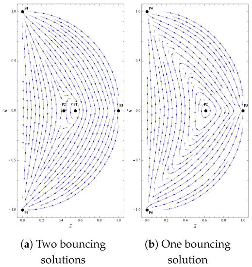
Figure 1.
Projected phase space of HL universe [15] in DB condition. Figure (a) is the case of and . Figure (b), , and .
5. Bounce Stability in the beyond Detailed Balance Formulation
In the Sotiriou, Visser, and Weinfurtner formulation, the generalised Friedmann Equations (26) and (27) contain additional terms ∼1/ and uncoupled coefficients.
Solving Equation (26) for provides:
Substituting this expression on into (27) and using the equation of state results in
As in the DB case, supplementing the above equation with the definition of the Hubble parameter provides the two-dimensional dynamical system.
Again, we search for critical points where and . These points fulfil and obtain the following condition:
This is a bicubic equation, which, in general, possesses quite complicated solutions but might be simplified in two special cases: namely when , describing the equation of state of the cosmological constant, and in the case of radiation described by . Outside of these two cases, critical points of the system (32) and (38) have the following coordinates: . Here, is a root of the cubic equation:
Such an equation might have zero, one, two, or three real solutions depending on the sign of its discriminant. Moreover, if they exist, they are either always stable or always unstable depending on the sign of . Their character depends on the values of , , , and . The most significant feature of oscillating (and bouncing) solutions in the SVW formulation is the existence of two centres with a saddle between them (three finite critical points) for some values of parameters. In a more realistic situation, that includes a dynamical change of state parameter, so it would be possible to go from one oscillating bouncing solution to another.
In order to study the stability properties of infinite critical points, one again has to perform the Poincarè transformation. This leads to similar results as in the detailed balance scenario. Points at infinity are transformed to the sphere . Two points at and at are, respectively, the repelling and attracting node, respectively. The point at is non-hyperbolic.
Figure 2 shows the example of the phase space of a system with three finite critical points. Here, points and are centres, and a point is a saddle.
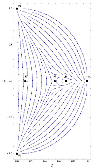
Figure 2.
Projected phase space of the HL universe in beyond detailed balance formulation with 3 critical points existing [15].
6. Discussion
This paper reviews the research performed on the occurrence and the properties of the cosmological bounce in different formulations of projectable versions of Hořava–Lifshitz gravity, with and without a detailed balance condition. The analogs of the Friedmann equations in both these models contain a term scaling as and similar to dark radiation. That additional term enables that the Hubble parameter might be at some moment of time. This is a necessary condition for the realisation of the bounce, while an additional condition makes it sufficient. In the Sotiriou, Visser, and Weinfurtner model, there is an additional term in the analogs of Friedmann equations. This term is of arbitrary sign, so it can enhance the possibility of a bounce or cancel it.
The biggest difference between the detailed balance theory and its breaking arrives for small values of a scale parameter a as the SVW gravity term plays role only for small values of a and becomes insignificant for bigger values. This difference is visible in the phase portraits of both theories and the number of potential bouncing solutions. In the original Hořava formulation, there exists one bouncing solution for all values of parameters, but it corresponds to a density of . For a non-zero , there might be a bouncing solution if and , but for other values of these parameters, a bounce is not possible.
The SVW HL cosmology is a bit more complicated as there are additional terms in the analogs of Friedmann equations. There exist bouncing solutions for some values of parameters of the theory; however, the range of parameters that lead only to singular solutions is wider than in the detailed balance scenario. One very interesting special case includes two centres with a saddle between them (corresponding to three finite critical points). If one takes into account the dynamical change of state parameter, which is a much more realistic scenario, it might be possible to go from one oscillating solution to another bouncing solution. The problem is that the existence of such solutions depends on the values of coupling constants and , and their physical interpretation still remains an open question.
Moreover, in both these formulations, bouncing non-singular solutions exist only in the case of a non-flat universe . In a DB scenario, from the form of Equations (33) and (34), it follows that for flat cosmologies with , the bounce happens at unless (stiff matter) or . In a zero-size universe, the metric becomes singular, and we cannot avoid an initial singularity. A similar situation happens in NDB. When we substitute into Equation (39), we then obtain Equation , providing the values of a for which the bounce happens. Again, unless or , the only solution is . Therefore, for most realistic values of w and , the only non-singular bouncing solutions arrive in non-flat cosmologies.
A specific subcase of described solutions is presented in [14] where, for the purpose of illustration, it was assumed that matter in the pre-bounce epoch is described by a scalar field with a quadratic potential. That paper describes the dynamics of a Hořava–Lifshitz universe in two simplified models: one with a vanishing cosmological constant and the other as an HL universe with a non-zero but in the region of a small scale factor a. These two limitations result from performing some simplifications in the equation of motion, which are valid only in the regime of a small a or in the case of .
However, even in those simplified settings, it was possible to answer the question of possible scenarios realising a bounce and whether it is generic for the theory or not. We have found stable solutions leading to a Big Crunch or starting at a Big Bounce, both staying within the regime of a small a. Compared to results with the standard cosmology [56], we observed that in the HL formulation, there were additional critical points allowing the existence of a bounce and enabling new possible families of trajectories.
7. Conclusions
The obtained cosmological results presented here are promising and suggest there is a possibility to replace the initial cosmological singularity of GR by finite bouncing solutions. However, one must also consider that there are many problems and contradicting statements in the different formulations and extensions of HL-type theories. Aside from that aspect, there are also observational bounds on the existence of the Hořava–Lifshitz gravity and the values of its constants and parameters.
At present, HL-type theories, including the original one and its extensions, are not yet ruled out by observational data. However, there now are tight bounds on some parameters of the theory [40] from the binary neutron star merger GW170817 [57]. Therefore, it is possible that further observational data might either rule out some specific scenarios or the whole model. It is also possible that some agreement with observations could provide a better justification for additional theoretical research, as it is still hoped that HL gravity could offer a promising cosmological scenario without an initial singularity and solve some shortcomings of classical GR, such as non-renormalizability and thus problems with quantisation.
There are several observational bounds on different regions of the Hořava–Lifshitz framework, e.g., using data from binary pulsars [41,42], using general cosmological data [16], and also bounds in the context of dark energy [43]. In the context of dark matter and dark energy, there are also bounds on general Lorentz violations [9,58]. There is also quite recent research performed in the effective field theory formalism [18] of the extension HL gravity [31]. However, this analysis is reduced to a flat background space-time, which limits the overall number of parameters.
As was presented above, bouncing non-singular solutions in two basic HL cosmological scenarios exist only in the case of a non-flat universe . Therefore, it is interesting to compare that condition to observational constraints on the curvature parameter. Particularly, in our papers [44,45], we have placed new bounds on the parameters of Hořava–Lifshitz cosmology in its projectable version with and without imposing detailed balance conditions. We found very interesting results on spatial curvature. Namely, in [44], the original HL model was well fitted with a non-zero spatial curvature with accuracy to more than , whereas when we relaxed the detailed balance condition, we again obtained a positive non-zero spatial curvature at 1 accuracy. In [45]. we used a larger and more updated dataset with additional high-energy sources such as quasars and gamma-ray bursts. We obtained that the HL universe both in the DB scenario and the NDB scenario is fitted with a negative curvature parameter at 1. On the other hand, similar calculations were made for ΛCDM model, such as in [59], where the negative curvature parameter was obtained from Planck data, weak galaxy lensing, and (supernovae and for the equation of state) local cosmic distance ladder measurements of the expansion rate.
As all those calculations included BAOs, therefore, there is a need for a further investigation of the curvature parameter, which could possibly finally exclude some of the HL models or zero-curvature ΛCDM models. Regardless, those results seem to be fascinating in view of future observations and also somehow demonstrate why an analysis limited to zero spatial curvature is somehow limited. Still, non-singular bouncing solutions in an HL universe appear only for non-zero spatial curvatures, so these two topics are related.
We have to take into account that most obtained bounds on the parameters of the HL cosmology are similar to those in the ΛCDM model. Of course, the ΛCDM model still has fewer parameters, and from this point of view should be preferred; it also fits the data well. However, one has to also bear in mind the theoretical aspects of Hořava gravity, which make it a good candidate for an ultraviolet complete theory of gravity. There are also several implications such as the possible resolution of the initial cosmological singularity, so there are still many reasons to keep investigating this model and its extensions.
Funding
This research received no external funding.
Conflicts of Interest
The author declares no conflict of interest.
Abbreviations
The following abbreviations are used in this manuscript:
| GR | General Relativity |
| SVW | Sotiriou-Visser-Weinfurtner |
| HL | Hořava-Lifshitz |
| ΛCDM | Lambda cold dark matter |
| ADM | Arnowitt, Deser and Misner |
| IR | Infrared |
| UV | Ultraviolet |
References
- Bojowald, M.; Date, G. Quantum Suppression of the Generic Chaotic Behavior Close to Cosmological Singularities. Phys. Rev. Lett. 2004, 92, 071302. [Google Scholar] [CrossRef]
- Quevedo, F. Is String Phenomenology an Oxymoron? 2016. Available online: http://xxx.lanl.gov/abs/1612.01569 (accessed on 23 March 2023).
- Girelli, F.; Hinterleitner, F.; Major, S. Loop Quantum Gravity Phenomenology: Linking Loops to Observational Physics. SIGMA Symmetry Integrability Geom. Methods Appl. 2012, 8, 098. [Google Scholar] [CrossRef]
- Bergeron, H.; Czuchry, E.; Gazeau, J.P.; Małkiewicz, P.; Piechocki, W. Singularity avoidance in a quantum model of the Mixmaster universe. Phys. Rev. D 2015, 92, 124018. [Google Scholar] [CrossRef]
- Arkani-Hamed, N.; Dimopoulos, S.; Dvali, G.R. The Hierarchy problem and new dimensions at a millimeter. Phys. Lett. B 1998, 429, 263–272. [Google Scholar] [CrossRef]
- Dvali, G. Black Holes and Large N Species Solution to the Hierarchy Problem. Fortsch. Phys. 2010, 58, 528–536. [Google Scholar] [CrossRef]
- Hořava, P. Quantum Gravity at a Lifshitz Point. Phys. Rev. D 2009, 79, 084008. [Google Scholar] [CrossRef]
- Hořava, P.; Melby-Thompson, C.M. General Covariance in Quantum Gravity at a Lifshitz Point. Phys. Rev. D 2010, 82, 064027. [Google Scholar] [CrossRef]
- Audren, B.; Blas, D.; Ivanov, M.M.; Lesgourgues, J.; Sibiryakov, S. Cosmological constraints on deviations from Lorentz invariance in gravity and dark matter. J. Cosmol. Astropart. Phys. 2015, 1503, 016. [Google Scholar] [CrossRef]
- Blas, D.; Pujolas, O.; Sibiryakov, S. On the Extra Mode and Inconsistency of Horava Gravity. J. High Energy Phys. 2009, 10, 029. [Google Scholar] [CrossRef]
- Blas, D.; Sanctuary, H. Gravitational Radiation in Hořava Gravity. Phys. Rev. D 2011, 84, 064004. [Google Scholar] [CrossRef]
- Calcagni, G. Cosmology of the Lifshitz universe. J. High Energy Phys. 2009, 9, 112. [Google Scholar] [CrossRef]
- Colombo, M.; Gümrükçüoğlu, A.E.; Sotiriou, T.P. Hořava gravity with mixed derivative terms: Power counting renormalizability with lower order dispersions. Phys. Rev. D 2015, 92, 064037. [Google Scholar] [CrossRef]
- Czuchry, E. The Phase portrait of a matter bounce in Hořava-Lifshitz cosmology. Class. Quant. Grav. 2011, 28, 085011. [Google Scholar] [CrossRef]
- Czuchry, E. Bounce scenarios in the Sotiriou-Visser-Weinfurtner generalization of the projectable Hořava-Lifshitz gravity. Class. Quant. Grav. 2011, 28, 125013. [Google Scholar] [CrossRef]
- Dutta, S.; Saridakis, E.N. Observational constraints on Hořava-Lifshitz cosmology. J. Cosmol. Astropart. Phys. 2010, 1001, 013. [Google Scholar] [CrossRef]
- Dutta, S.; Saridakis, E.N. Overall observational constraints on the running parameter λ of Hořava-Lifshitz gravity. J. Cosmol. Astropart. Phys. 2010, 1005, 013. [Google Scholar] [CrossRef]
- Frusciante, N.; Raveri, M.; Vernieri, D.; Hu, B.; Silvestri, A. Hořava Gravity in the Effective Field Theory formalism: From cosmology to observational constraints. Phys. Dark Univ. 2016, 13, 7–24. [Google Scholar] [CrossRef]
- Kiritsis, E.; Kofinas, G. Hořava-Lifshitz Cosmology. Nucl. Phys. B 2009, 821, 467–480. [Google Scholar] [CrossRef]
- Lü, H.; Mei, J.; Pope, C.N. Solutions to Hořava Gravity. Phys. Rev. Lett. 2009, 103, 091301. [Google Scholar] [CrossRef]
- Saridakis, E.N. Hořava-Lifshitz Dark Energy. Eur. Phys. J. C 2010, 67, 229–235. [Google Scholar] [CrossRef]
- Sotiriou, T.P.; Visser, M.; Weinfurtner, S. Quantum gravity without Lorentz invariance. J. High Energy Phys. 2009, 10, 033. [Google Scholar] [CrossRef]
- Mukohyama, S. Horava-Lifshitz Cosmology: A Review. Class. Quant. Grav. 2010, 27, 223101. [Google Scholar] [CrossRef]
- Bertolami, O.; Zarro, C.A.D. Hořava-Lifshitz quantum cosmology. Phys. Rev. D 2011, 84, 044042. [Google Scholar] [CrossRef]
- Pitelli, J.P.M.; Saa, A. Quantum Singularities in Horava-Lifshitz Cosmology. Phys. Rev. D 2012, 86, 063506. [Google Scholar] [CrossRef]
- Vakili, B.; Kord, V. Classical and quantum Hořava-Lifshitz cosmology in a minisuperspace perspective. Gen. Rel. Grav. 2013, 45, 1313–1331. [Google Scholar] [CrossRef]
- Oliveira-Neto, G.; Martins, L.G.; Monerat, G.A.; Corrêa Silva, E.V. De Broglie–Bohm interpretation of a Hořava–Lifshitz quantum cosmology model. Mod. Phys. Lett. A 2018, 33, 1850014. [Google Scholar] [CrossRef]
- Oliveira-Neto, G.; Martins, L.G.; Monerat, G.A.; Corrêa Silva, E.V. Quantum cosmology of a Hořava–Lifshitz model coupled to radiation. Int. J. Mod. Phys. D 2019, 28, 1950130. [Google Scholar] [CrossRef]
- Tavakoli, F.; Vakili, B.; Ardehali, H. Hořava-Lifshitz Scalar Field Cosmology: Classical and Quantum Viewpoints. Adv. High Energy Phys. 2021, 2021, 6617910. [Google Scholar] [CrossRef]
- Brandenberger, R. Matter bounce in Hořava-Lifshitz cosmology. Phys. Rev. D 2009, 80, 043516. [Google Scholar] [CrossRef]
- Blas, D.; Pujolas, O.; Sibiryakov, S. Consistent Extension of Hořava Gravity. Phys. Rev. Lett. 2010, 104, 181302. [Google Scholar] [CrossRef]
- Sotiriou, T.P. Hořava-Lifshitz gravity: A status report. J. Phys. Conf. Ser. 2011, 283, 012034. [Google Scholar] [CrossRef]
- Wang, A. Hořava gravity at a Lifshitz point: A progress report. Int. J. Mod. Phys. D 2017, 26, 1730014. [Google Scholar] [CrossRef]
- Charmousis, C.; Niz, G.; Padilla, A.; Saffin, P.M. Strong coupling in Hořava gravity. J. High Energy Phys. 2009, 8, 070. [Google Scholar] [CrossRef]
- Vernieri, D.; Sotiriou, T.P. Hořava-Lifshitz Gravity: Detailed Balance Revisited. Phys. Rev. D 2012, 85, 064003. [Google Scholar] [CrossRef]
- Appignani, C.; Casadio, R.; Shankaranarayanan, S. The Cosmological Constant and Horava-Lifshitz Gravity. J. Cosmol. Astropart. Phys. 2010, 4, 006. [Google Scholar] [CrossRef]
- Vernieri, D. On power-counting renormalizability of Hořava gravity with detailed balance. Phys. Rev. D 2015, 91, 124029. [Google Scholar] [CrossRef]
- Pospelov, M.; Shang, Y. On Lorentz violation in Horava-Lifshitz type theories. Phys. Rev. D 2012, 85, 105001. [Google Scholar] [CrossRef]
- Son, E.J.; Kim, W. Note on nonsingular cyclic universes in the deformed Horava-Lifshitz gravity. Mod. Phys. Lett. A 2011, 26, 719–725. [Google Scholar] [CrossRef]
- Emir Gumrukcuoglu, A.; Saravani, M.; Sotiriou, T.P. Hořava gravity after GW170817. Phys. Rev. D 2018, 97, 024032. [Google Scholar] [CrossRef]
- Yagi, K.; Blas, D.; Barausse, E.; Yunes, N. Constraints on Einstein-Æther theory and Hořava gravity from binary pulsar observations. Phys. Rev. D 2014, 89, 084067, Erratum in Phys. Rev. D 2014, 90, 069902; Erratum in Phys. Rev. D 2014, 90, 069901. [Google Scholar] [CrossRef]
- Yagi, K.; Blas, D.; Yunes, N.; Barausse, E. Strong Binary Pulsar Constraints on Lorentz Violation in Gravity. Phys. Rev. Lett. 2014, 112, 161101. [Google Scholar] [CrossRef]
- Park, M.i. A Test of Horava Gravity: The Dark Energy. J. Cosmol. Astropart. Phys. 2010, 1, 001. [Google Scholar] [CrossRef]
- Nilsson, N.A.; Czuchry, E. Hořava-Lifshitz cosmology in light of new data. Phys. Dark Univ. 2019, 23, 100253. [Google Scholar] [CrossRef]
- Czuchry, E.; Nilsson, N.A. On the energy flow of λ in Hořava-Lifshitz cosmology. arXiv 2023, arXiv:2304.09766. [Google Scholar] [CrossRef]
- Ade, P.A.R.; Aghanim, N.; Arnaud, M.; Ashdown, N.; Aumont, J.; Baccigalupi, C.; Banday, A.J.; Barreiro, R.B.; Bartlett, J.G.; Bartolo, N.; et al. Planck 2015 results. XIII. Cosmological parameters. Astron. Astrophys. 2016, 594, A13. [Google Scholar] [CrossRef]
- Moresco, M. Raising the bar: New constraints on the Hubble parameter with cosmic chronometers at z ∼ 2. Mon. Not. R. Astron. Soc. 2015, 450, L16–L20. [Google Scholar] [CrossRef]
- Betoule, M.; Kessler, R.; Guy, J.; Mosher, J.; Hardin, D.; Biswas, R.; Astier, A.; El-Hage, P.; Konig, M.; Kuhlmann, S.; et al. Improved cosmological constraints from a joint analysis of the SDSS-II and SNLS supernova samples. Astron. Astrophys. 2014, 568, A22. [Google Scholar] [CrossRef]
- Blake, C.; Brough, S.; Colless, M.; Contreras, C.; Couch, W.; Croom, S.; Croton, D.; Davis, T.M.; Drinkwater, M.J.; Forster, K.; et al. The WiggleZ Dark Energy Survey: Joint measurements of the expansion and growth history at z < 1. Mon. Not. Roy. Astron. Soc. 2012, 425, 405–414. [Google Scholar] [CrossRef]
- Alam, S.; Ata, M.; Bailey, S.; Beutler, F.; Bizyaev, D.; Blazek, J.A.; Bolton, A.S.; Brownstein, J.R.; Burden, A.; Chuang, C.H.; et al. The clustering of galaxies in the completed SDSS-III Baryon Oscillation Spectroscopic Survey: Cosmological analysis of the DR12 galaxy sample. Mon. Not. Roy. Astron. Soc. 2017, 470, 2617–2652. [Google Scholar] [CrossRef]
- Font-Ribera, A.; Kirkby, D.; Miralda-Escudé, J.; Ross, N.P.; Slosar, A.; Rich, J.; Aubourg, É.; Bailey, S.; Bhardwaj, V.; Bautista, J.; et al. Quasar-Lyman α Forest Cross-Correlation from BOSS DR11: Baryon Acoustic Oscillations. J. Cosmol. Astropart. Phys. 2014, 5, 027. [Google Scholar] [CrossRef]
- Bennett, C.L.; Larson, D.; Weiland, J.L.; Hinshaw, G. The 1% Concordance Hubble Constant. Astrophys. J. 2014, 794, 135. [Google Scholar] [CrossRef]
- Bogdanos, C.; Saridakis, E.N. Perturbative instabilities in Horava gravity. Class. Quant. Grav. 2010, 27, 075005. [Google Scholar] [CrossRef]
- Arrowsmith, D.K.; Place, C.M.; Place, C. An Introduction to Dynamical Systems; Cambridge University Press: Cambridge, UK, 1990. [Google Scholar]
- Felder, G.N.; Frolov, A.; Kofman, L. Warped geometry of brane worlds. Class. Quantum Gravity 2002, 19, 2983. [Google Scholar] [CrossRef]
- Felder, G.; Frolov, A.; Kofman, L.; Linde, A. Cosmology with negative potentials. Phys. Rev. D 2002, 66, 023507. [Google Scholar] [CrossRef]
- Abbott, B.P.; Abbott, R.; Abbott, T.D.; Acernese, F.; Ackley, K.; Adams, C.; Adams, T.; Addesso, P.; Adhikari, R.X.; Adya, V.B.; et al. Gravitational Waves and Gamma-rays from a Binary Neutron Star Merger: GW170817 and GRB 170817A. Astrophys. J. Lett. 2017, 848, L13. [Google Scholar] [CrossRef]
- Audren, B.; Blas, D.; Lesgourgues, J.; Sibiryakov, S. Cosmological constraints on Lorentz violating dark energy. J. Cosmol. Astropart. Phys. 2013, 8, 039. [Google Scholar] [CrossRef]
- Handley, W. Curvature tension: Evidence for a closed universe. Phys. Rev. D 2021, 103, L041301. [Google Scholar] [CrossRef]


Disclaimer/Publisher’s Note: The statements, opinions and data contained in all publications are solely those of the individual author(s) and contributor(s) and not of MDPI and/or the editor(s). MDPI and/or the editor(s) disclaim responsibility for any injury to people or property resulting from any ideas, methods, instructions or products referred to in the content. |
© 2023 by the author. Licensee MDPI, Basel, Switzerland. This article is an open access article distributed under the terms and conditions of the Creative Commons Attribution (CC BY) license (https://creativecommons.org/licenses/by/4.0/).