Abstract
In this paper, we study analytical approximate solutions for second-order homogeneous differential equations with the existence of only two turning points (but without poles) by using the uniform asymptotic approximation (UAA) method. To be more concrete, we consider the Pöschl–Teller (PT) potential, for which analytical solutions are known. Depending on the values of the parameters involved in the PT potential, we find that the upper bounds of the errors of the approximate solutions in general are ≲0.15∼10% for the first-order approximation of the UAA method. The approximations can be easily extended to high orders, for which the errors are expected to be much smaller. Such obtained analytical solutions can be used to study cosmological perturbations in the framework of quantum cosmology as well as quasi-normal modes of black holes.
Keywords:
loop quantum cosmology; cosmological perturbations; power spectrum; black holes; quasi-normal modes; gravitational waves PACS:
98.80.Cq; 98.80.Qc; 04.50.Kd; 04.60.Bc
1. Introduction
A century after the first claim by Einstein that general relativity (GR) needs to be quantized, the unification of quantum mechanics and GR still remains an open question despite enormous efforts [1,2]. Such a theory is necessary not only for conceptual reasons but also for the understanding of fundamental issues, such as the big bang and black hole singularities. Various theories have been proposed, and among them, string/M-Theory and loop quantum gravity (LQG) have been extensively investigated [3,4,5,6,7,8,9,10,11,12,13]. Differences between the two approaches are described in [14,15].
LQG was initially based on a canonical approach to quantum gravity (QG) introduced earlier by Dirac, Bergmann, Wheeler, and DeWitt [16,17]. However, instead of using metrics as the quantized objects [16,17], LQG is formulated in terms of densitized triads and connections and is a non-perturbative and background-independent quantization of GR [18,19]. The gravitational sector is described by the SU(2)-valued Ashtekar connection and its associated conjugate momentum, the densitized triad, from which one defines the holonomy of Ashtekar’s connection and the flux of the densitized triad. Then, one can construct the full kinematical Hilbert space in a rigorous and well-defined way [7,8,9,10,11,12,13]. An open question of LQG is its semiclassical limit: that is, are there solutions of LQG that closely approximate those of GR in the semiclassical limit?
Although the above question still remains open, concrete examples can be found in the context of loop quantum cosmology (LQC). (For recent reviews of LQC, see [20,21,22,23,24,25,26,27,28,29,30] and references therein.) Physical implications of LQC have also been studied using the effective descriptions of the quantum spacetimes derived from coherent states [31], whose validity has been verified numerically for various spacetimes [32,33,34,35,36,37], especially for states sharply peaked on classical trajectories at late times [38]. The effective dynamics provide a definitive answer to the resolution of the big bang singularity [39,40,41,42,43,44,45,46,47,48], which is replaced by a quantum bounce when the energy density of matter reaches a maximum value determined purely by the underlying quantum geometry.
To connect LQC with observations, cosmological perturbations in LQC have been also investigated intensively in the past decade, and a variety of different approaches to extend LQC to include cosmological perturbations have been developed. These include the dressed metric [49,50,51], hybrid [27,52,53,54], deformed algebra [55,56,57,58], and separate universe [59,60] approaches. For a brief review on each of these approaches, we refer readers to [29].
One of the major challenges in the study of cosmological perturbations in LQC is how to solve for the mode functions from the modified Mukhanov–Sasaki equation. So far, this has mainly been done numerically [20,21,22,23,24,25,26,27,28,29,30]. However, this is often required to be conducted with high-performance computational resources [61], which are not accessible to the general audience.
In the past decade, we have systematically developed the uniform asymptotic approximation (UAA) method initially proposed by Olver [62,63,64] and have applied it successfully to various circumstances [65,66,67,68,69,70,71,72,73,74,75,76,77,78,79,80,81,82,83,84,85] 1. In this paper, we continue work on this by considering the case in which the effective potential has only zero points but without singularities. To be more concrete, we consider the Pöschl–Teller (PT) potential, for which analytical solutions are known [86]. The consideration of this potential is also motivated by the studies of cosmological perturbations in dressed metric and hybrid approaches [87,88], in which it was shown explicitly that the potentials for the mode functions can be well-approximated by the PT potential with different choices of the PT parameters. In particular, in the dressed metric approach, the mode function satisfies the following equation [87]
in which serves as an effective potential. During the bouncing phase, it is given by
where is a constant introduced in [87], and and are, respectively, the Planck mass and time. This potential can be well-approximated by a PT potential
with
Here is the conformal time related to the cosmic time t by . On the other hand, in the hybrid approach, the effective potential is given by
which can be also modeled by the PT potential (3) but now with [88]
For more details, we refer readers to [87,88].
The rest of the paper is organized as follows: In Section 2, we provide a brief review of the UAA method with two turning points and show that the first-order approximate solution will be described by the parabolic cylinder functions. In Section 3, we construct the explicit approximate analytical solutions with the PT potential and find that the parameter space can be divided into three different cases: (A) , (B) , and (C) , where k and are real constants. After working out the error control function (cf. Appendix C) in each case, we are able to determine the parameter , which is introduced in the process of the UAA method in order to minimize the errors. Then, we show the upper bounds of errors of our approximate solutions with respect to the exact one given in Appendix B. In particular, in Case A), the upper bounds are ≲0.15%, while in Case B), they are no larger than . In Case C), the errors are also very small, except for the minimal points (cf. Figure 10), at which the approximate solutions deviate significantly from the analytical one. The causes of such large errors are not known and are still under our investigation. In each of these three cases, we also develop our numerical codes and find that the numerical solutions trace the exact one very well and that the upper bounds of errors are always less than in each of the three cases. The paper ends with Section 4, in which our main conclusions are summarized. There are also three Appendices Appendix A, Appendix B, and Appendix C, in which some mathematical formulas are presented.
2. The Uniform Asymptotic Approximation Method
Let us start with the following second-order differential equation
It should be noted that all second-order linear homogeneous ordinary differential equations (ODEs) can be written in the above form by properly choosing the variable y and . Instead of working with the above form, we introduce two functions and , so that the function takes the form [62]
where is a large positive dimensionless constant and serves as a bookmark, so we can expand as
After all the calculations are done, one can always set by simply absorbing the factor into . It should be noted that there exist cases in which the above expansion does not converge, and in these cases, we shall expand only to finite terms, say, , so that is well-approximated by the sum of these terms. On the other hand, the main reason to introduce two functions and , instead of only , is to minimize errors by properly choosing and .
In general, the function has singularities and/or zeros over the interval of our interest. We call the zeros and singularities of turning points and poles, respectively. The uniform asymptotic approximate (UAA) solutions of depend on the properties of around their poles and turning points [62,63,64]. The cases in which has both poles and turning points were studied in detail in [67,69,74], so in this paper, we shall focus ourselves on the cases where singularities are absent and only turning points exist. As to be shown below, the treatments of these cases will be different from the ones considered in [67,69,74]. In particular, in our previous studies, the function was uniquely determined by requiring that the error control function be finite and minimized at the poles, while in the current cases, no such poles exist. So to fix , other analyses of the error control function must be carried out.
2.1. The UAA Method
The UAA method includes three major steps: (i) the Liouville transformations, (ii) the minimization of the error control function, and (iii) the choice of the function , where is a new variable. In the following, we shall consider each of them separately.
2.1.1. The Liouville Transformations
The Liouville transformations consist of introducing a new variable , for which it is assumed that the inverse always exists and is thrice-differentiable. Without loss of generality, we also assume that is a monotonically increasing function (cf. Figure 1). Then, in terms of , which is defined by
Equation (7) takes the form
where
and
Figure 1.
The function vs. y, which is assumed to be an always increasing function of y.
It should be noted that Equations (7) and (11) are completely equivalent, and so far, no approximations have been taken. However, the advantage of the form of Equation (11) is that by properly choosing , the term can be much smaller than : that is,
so that the exact solution of Equation (7) can be well-approximated by the first-order solution of Equation (11) with . This immediately raises the question: how to choose so that condition (14) holds. To explain this in detail, let us move onto the next subsection.
2.1.2. Minimization of Errors
To minimize the errors, let us first introduce the error control function [62,63,64,67,69,74]
Then, introducing the free parameters and into the functions and , we have
where , with N being an integer. It is clear that for such chosen and , the error control function will also depend on and . To minimize the errors, one way is to minimize the error control function by properly choosing and so that
2.1.3. Choice of
On the other hand, the errors also depend on the choice of , which in turn sensitively depends on the properties of the functions and near their poles and turning points. In addition, it must be chosen so that the resulting equation of the first-order approximation (obtained by setting ) can be solved explicitly (in terms of known functions). Considering all the above, it has been found that can be chosen as [62,63,64,67,69,74]
in the cases with zero, one, and two turning points, respectively. Here for , and for .
In the rest of this paper, we shall consider only the cases with two turning points.
2.2. UAA Method for Two Turning Points
For the cases with two turning points, we can always write as
where and are the two turning points, and is a function of y, with , . In general, according to the properties of and , we can divide all the cases into three different subclasses:
- and are two distinct real roots of ;
- , a double real root of ;
- and are two complex roots of . Since is real, in this case, these two roots must be complex conjugate, .
To apply the UAA method to Equation (12), we assume that the following conditions are satisfied [67,69,74]:
- When far away from any of the two turning points, we require
- When near any of these two points, we requireprovided that the two turning points are far away from each other: that is, when .
- If the two turning points are close to each other, , then near these points, we require
It should be noted that when , the two turning points are far away, and each of them can be treated as an isolated single turning point [62,63]. In addition, without loss of generality, we assume that for or when and are real. When and are complex conjugate, we assume that (cf. Figure 2). Then, in this case, we adopt a method to treat all these three classes listed above together [64,67,69,74]. In particular, we choose as
so that is an increasing function of y (cf. Figure 1) and
When we integrate the above equation, without loss of generality, we shall choose the integration constants so that
Then, we find that
with
where corresponds to cases in which the two turning points and are both real, and corresponds to cases in which the two turning points and are complex conjugate. When and are complex conjugate, the integration of Equation (27) is along the imaginary axis [64]. When the two real roots are equal, we have .
Figure 2.
The function defined by Equation (39) for different choices of k and . In particular, the dotted black line denotes the case , and the solid blue line denotes the case , while the dash-dotted red line denotes the case .
To proceed further, let us first derive the relation between and y by first integrating the right-hand side of Equation (24). To this goal, it is found to be easier to distinguish the case in which and are real from the one in which they are complex conjugate.
2.2.1. When Are Real
2.2.2. When Are Complex Conjugate
Now let us turn to consider the case when and are complex. For this case, is always negative, ; thus, from Equation (10), we find [64]
2.2.3. The First-Order Approximate Solutions
With the choice of Equation (23), we find that Equation (12) reduces to
where we assume that , with being a real and positive constant, which can be arbitrarily large .
Neglecting the term, we find that the approximate solutions can be expressed in terms of the parabolic cylinder functions [64], and are given by
from which we have
where and are two integration constants, and and are the errors of the corresponding approximate solutions, whose upper bounds are given by Equations (A1) and (A2) in Appendix A.
3. UAA Solutions with the Pöschl–Teller Potential
To study the case in which only turning points exist, in this paper, we consider the second-order differential Equation (7) with a Pöschl–Teller (PT) potential [87,88]
as in this case exact solutions exist, where k is the comoving wavenumber, and is a real and positive constant. The two parameters and determine the height and the spread of the PT potential, respectively. Under the rescaling , the parameter can be absorbed into the wavenumber k and by redefining . As a result, there is no loss of generality to set from now on. Then, the exact solutions in this case exist and are presented in Appendix B.
On the other hand, to apply the UAA method to this case and to minimize the errors of the analytic approximate solutions, we tentatively choose q as
where is a free parameter to be determined below by minimizing the error control function (15) with the choice of given by Equation (23). Then, we have
where . In this paper, without loss of generality, we shall choose so that is always real: that is
Thus, from we find that the two roots are given by
It is clear that, depending on the relative magnitudes of and k as well as the choices of , two turning points can be either complex or real. In Figure 2, we plot out the three different cases, , , and , from which it can be seen clearly that the two turning points are real and different for , real and equal for , and complex conjugate for . Then, from Equations (38) and (39), we find that
for ,
for and , and
for and . In the following, let us consider the three cases: (a) , (b) , and (c) separately.
3.1.
In this case, we have is always negative, , so that the two turning points of are complex conjugate and are given by
As discussed in the last section, now , for which Equation (32) can be cast in the form
where . Note that in writing down the above equation, we replaced U with W. In addition, the new variable is related to y via
from which we find that is given explicitly by
Moreover, in the case of the PT potential, the integration of Equation (47) can be carried out explicitly, giving
where denotes the sign of y, with , and is the Appell hypergeometric function. Ignoring the term in Equation (46), we find the general solution
where W denotes the Weber parabolic cylinder function [89], and and are two integration parameters that generally depend on the comoving wavenumber k.
The validity of the analytic solution (50) depends on the criteria given by Equations (20)–(22), while its accuracy can be predicted by the error control function . In the current case, we find that of Equation (35) can be written as a combination of the three terms given by Equations (A10) 2, where
where A is given by Equation (A12). It should be noted that , , and given in Equation (51) all vanish when (for which we have and ); that is,
Further, as the PT potential is an even function, the error control function is antisymmetric about the origin: namely, . As a result, we will study its behavior only on the positive y axis, . With the help of Equation (47), the numeric value of the error control function at any point can be found from Equation (51). In particular, for , we find that
as (or ). Note that as , which can be seen clearly from Equation (47). Thus, to minimize the error control function for very large values of y, we must choose
In Figure 3, we plot the functions , , and together with the error control function defined by Equations (A10)–(A12) for , with being given by Equation (54). (Recall .) From these figures, it is clear that the conditions (20)–(22) are well-satisfied, and the error control function remains small all the time. In particular, it decreases as decreases.
Figure 3.
Plots of the quantities , , , and the error control function for , , and , for which we have .
In Figure 4, we plot the mode functions , , , and the relative difference defined by
where , denotes the mode function obtained by the UAA method given by Equation (50), is the numerical solution obtained by integrating Equation (7) directly with the same initial conditions, while is the exact solution given by Equation (A7). From these figures, we can see that the maximal errors occur in the region near , but the upper bound is no larger than at any given y, including the region near .
Figure 4.
Plots of the mode functions and their relative differences and for , and , for which we have .
It is interesting to note that this analytical approximate solution is only up to the first-order approximation of the UAA method. With higher-order approximations, the relative errors are even smaller.
To check our numerical solutions, in Figure 4 we also plot the relative differences between and , defined by
From these figures, it can be seen that is no larger than , and our numerical code is well-tested and justified.
It is also interesting to note that the mode functions are oscillating for , and these fine features are captured in all three mode functions, although there are some differences in the details. Again, as shown by their relative variations, these differences are very small. In addition, we also consider other choices of and k and find that they all have similar properties under the condition .
3.2.
In this case, depending on or , the function has different properties, as shown in Figure 2. Therefore, in the following subsections, let us consider them separately.
3.2.1.
When , the function is always non-positive for . Then from Equations (A10) and (51), we find that
as , but now we have . Thus, to have the error control function be finite at , now we must set
instead of the value given by Equation (54) for the case . In Figure 5, we plot the quantities , , , and the error control function for , , and , for which we have . From these figures, we can see clearly that the conditions (20)–(22) are well-satisfied, and the error control function remains small all the time. Then, the corresponding quantities , , , , and are plotted in Figure 6. From the curves of and , we can see that now the errors of the first-order UAA solution are , which are larger than those of the last subcase. This is mainly because of the fast oscillations of the solution in the region . Therefore, in order to obtain solutions with high precision, high-order approximations for this case are needed. However, we do like to note that our numerical solution still matches the exact one very well, as shown by the curve of , which is no larger than .
Figure 5.
Plots of the quantities , , , and the error control function for , , and , for which we have .
Figure 6.
Plots of the mode functions and and their relative differences , and for , , and .
3.2.2.
In this case, we find that
On the other hand, from Equations (36), (A10) and (A13), we find that
where . Note that in calculating the error control function near the turning point , we used the relation
so that the divergence of the second term of cancels exactly with that of . Equation (61) can be obtained directly from the relation for the case . Similarly, it can be shown that
It is clear that to minimize the errors, in the present case, must also be chosen to be
as given by Equation (58). In Figure 7, we plot the quantities , , , and the error control function for , , and , for which we have . It is clear that in this case, the two turning points are very close, and the conditions and are violated near these points. However, the condition holds near them. So, conditions (20)–(22) are also satisfied, and the error control function remains small all the time.
Figure 7.
Plots of the quantities , , , and the error control function for , , and , for which we have .
Then, the corresponding quantities , , , , and are plotted in Figure 8. From the curves of and , we can see that now the errors of the first-order UAA solution are . Similar to the last subcase, this is mainly because of the fast oscillations of the solution in the region . Therefore, in order to obtain high precision, high-order approximations for this case are needed, too. In addition, our numerical solution still matches well with the exact one, as shown by the curve of , which is no larger than .
Figure 8.
Plots of the mode functions and and their relative differences , and for , , and .
3.3.
In this case, two real turning points appear, given, respectively, by
Then, we find that Equations (59) and (60) still hold in the current case, while Equation (61) is replaced by
as , but now we have . Combining Equations (59), (60) and (65), we find that currently the proper choice of is still that given by , as in the last two subcases.
In Figure 9, we plot the quantities , , , and the error control function for , , and , for which we have . From this figure, we can see that the preconditions (20)–(22) are well-satisfied. Then, for the first-order approximation of the UAA method, the solution can be approximated by Equation (34), where is given by Equation (59), and are two integration constants, and and are the errors of the corresponding approximate solutions, whose upper bounds are given by Equations (A1) and (A2) in Appendix A.
Figure 9.
Plots of the quantities , , , and the error control function for , , and , for which we have .
In Figure 10a, we plot out our first-order approximate solution, while Figure 10b is used to compare the approximate solution with the exact one, so e plot both of them. In particular, the solid line represents the exact solution, while the red dotted line is the approximate solution. From this figure, it can be seen that except for the minimal points, the two solutions match well. However, at these extreme minimal points, they deviate significantly from each. The causes of such errors are not clear, and we hope to come back to this issue on another occasion.
Figure 10.
Plots of the mode functions (a) and (b) and their relative differences (d) , and (f) for , , and , for which we have .
Finally, similar to all other cases, our numerical solution still matches well with the exact one, as shown by the curve of , which is no larger than .
4. Conclusions
In this paper, we have applied the UAA method to the mode function with a PT potential, for which it satisfies the second-order differential equation
where k and are real constants. In this case, the exact solution is known and is given by Equation (A7). The implementation of the UAA method includes the introduction of an auxiliary function , which is taken as
where is a free parameter. Then, we carry out the integration of the error control function, defined by
where
Clearly, the error control function will depend on . After working out the details, we find that it is convenient to distinguish between three cases: A) , B) , and C) , where . In particular, in Case A), a proper choice of is , while in Cases B) and C), it is .
Once is fixed, the analytical approximate solutions are uniquely determined by the linear combination of the two parabolic cylinder functions , as shown by Equation (34). In particular, in Case A), the upper bounds of errors are ≲0.15%, as shown in Figure 4. In Case B), two subcases are considered: one with and the other with . In the first case, the upper bounds of errors are , while in the second case, they are ≲ 10%, as shown, respectively, in Figure 6 and Figure 8. In Case C), the approximate solutions also trace very well to the exact one, except for the minimal points, as shown in Figure 10. This might be caused by the fact that at these points, the mode function is almost zero, and very small non-zero values will cause significantly deviations. We are still working on this case and hope to come back to this point on another occasion.
As mentioned in the Introduction, the potentials of the mode functions in both dressed metric and hybrid approaches can be well-modeled by PT potentials. Therefore, the current analysis of the choice of the function and the minimization of the error control function shall shed great light on how to carry out similar analyses in order to obtain more accurate approximate solutions in these models. We have been working on it recently and wish to report our results soon on another occasion.
In addition, the differential equations for the quasi-normal modes of black holes usually also take the form of Equation (7) with potentials that have no singularities 3, but normally do have turning points [90,91]. For example, the effective potential for the axial perturbations of the Schwarzschild black hole is given by
where denotes the quasi-normal mode. Clearly, for , this potential also has no poles, but in general has two turning points. From [90,91], it can be seen that the properties of this potential are shared by many other cases, including those from modified theories of gravity. Thus, one can equally apply the analysis presented here to the studies of quasi-normal modes of black holes.
Author Contributions
All the authors have the equal contributions. All authors have read and agreed to the published version of the manuscript.
Funding
RP and AW were partially supported by the US Natural Science Foundation (NSF) under grant No. PHY2308845, and JJM and JS were supported through the Baylor Physics graduate program. BFL and TZ were supported in part by the National Key Research and Development Program of China under grant No. 2020YFC2201503; the National Natural Science Foundation of China under grant Nos. 11975203, 11675143, 12205254, 12275238, and 12005186; the Zhejiang Provincial Natural Science Foundation of China under grant Nos. LR21A050001 and LY20A050002; and the Fundamental Research Funds for the Provincial Universities of Zhejiang in China under grant No. RF-A2019015.
Data Availability Statement
No additional data are needed.
Acknowledgments
We thank the Special Issue Editor for his kind invitation and organization.
Conflicts of Interest
The authors declare no conflict of interest.
Appendix A. Upper Bounds of Errors
Appendix B. Exact Solutions with the Pöschl–Teller Potential
Let us consider the case with the Pöschl–Teller Potential given by
Then, introducing the two new variables x and via the relations
we find that Equation (7) with the above PT potential reads
where
Equation (A5) is the standard hypergeometric equation and has the general solution [87]
Here denotes the hypergeometric function, and and are two independent integration constants that are uniquely determined by the initial conditions.
Appendix C. Computing the Error Control Function
In this appendix, we collect some useful formulae for working out the error control function explicitly. Considering the particular form of the PT potential, it is easier to compute the error control function by using the new variable ; thus,
where denotes the sign of y. In terms of the new variable,
To calculate the error control function explicitly, let us consider the cases and separately.
Appendix C.1. g < 0
In this case, the error control function is defined by Equation (35), which can be written as
where
where
Appendix C.2. g > 0
Notes
| 1 | It should be noted that the first application of the UAA method to cosmological perturbations in GR was carried out by Habib et al. |
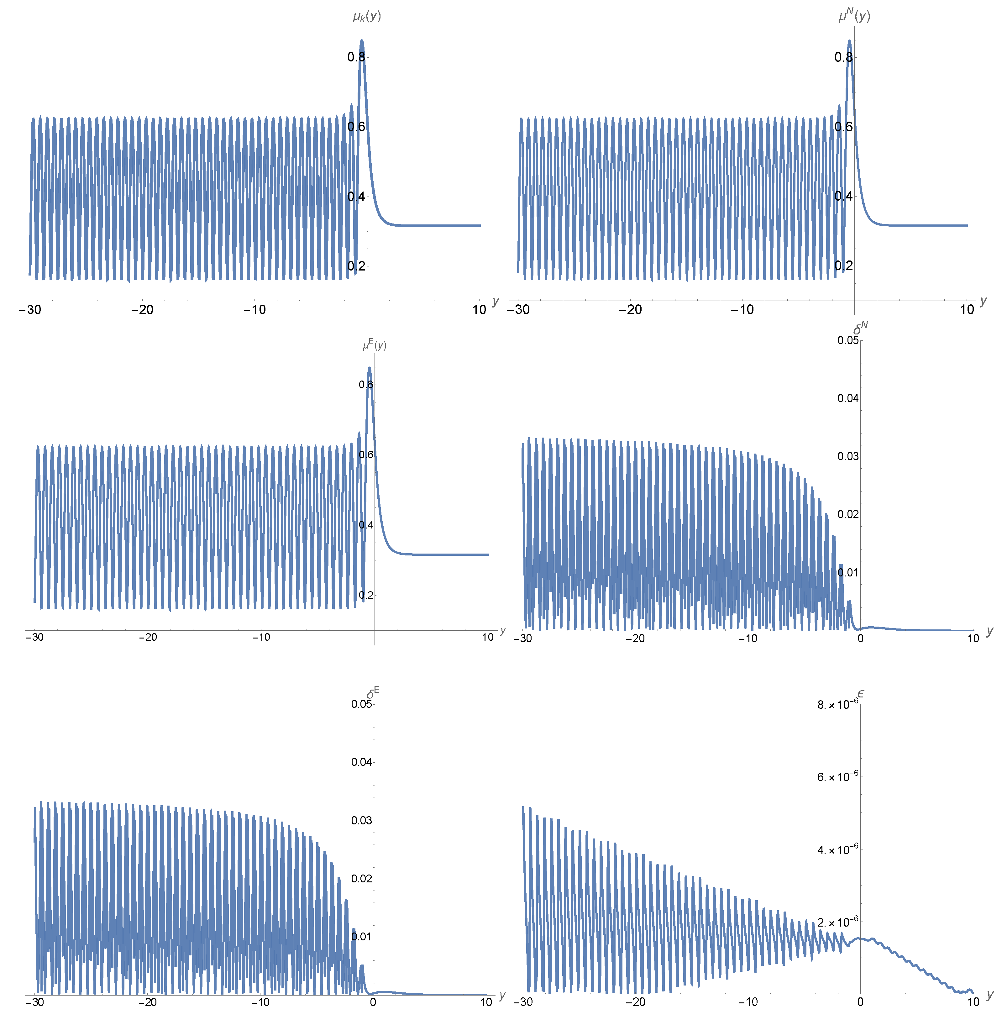
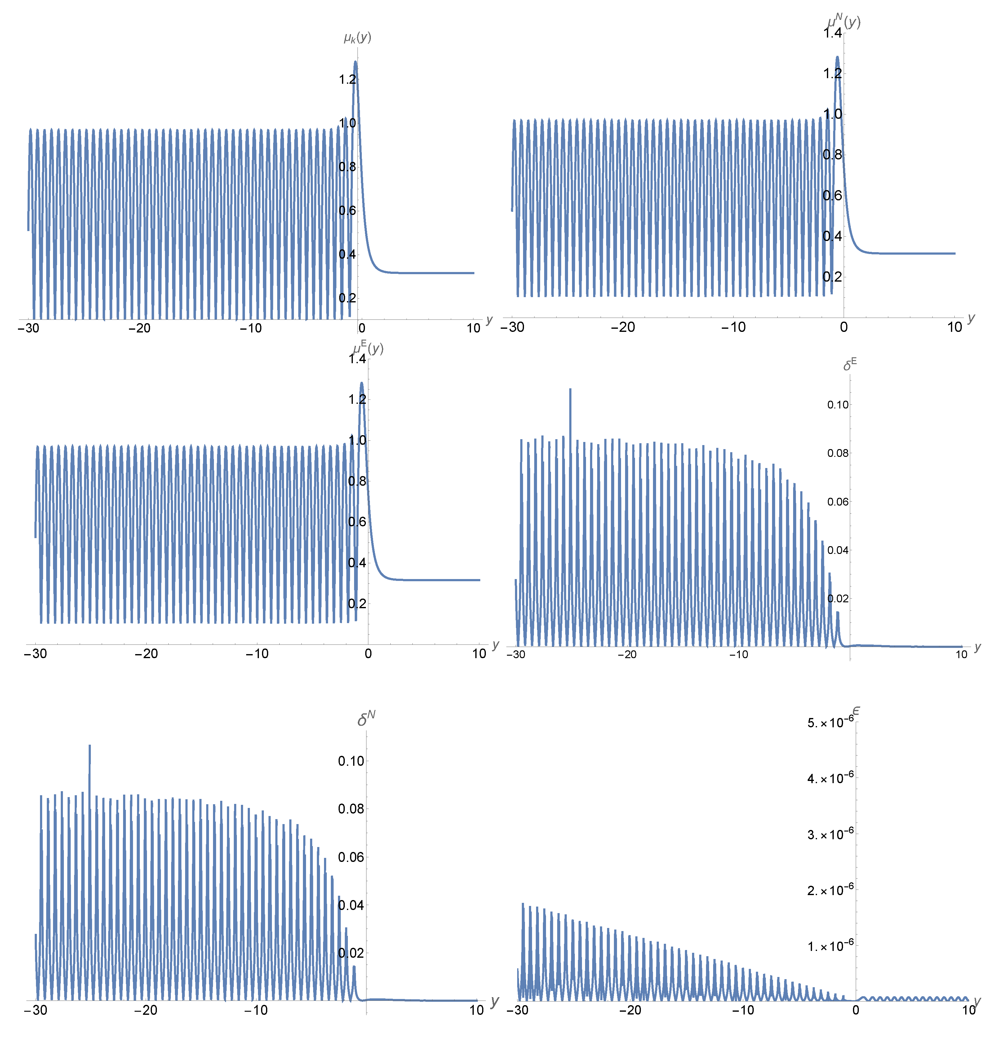
| 2 | In this case, the associated error control function is for any given , where [64]. In this paper, we choose , so the integrations will be carried out over the interval , corresponding to . Due to the symmetry of the equation, one can easily obtain the solutions for the region by simply replacing y by (or by )) |
| 3 | Recall the inner boundaries of black hole perturbations are the horizons, at which the potentials are usually finite and non-singular. |
| 4 | This corresponds to choosing the function introduced by Olver in [64] as , which satisfies the requirement as . For more details, see [64]. |
References
- Kiefer, C. Quantum Gravity, 3rd ed.; Oxford Science Publications, Oxford University Press: Oxford, UK, 2012. [Google Scholar]
- Hamber, H.W. Quantum Gravity, the Feynman Path Integral Approach; Springer: Berlin/Heidelberg, Germany, 2009. [Google Scholar]
- Green, M.B.; Schwarz, J.H.; Witten, E. Superstring Theory; Cambridge Monographs on Mathematical Physics; Cambridge University Press: Cambridge, UK, 1999; Volumes 1–2. [Google Scholar]
- Polchinski, J. String Theory; Cambridge University Press: Cambridge, UK, 2001; Volumes 1–2. [Google Scholar]
- Johson, C.V. D-Branes; Cambridge Monographs on Mathematical Physics; Cambridge University Press: Cambridge, UK, 2003. [Google Scholar]
- Becker, K.; Becker, M.; Schwarz, J.H. String Theory and M-Theory; Cambridge University Press: Cambridge, UK, 2007. [Google Scholar]
- Ashtekar, A.; Lewandowski, J. Background independent quantum gravity: A status report. Class. Quant. Grav. 2004, 21, R53. [Google Scholar] [CrossRef]
- Thiemann, T. Modern Canonical Quantum General Relativity; Cambridge Monographs on Mathematical Physics; Cambridge University Press: Cambridge, UK, 2007. [Google Scholar]
- Rovelli, C. Quantum Gravity; Cambridge University Press: Cambridge, UK, 2008. [Google Scholar]
- Bojowald, M. Canonical Gravity and Applications: Cosmology, Black Holes, and Quantum Gravity; Cambridge University Press: Cambridge, UK, 2011. [Google Scholar]
- Gambini, R.; Pullin, J. A First Course in Loop Quantum Gravity; Oxford University Press: Oxford, UK, 2011. [Google Scholar]
- Rovelli, C.; Vidotto, F. Covariant Loop Quantum Gravity; Cambridge University Press: Cambridge, UK, 2015. [Google Scholar]
- Ashtekar, A.; Pullin, J. Loop Quantum Gravity, the First 30 Years; World Scientific: Singapore, 2017. [Google Scholar]
- Thiemann, T. The LQG String—loop quantum gravity quantization of string theory: I. Flat target space. Class. Quamtum Grav. 2006, 23, 1923. [Google Scholar] [CrossRef]
- Helling, R.C.; Giuseppe, P. String quantization: Fock vs. LQG representations. arXiv 2004, arXiv:hep-th/0409182. [Google Scholar]
- Witt, B.S.D. Quantum Theory of Gravity. I. The Canonical Theory. Phys. Rev. 1967, 160, 1113. [Google Scholar]
- Wheeler, J.A. Relativity, Groups and Topology; Witt, C.M.D., Wheeler, J.A., Eds.; Benjamin: New York, NY, USA, 1968. [Google Scholar]
- Ashtekar, A. New variables for classical and quantum gravity. Phys. Rev. Lett. 1986, 57, 2244. [Google Scholar] [CrossRef] [PubMed]
- Ashtekar, A. New Hamiltonian formulation of general relativity. Phys. Rev. D 1987, 36, 1587. [Google Scholar] [CrossRef] [PubMed]
- Bojowald, M. Loop Quantum Cosmology. Living Rev. Relativ. 2008, 11, 4. [Google Scholar] [CrossRef]
- Bojowald, M. Quantum cosmology: A review. Rep. Prog. Phys. 2015, 78, 023901. [Google Scholar] [CrossRef]
- Ashtekar, A.; Singh, P. Loop Quantum Cosmology: A Status Report. Class. Quant. Grav. 2011, 28, 213001. [Google Scholar] [CrossRef]
- Ashtekar, A.; Barrau, A. Loop quantum cosmology: From pre-inflationary dynamics to observations. Class. Quant. Grav. 2015, 32, 234001. [Google Scholar] [CrossRef]
- Singh, P. Loop Quantum Cosmology. Int. J. Mod. Phys. D 2016, 25, 8. [Google Scholar]
- Agullo, I.; Singh, P. Loop Quantum Cosmology. In Loop Quantum Gravity: The First 30 Years; Ashtekar, A., Pullin, J., Eds.; World Scientific: Singapore, 2017. [Google Scholar]
- Wilson-Ewing, E. Testing loop quantum cosmology. Comptes Rendus Phys. 2017, 18, 207. [Google Scholar] [CrossRef]
- Navascués, B.E.; Marugán, G.A.M. Hybrid Loop Quantum Cosmology: An Overview. Front. Astron. Space Sci. 2021, 8, 624824. [Google Scholar] [CrossRef]
- Ashtekar, A.; Bianchi, E. A short review of loop quantum gravity. Rep. Prog. Phys. 2021, 84, 042001. [Google Scholar] [CrossRef] [PubMed]
- Agullo, I.; Wang, A.; Wilson-Ewing, E. Loop quantum cosmology: Relation between theory and observations. In Handbook of Quantum Gravity; Bambi, C., Modesto, L., Shapiro, I., Eds.; Springer: Berlin/Heidelberg, Germany, 2023. [Google Scholar]
- Li, B.-F.; Singh, P. Loop Quantum Cosmology: Physics of Singularity Resolution and its Implications. In Handbook of Quantum Gravity; Bambi, C., Modesto, L., Shapiro, I., Eds.; Springer: Berlin/Heidelberg, Germany, 2023. [Google Scholar]
- Taveras, V. Corrections to the Friedmann Equations from LQG for a Universe with a Free Scalar Field. Phys. Rev. D 2008, 78, 064072. [Google Scholar] [CrossRef]
- Ashtekar, A.; Gupt, B. Generalized effective description of loop quantum cosmology. Phys. Rev. D 2015, 92, 084060. [Google Scholar] [CrossRef]
- Agullo, I.; Ashtekar, A.; Gupt, B. Phenomenology with fluctuating quantum geometries in loop quantum cosmology. Class. Quantum Grav. 2017, 34, 074003. [Google Scholar] [CrossRef]
- Singh, P. Glimpses of Space-Time Beyond the Singularities Using Supercomputers. Comput. Sci. Eng. 2018, 20, 26. [Google Scholar] [CrossRef]
- Diener, P.; Joe, A.; Megevand, M.; Singh, P. Numerical simulations of loop quantum Bianchi-I spacetimes. Class. Quant. Grav. 2017, 34, 094004. [Google Scholar] [CrossRef]
- Diener, P.; Gupt, B.; Megevand, M.; Singh, P. Numerical evolution of squeezed and non-Gaussian states in loop quantum cosmology. Class. Quant. Grav. 2014, 31, 165006. [Google Scholar] [CrossRef]
- Diener, P.; Gupt, B.; Singh, P. Numerical simulations of a loop quantum cosmos: Robustness of the quantum bounce and the validity of effective dynamics. Class. Quant. Grav. 2014, 31, 105015, and references therein. [Google Scholar] [CrossRef]
- Kaminski, W.; Kolanowski, M.; Lewandowski, J. Dressed metric predictions revisited. Class. Quantum Grav. 2020, 37, 095001. [Google Scholar] [CrossRef]
- Singh, P. Are loop quantum cosmos never singular? Class. Quant. Grav. 2009, 26, 125005. [Google Scholar] [CrossRef]
- Singh, P. Curvature invariants, geodesics and the strength of singularities in Bianchi-I loop quantum cosmology. Phys. Rev. D 2012, 85, 104011. [Google Scholar] [CrossRef]
- Saini, S.; Singh, P. Geodesic completeness and the lack of strong singularities in effective loop quantum Kantowski-Sachs spacetime. Class. Quant. Grav. 2016, 33, 245019. [Google Scholar] [CrossRef]
- Resolution of strong singularities and geodesic completeness in loop quantum Bianchi-II spacetimes. Class. Quant. Grav. 2017, 34, 235006. [CrossRef]
- Generic absence of strong singularities in loop quantum Bianchi-IX spacetimes. Class. Quant. Grav. 2018, 35, 065014. [CrossRef]
- Singh, P.; Vandersloot, K.; Vereshchagin, G.V. Nonsingular bouncing universes in loop quantum cosmology. Phys. Rev. D 2006, 74, 043510. [Google Scholar] [CrossRef]
- Zhang, X.; Ling, Y. Inflationary universe in loop quantum cosmology. J. Cosmol. Astropart. Phys. 2007, 08, 012. [Google Scholar] [CrossRef]
- Ashtekar, A.; Sloan, D. Loop quantum cosmology and slow roll inflation. Phys. Lett. B 2010, 694, 108. [Google Scholar] [CrossRef]
- Ashtekar, A.; Sloan, D. Probability of inflation in loop quantum cosmology. Gen. Relativ. Gravit. 2011, 43, 3619. [Google Scholar] [CrossRef]
- Chen, L.; Zhu, J.-Y. Loop quantum cosmology: The horizon problem and the probability of inflation. Phys. Rev. D 2015, 92, 084063. [Google Scholar] [CrossRef]
- Agullo, I.; Ashtekar, A.; Nelson, W. Quantum Gravity Extension of the Inflationary Scenario. Phys. Rev. Lett. 2012, 109, 251301. [Google Scholar] [CrossRef] [PubMed]
- Agullo, I.; Ashtekar, A.; Nelson, W. Extension of the quantum theory of cosmological perturbations to the Planck era. Phys. Rev. D 2013, 87, 043507. [Google Scholar] [CrossRef]
- Agullo, I.; Ashtekar, A.; Nelson, W. The pre-inflationary dynamics of loop quantum cosmology: Confronting quantum gravity with observations. Class. Quant. Grav. 2013, 30, 085014. [Google Scholar] [CrossRef]
- Fernandez-Mendez, M.; Marugán, G.A.M.; Olmedo, J. Hybrid quantization of an inflationary universe. Phys. Rev. D 2012, 86, 024003. [Google Scholar] [CrossRef]
- Fernández-Méndez, M.; Marugán, G.A.M.; Olmedo, J. Effective dynamics of scalar perturbations in a flat Friedmann-Robertson-Walker spacetime in loop quantum cosmology. Phys. Rev. D 2014, 89, 044041. [Google Scholar] [CrossRef]
- Martínez, F.B.; Olmedo, J. Primordial tensor modes of the early Universe. Phys. Rev. D 2016, 93, 124008. [Google Scholar] [CrossRef]
- Bojowald, M.; Hossain, G.M. Cosmological vector modes and quantum gravity effects. Class. Quant. Grav. 2007, 24, 4801. [Google Scholar] [CrossRef]
- Bojowald, M.; Hossain, G.M. Loop quantum gravity corrections to gravitational wave dispersion. Phys. Rev. D 2008, 77, 023508. [Google Scholar] [CrossRef]
- Bojowald, M.; Hossain, G.M.; Kagan, M.; Shankaranarayanan, S. Anomaly freedom in perturbative loop quantum gravity. Phys. Rev. D 2008, 78, 063547. [Google Scholar] [CrossRef]
- Bojowald, M.; Hossain, G.M.; Kagan, M.; Shankaranarayanan, S. Gauge invariant cosmological perturbation equations with corrections from loop quantum gravity. Phys. Rev. D 2009, 79, 043505, Erratum in Phys. Rev. D 2010, 82, 109903. [Google Scholar] [CrossRef]
- Wilson-Ewing, E. Lattice loop quantum cosmology: Scalar perturbations. Class. Quant. Grav. 2012, 29, 215013. [Google Scholar] [CrossRef]
- Wilson-Ewing, E. Separate universes in loop quantum cosmology: Framework and applications. Int. J. Mod. Phys. D 2016, 25, 1642002. [Google Scholar] [CrossRef]
- Agullo, I.; Morris, N.A. Detailed analysis of the predictions of loop quantum cosmology for the primordial power spectra. Phys. Rev. D 2015, 92, 124040. [Google Scholar] [CrossRef]
- Olver, F.W.J. Asymptotics and Special Functions; AKP Classics: Wellesley, MA, USA, 1997. [Google Scholar]
- Olver, F.W.J. The asymptotic solution of linear differential equations of the second order in a domain containing one transition point. Philos. Trans. Roy. Soc. London A 1956, 249, 65–97. [Google Scholar]
- Olver, F.W.J. Second-order linear differential equations with two turning points. Philos. Trans. Roy. Soc. London A 1975, 278, 137–174. [Google Scholar]
- Wang, A. Vector and tensor perturbations in Horava-Lifshitz cosmology. Phys. Rev. D 2010, 82, 124063. [Google Scholar] [CrossRef]
- Zhu, T.; Wang, A.; Cleaver, G.; Kirsten, K.; Sheng, Q. Constructing analytical solutions of linear perturbations of inflation with modified dispersion relations. Int. J. Mod. Phys. A 2014, 29, 1450142. [Google Scholar] [CrossRef]
- Zhu, T.; Wang, A.; Cleaver, G.; Kirsten, K.; Sheng, Q. Inflationary cosmology with nonlinear dispersion relations. Phys. Rev. D 2014, 89, 043507. [Google Scholar] [CrossRef]
- Zhu, T.; Wang, A. Gravitational quantum effects in the light of BICEP2 results. Phys. Rev. D 2014, 90, 027304. [Google Scholar] [CrossRef]
- Zhu, T.; Wang, A.; Cleaver, G.; Kirsten, K.; Sheng, Q. Gravitational quantum effects on power spectra and spectral indices with higher-order corrections. Phys. Rev. D 2014, 90, 063503. [Google Scholar] [CrossRef]
- Zhu, T.; Wang, A.; Cleaver, G.; Kirsten, K.; Sheng, Q. Power spectra and spectral indices of k-inflation: High-order corrections. Phys. Rev. D 2014, 90, 103517. [Google Scholar] [CrossRef]
- Zhu, T.; Wang, A.; Cleaver, G.; Kirsten, K.; Sheng, Q.; Wu, Q. Detecting quantum gravitational effects of loop quantum cosmology in the early universe? Astrophy. J. Lett. 2015, 807, L17. [Google Scholar] [CrossRef]
- Zhu, T.; Wang, A.; Cleaver, G.; Kirsten, K.; Sheng, Q.; Wu, Q. Scalar and tensor perturbations in loop quantum cosmology: High-order corrections. JCAP 2015, 10, 052. [Google Scholar] [CrossRef]
- Zhu, T.; Wang, A.; Kirsten, K.; Cleaver, G.; Sheng, Q.; Wu, Q. Inflationary spectra with inverse-volume corrections in loop quantum cosmology and their observational constraints from Planck 2015 data. JCAP 2016, 3, 46. [Google Scholar] [CrossRef][Green Version]
- Zhu, T.; Wang, A.; Kirsten, K.; Cleaver, G.; Sheng, Q. High-order Primordial Perturbations with Quantum Gravitational Effects. Phys. Rev. D 2016, 93, 123525. [Google Scholar] [CrossRef]
- Wu, Q.; Zhu, T.; Wang, A. Primordial Spectra of slow-roll inflation at second-order with the Gauss-Bonnet correction. Phys. Rev. D 2018, 97, 103502. [Google Scholar] [CrossRef]
- Qiao, J.; Ding, G.-H.; Wu, Q.; Zhu, T.; Wang, A. Inflationary perturbation spectrum in extended effective field theory of inflation. JCAP 2019, 9, 64. [Google Scholar] [CrossRef]
- Zhu, T.; Wu, Q.; Wang, A. An analytical approach to the field amplification and particle production by parametric resonance during inflation and reheating. Phys. Dark Universe 2019, 26, 100373. [Google Scholar] [CrossRef]
- Li, B.-F.; Zhu, T.; Wang, A.; Kirsten, K.; Cleaver, G.; Sheng, Q. Preinflationary perturbations from the closed algebra approach in loop quantum cosmology. Phys. Rev. D 2019, 99, 103536. [Google Scholar] [CrossRef]
- Ding, G.-H.; Qiao, J.; Wu, Q.; Zhu, T.; Wang, A. Inflationary perturbation spectra at next-to-leading slow-roll order in effective field theory of inflation. Eur. Phys. J. C 2019, 79, 976. [Google Scholar] [CrossRef]
- Li, B.-F.; Zhu, T.; Wang, A. Langer Modification, Quantization condition and Barrier Penetration in Quantum Mechanics. Universe 2020, 6, 90. [Google Scholar] [CrossRef]
- Qiao, J.; Zhu, T.; Zhao, W.; Wang, A. Polarized primordial gravitational waves in the ghost-free parity-violating gravity. Phys. Rev. D 2020, 101, 043528. [Google Scholar] [CrossRef]
- Zhu, T.; Zhao, W.; Wang, A. Polarized primordial gravitational waves in spatial covariant gravities. Phys. Rev. D 2023, 107, 024031. [Google Scholar] [CrossRef]
- Li, T.C.; Zhu, T.; Wang, A. Power spectra of slow-roll inflation in the consistent D→4 Einstein-Gauss-Bonnet gravity. JCAP 2023, 5, 6. [Google Scholar] [CrossRef]
- Habib, S.; Heitmann, K.; Jungman, G.; Molina-Paris, C. The Inflationary perturbation spectrum. Phys. Rev. Lett. 2002, 89, 281301. [Google Scholar] [CrossRef]
- Habib, S.; Heinen, A.; Heitmann, K.; Jungman, G.; Molina-Paris, C. Characterizing inflationary perturbations: The Uniform approximation. Phys. Rev. D 2004, 70, 083507. [Google Scholar] [CrossRef]
- Dong, S.-H. Wave Equations in Higher Dimensions; Springer: New York, NY, USA, 2011. [Google Scholar]
- Zhu, T.; Wang, A.; Cleaver, G.; Kirsten, K.; Sheng, Q. Pre-inflationary universe in loop quantum cosmology. Phys. Rev. D 2017, 96, 083520. [Google Scholar] [CrossRef]
- Wu, Q.; Zhu, T.; Wang, A. Nonadiabatic evolution of primordial perturbations and non-Gaussinity in hybrid approach of loop quantum cosmology. Phys. Rev. D 2018, 98, 103528. [Google Scholar] [CrossRef]
- Olver, F.W.J.; Lozier, D.W.; Boisvert, R.F.; Clark, C.W. NIST Handbook of Mathematical Functions; Cambridge University Press: Cambridge, UK, 2010. [Google Scholar]
- Berti, E.; Cardoso, V.; Starinets, A.O. Quasinormal modes of black holes and black branes. Class. Quant. Grav. 2009, 26, 163001. [Google Scholar] [CrossRef]
- Konoplya, R.A.; Zhidenko, A. Quasinormal modes of black holes: From astrophysics to string theory. Rev. Mod. Phys. 2011, 83, 793. [Google Scholar] [CrossRef]
Disclaimer/Publisher’s Note: The statements, opinions and data contained in all publications are solely those of the individual author(s) and contributor(s) and not of MDPI and/or the editor(s). MDPI and/or the editor(s) disclaim responsibility for any injury to people or property resulting from any ideas, methods, instructions or products referred to in the content. |
© 2023 by the authors. Licensee MDPI, Basel, Switzerland. This article is an open access article distributed under the terms and conditions of the Creative Commons Attribution (CC BY) license (https://creativecommons.org/licenses/by/4.0/).