Abstract
Neutron stars can appear as sources of different nature. In this paper we address the observability of a hypothetical class of neutron stars—HOt and Fast Non-Accreting Rotators, HOFNARs. These objects are heated due to the r-mode instability. With surface temperatures ∼106 K they are expected to be thermal soft X-ray emitters. We perform a population synthesis modeling of HOFNARs to predict the number of potentially detectable sources in the eROSITA all-sky survey. For surface temperatures ∼106 K we obtain ∼500 sources above the detection limit 0.01 cts s−1 and ∼100 easier identifiable sources with >0.1 cts s−1. Temperatures ≳1.2 × 10⁶ K start to be in contradiction with non-detection of HOFNARs by ROSAT. Only for T ≲ 5 × 10⁵ K numbers predicted for eROSITA turn out to be so low that identification does not look possible. We conclude that eROSITA has good chances to discover HOFNARs, if they exist. Non-detection will put very stringent limits on the properties of this type of neutron stars.
1. Introduction
Neutron stars (NSs) are the final products of evolution of massive stars. These compact objects, formed after a collapse of a stellar core, contain in their interiors the densest matter in the Universe [1,2,3]. Extreme internal properties, unusual composition, and complicated structures in different layers of NSs pose many exciting problems in modern astrophysics. Despite their small sizes (typical radii ∼10–12 km) NSs reveal themselves in the whole range of the electromagnetic spectrum (e.g., [4]), as well as in gravitational waves [5] bringing us to the era of multi-messenger astronomy. A variety of observational manifestations allow us to distinguish many different kinds of NSs, forming a zoo of peculiar sources associated with a broad range of physical processes, often non-reproducible in Earth laboratories [3].
In this paper we consider the detectability of a hypothetical class of NSs—HOFNARs (HOt and Fast Non-Accreting Rotators),—which was recently proposed in [6] by eROSITA (extended ROentgen Survey with an Imaging Telescope Array) [7]. Similar to a well-known class of the most rapidly rotating NSs—millisecond radio pulsars (MSPs, see e.g., [8])—HOFNARs are formed in low-mass X-ray binaries (LMXBs), where an NS is spun-up (“recycled”) by accretion of matter transferred from a Roche-lobe filling companion [9,10].
In spite of common origin, observational properties of MSPs and HOFNARs are very different. MSPs reveal themselves mostly as sources of periodic radio and/or high-energy (X-ray and/or -ray) signals, which are associated with magnetospheric processes [11]. Due to their old ages and the limited heating power inside them [12,13], they are rather cold stars (e.g., [14,15,16,17,18,19]). Detectable thermal emission is typically associated with a small part of the surface—hot spots—which are supposed to be heated by magnetospheric currents [20,21].
In contrast to MSPs, HOFNARs might have a strong heating source inside [6]. This is a gravitational wave-driven r-mode instability [22,23,24] which effectively converts the rotational energy into gravitational waves and heat (e.g., [25]). The r-mode instability keeps HOFNARs hot: the surface temperature has a typical value K, while the internal temperature is K.1
As argued in [6], the magnetic field of HOFNARs is likely dissipated due to Ohmic losses, so these objects might not produce radio pulsar emission. Thus, observational properties of HOFNARs are mainly associated with a thermal emission from the whole surface (with a possible contribution from the emission of a companion star which is exhausted by accretion and does not fill the Roche lobe any more). As far as this thermal emission is primarily in the soft X-ray band, the eROSITA all-sky survey becomes the best opportunity to detect these objects in the Galactic disc (some dim X-ray candidates are already detected in globular clusters, see [6] for discussion).
In this paper, we model the HOFNAR population in the Galactic disc, assuming that these sources have the same spatial distribution as MSPs (Section 2). In Section 3, we present calculations of observational properties of HOFNARs, focusing on the eROSITA all-sky survey. In Section 4 we at first confront predictions of our model with the ROSAT data and then discuss identification of X-ray candidates and constraints that will be provided by the eROSITA all-sky survey on the HOFNAR population.
2. Model
In this study, we use a population synthesis model (see, e.g., a review of this method in [30]) to calculate properties of HOFNARs in the Galactic disc in application to observations by eROSITA in the survey mode. In the following subsections, we describe basics of our model. This includes: spatial distribution of HOFNARs and their number, their thermal properties, properties of the detector and the survey, interstellar absorption.
2.1. Spatial Distribution and Number of Objects
To model the Galactic population of HOFNARs, which are still a hypothetical class of NSs, we should start with a set of assumptions. Firstly, as far as HOFNARs and MSPs originate from LMXBs, it is reasonable to assume that they should have similar spatial distribution. Secondly, the lifetime of HOFNARs can be as large as ∼ years [6], which is of the same order as the age of the Galaxy and similar to the lifetime of MSPs. Thus, we accept that HOFNARs are accumulated in the Galaxy, similar to MSPs. This allows us to assume that the present day spatial distribution of HOFNARs in the Galactic disc is identical to that of MSPs, and the number of HOFNARs is a given fraction (see below) of the number of MSPs.
Strong neutrino emission can lead to a shorter HOFNAR lifetime (see Equation (11) and [6]); thus, some discrepancy in the spatial distribution between MSPs and HOFNARs can appear. Differences in the evolution of HOFNARs and MSPs progenitor systems can also contribute to the discrepancy. However, the general effect of this discrepancy on the final results is expected to be moderate (in comparison with other uncertainties) and accounting for that difference requires exact knowledge of HOFNARs parameters and calculations of their spatial evolution. Thus, at the stage when no objects of this type are securely identified, we prefer to leave these subtleties beyond the scope of this paper.
The MSP spatial distribution has been studied in many papers (see, e.g., [31,32] and references therein). In our modeling, we take this distribution from [33] (however, we do not consider objects in the bulge and in globular clusters) and use a cylindrical coordinate system , where z-axis is perpendicular to the Galactic disc and the Galactic center is located at , .
MSP spatial number density is described as:
where is the total number of MSPs and the two functions of z and R are described below. We fitted equilibrium distributions from Figure 1 in [33] by the following expressions. For the z-distribution:
where A and are normalization constants. Other parameters have the following values: kpc, kpc, and kpc. The constant A is derived from the normalization condition:
In fact, in our code we use just reasonably large values for the integration limits, specifically kpc (since the numbers are sufficiently big, the exact value does not influence the results).
For the radial coordinate (R), the distribution is the following:
where C is the normalization constant and kpc. The constant C is derived from the condition:
In the code for the upper limit we use the value 40 kpc (the exact choice does not affect the result of normalization).
For the angle in the Galactic plane, we use a uniform distribution, i.e., the whole distribution has a cylindrical symmetry.
The distribution described above might be normalized to obtain the absolute number of HOFNARs in the Galactic disc. However, it is difficult to predict this normalization theoretically because there are no detailed estimates of the fraction of LMXBs that produce HOFNARs (the remaining LMXBs with NSs might mostly produce MSPs).
The main uncertainty is related to unknown properties of instability windows—the regions in the temperature-spin frequency diagram, where an NS is unstable with respect to the r-modes. The instability windows strongly depend on the NS microphysics, including composition and superfluid properties (see, e.g., [34] for a review and [35,36,37] for some recent results). Thus, detection of HOFNARs by eROSITA will provide crucial constraints on internal properties of NSs. In this study, we apply a fiducial normalization that the ratio of HOFNARs to MSPs is . It is worth noting that , as it is applied in our study, should be treated as a present day value, not surely equal to the HOFNAR to MSP ratio at the origin, which can differ, e.g., if the average HOFNAR lifetime is lower than the average MSP lifetime.
Justification of this number is based, in the first place, on observations of globular clusters. Namely, X-ray observations of the globular cluster 47 Tucanae have revealed two sources which are classified as LMXBs in a quiescent state (qLMXBs), due to their pure thermal X-ray spectra [38,39]. However, according to the analysis in [6], observational properties of these sources suggested that they could be considered as HOFNAR candidates. Later, three additional qLMXB candidates were discovered in 47 Tucanae [40], which again could be treated as HOFNAR candidates. Assuming that a reasonable part of these X-ray sources are indeed HOFNARs and taking into account that 29 MSPs are currently known in this globular cluster, we conclude that an upper limit on the number of HOFNARs should be in the order of 10–15% of the number of currently known MSPs. This estimate is also generally consistent with observations of transiently accreting NSs analyzed in [16,36,41,42]: at least 3 out of 20 among these NSs would become HOFNARs for r-mode instability windows, considered in these references, if accretion were terminated now.
Note, however, that a significant number of MSPs can still be undiscovered in globular clusters (e.g., [43]), suggesting that the actual value of can be lower than the upper limit of 10–15%.
Another difficulty can be associated with the LMXB evolution. In globular clusters it can be much more perplexed than in the Galactic disc due to influence of close encounters (e.g., [44]). This difference in evolution can lead to different rates of HOFNARs formation in globular clusters and the Galactic disc.
Besides that, globular clusters are generally older than the Galactic disc and if the typical HOFNAR lifetime is less that our fiducial value years, then significant fraction of HOFNARs, which was formed in globular clusters, could already die out (i.e., leave the r-mode instability region and cool down, see the final part of the evolution tracks in Figure 1 of [6]). In this case, the present day fraction of HOFNARs in the Galactic disc can be larger than in globular clusters, leading to an additional uncertainty. Fortunately, dependence of our results, in particular diagram, on is linear. So, our results can be easily re-scaled for any value of the normalization. Thus, in our modeling we apply as a fiducial value, having in mind that the actual value of should be constrained by observations, e.g., by the eROSITA all-sky survey (as we demonstrate, this normalization is consistent with undetection of HOFNARs by ROSAT, see Section 4.1). We underline that the uncertainty in is the most important factor in our model.
The total number of MSPs in the Galaxy (and, separately, in the disc) is rather uncertain (see discussion and references, e.g., in [45]). To normalize the MSP distribution we appeal to the results of Ref. [32]. Namely, we assume a constant MSP birthrate ∼4.5 per Myr (corresponding to the HOFNAR birth rate ∼0.225 Myr−1 for ) over the past 10 Gyr. This gives us the expected number of HOFNARs in the Galactic disc . This number is substituted in Equation (1) which defines z and R distribution of objects of interest. We use this value of in calculations below. Synthetic objects are distributed in the Galaxy randomly according to the described distribution.
2.2. Thermal Properties of HOFNARs
The next assumption is related to the temperature distribution of HOFNARs. It is rather uncertain because it obviously depends on the temperature variation in course of the HOFNAR evolution as well as on the NS properties at the preceding (LMXB) stage of evolution: at the end of the LMXB stage, the NS should be r-mode unstable in order to become a HOFNAR. This evolution is complicated and depends, e.g., on the shape of the instability window (see e.g., [29,34,36,46,47,48,49,50,51,52,53,54,55,56,57] for a variety of available models), neutrino cooling efficiency (see, e.g., [16]), binary evolution history (in particular, evolution of the accretion rate [58]), accretion torque models (e.g., [59,60]), distribution of neutron star masses (e.g., [61,62]), binary properties, etc. Indeed, if models for all of above mentioned processes are specified then in principle, one can predict temperature distribution of HOFNARs, but the result is obviously model-dependent and we leave such analysis beyond the scope of the present paper. Instead of that, here we apply the simplest approach and assume that all HOFNARs have the same temperature, which is constant during the whole life of a HOFNAR. This assumption corresponds to the instability window shown in panel (a) of Figure 1 in [6]. Note that results (e.g., diagram) for any more realistic temperature distribution can be easily obtained as a linear combination of our fixed-temperature results with appropriate weights (e.g., via approximation of the temperature distribution by a histogram).
We consider several fiducial values of the temperature which are based on observations of qLMXB/HOFNAR candidates in globular clusters. We use the unredshifted surface temperature K for most of illustrations. However, for calculations of observable fluxes we take into account the gravitational redshift, which is determined by masses and radii of NSs.
To calculate properly the spectrum measured by a remote observer, we need to specify the mass distribution for HOFNARs as well as the mass-radius relation. However, as discussed above, our calculations already include some uncertainties in the input parameters; thus, it seems unreasonable to analyze in detail the sensitivity of our results to the mass distribution. For simplicity, we assume that all HOFNARs have a mass and circumferential radius km.
2.3. Detectability of HOFNARs
To estimate the number of HOFNARs observable by eROSITA, it is necessary to calculate the total number of photons detectable from a given HOFNAR per unit time (the eROSITA photon count rate). This rate depends on the shape of a HOFNAR spectrum and on properties of the detector, both are discussed below.
After we fix the surface temperature and redshift, we have to specify a NS atmosphere. We assume that all HOFNARs have hydrogen atmospheres as expected for NSs in LXMBs. For our calculations we apply the XSPEC hydrogen atmosphere model nsatmos [63]. Moreover, we performed calculations with the nsa [64] atmosphere model. The difference between the results is negligible, so results for this model are not reported here.
eROSITA is an instrument on-board of the Spectrum–Roentgen–Gamma (SRG) mission. It provides the best imaging survey in X-rays to date [7,65]. The working energy range of eROSITA is ∼0.2–10 keV (see its effective area in Figure 1). The optical system of eROSITA consists of seven elements. Signal from several of them passes through an additional filter which cuts the soft part of the spectrum. We used data on the effective area under the assumption that such filters are used in five out of the seven elements. The corresponding data are taken from the website https://wiki.mpe.mpg.de/eRosita/erocalib_calibration (accessed on 5 May 2022). Initial plans included a 4-year survey (2019–2023), during which eight full scans might be done. At the moment the survey is terminated, but it already has completed slightly more than one half of the planned scans. So, generally, initial goals are reached. That is why we apply the sensitivity of the complete survey (we also hope that in the near future the survey will continue to finalize four final scans).
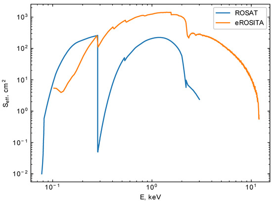
Figure 1.
Effective area of eROSITA and ROSAT telescopes versus photon energy. The data for eROSITA are presented under the assumption that signals from five out of seven telescopes pass through filters cutting off the soft part of the spectrum. The data for eROSITA are taken from the site https://wiki.mpe.mpg.de/eRosita/erocalib_calibration (accessed on 5 May 2022), for ROSAT — from [68].
To calculate count rates (CR) of the modeled sources we use the following expression:
where E is the photon energy, is the effective area of eROSITA, and are bounds of the range of sensitivity of the detector, r is the distance to the source, is the column density of hydrogen on the line of sight. The flux is reduced due to absorption by the factor (see the next subsection). To calculate the value, we use the equation and coefficients , , from [66]:
Finally, is the number of photons emitted from the whole surface of an isotropic source in the spectral interval per unit time for a distant observer (i.e., accounting for general relativistic effects).
We consider a source as potentially visible if its count rate exceeds the eROSITA detectability threshold 0.01 cts s. Detailed calculations of this limit can be found in [67]. Furthermore, this value corresponds to the limiting sensitivity flux erg s cm in the soft band [0.2–2.3] keV given in [7] assuming that the spectrum is a power-law with and no absorption is taken into account. This sensitivity corresponds to the total un-vignetted exposure equal to 1600 s. Effective (vignetted) exposure can be computed by dividing the total exposure by 1.88 in the soft band.
2.4. Interstellar absorption
Soft X-ray flux can be significantly weakened on the way to the Earth. To account for effects of propagation in the interstellar medium we need to specify a 3D distribution of the gas and then to calculate absorption.
The 3D distribution of the interstellar medium (separately for different constituents) in the whole Galactic volume is not well-known (see, e.g., discussion and references in [69]). Luckily, for our purposes we can neglect some details focusing on the general shape of the distribution. We proceed as follows. At first, we adopt distributions of molecular (H) and atomic (HI) hydrogen according to [70]. This provides us with the shape of the 3D distribution of the absorbing medium. For molecular hydrogen we have:
where cm is the number density of H molecules at the center of the Galaxy, kpc is the scale in the radial direction, and kpc is the scale height of the distribution.
Additionally, for atomic hydrogen:
Then, cm is the HI number density at the center of the Galaxy (i.e., at the center of the untruncated disk), kpc is the inner truncation radius, kpc is the radial scale, and kpc is the scaleheight of the distribution.
The total hydrogen column density is obtained by integration along the line of sight. It can be written as:
The integral in Equation (10) is calculated numerically.
We confront values of from Equation (10) integrated up to a very large distance (1 Mpc) with values provided by the online service at the Swift website in UK (https://www.swift.ac.uk/analysis/nhtot/index.php (accessed on 5 May 2022)) for Galactic [71]. This comparison is shown in Figure 2. To select directions in the sky we use coordinates of 100 synthetic sources with count rates >0.1 cts s. We find that our model is in good agreement with the data given by the web-tool.
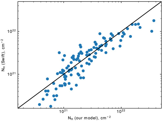
Figure 2.
Comparison of hydrogen column density throw the whole Galaxy computed using our model and obtained with the web-tool https://www.swift.ac.uk/analysis/nhtot/index.php (accessed on 5 May 2022) [71]. Solid diagonal line is the bisector. is shown for 100 directions corresponding to synthetic sources with CR cts s.
3. Results
We perform several simulations each including objects according to the model described above. Note that this leads to some statistical fluctuations in the results presented below, especially for bright sources, as analysed objects have a new random spatial distribution in each run.
We present our final results in the form of Log N – Log S distributions for different surface temperatures, Figure 3. Four values of the surface temperature of HOFNARs are used: K, K, K, and K. Obviously, for larger temperatures, eROSITA can detect more sources. The distributions for all temperatures are averaged over 10 runs.
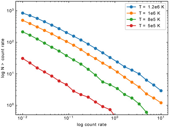
Figure 3.
Log N–Log S distributions (averaged over 10 runs, 2250 objects each) for different unredshifted surface temperatures of sources. The horizontal axis shows the count rate by eROSITA. Here we apply the XSPEC hydrogen atmosphere model nsatmos.
The Log N – Log S lines have a slope slightly flatter than . This is expected, as the sources are distributed in the disc, and at larger distances interstellar absorption becomes important. At the bright end the lines go steeper, asymptotically approaching the slope −3/2 for the brightest (and so—the closest) sources.
For the fiducial value K, about 500 sources are predicted above the detection limit 0.01 cts s. However, the identification of dim sources might be a very difficult task. Thus, the number of sources with count rate cts s might be a better reference point. Even for the minimal exposure s accounting for the vignetting coefficient 1.88, in 4 years of the survey this might provide photons which is enough for rough spectral classification (e.g., to identify the thermal spectrum and estimate the temperature). Additionally, we remind the reader that the survey was terminated early in 2022 and at the moment, it is unclear if the whole 4-year program can be completed. So, in addition to results on barely detectable sources, we also separately discuss sources with CR cts s, sometimes focusing particularly on them. For the surface temperature K the number of such sources is ∼100.
For surface temperatures K, the number of sources becomes too low to hope for successful identifications, unless the actual ratio of the number of HOFNARs to the number of MSPs is very close to the upper limit discussed above. For even lower temperatures perspectives to detect objects with the eROSITA all-sky survey becomes illusive.
In Figure 4 we show two distance distributions of HOFNARs with K and count rates >0.1 cts s and >0.01 cts s. It can be seen that a typical distance from the Sun is ∼3–8 kpc for the dimmer sources and ≲4–5 kpc – for the brighter.
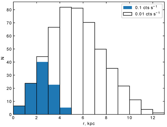
Figure 4.
Radial distributions (distance from the Sun) of sources with count rates cts s (unfilled histogram) and cts s (filled histogram) for K. The distributions are averaged over 10 runs.
Distribution in the sky is shown in Figure 5. As expected, bright nearby sources (lighter symbols) can be found at large Galactic latitudes, where it can be easier to identify them, but such objects are not numerous.
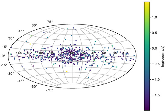
Figure 5.
Map of sources with count rates cts s in the Galactic coordinates for a single run with a total of 2250 sources. The surface temperature is K. Color of each circle corresponds to the count rate (see the bar on the right).
Concluding the presentation of our main results, we have to say that uncertainties in the absolute numbers of sources can reach a factor due to poor knowledge of several parameters, in the first place being the relative number of HOFNARs and MSPs.
4. Discussion
Population synthesis calculations presented above demonstrate that for realistic parameters, HOFNARs can be detected in the all-sky survey by eROSITA. Still, it is appropriate to discuss several issues related to non-detections in earlier surveys and difficulties in identifying HOFNARs among dim eROSITA sources.
4.1. Comparison with ROSAT
Before eROSITA, the best all-sky survey in soft X-rays was done by ROSAT. The final catalogue (2RXS) includes ∼135,000 items [72]. A significant fraction of these detections can be spurious, many sources are unidentified. The situation is much better for the bright source catalogue – RASS-BSC [73]. In this sample there are ∼18,000 sources with count rate cts s. A very high rate of identification is achieved in the ROSAT Bright Survey (RBS). This catalogue includes objects with count rate counts s and Galactic latitude [74]. It is useful to compare our model with this sample in order to be sure that we do not over-predict the number of bright sources.
We use our model and data on the response function of ROSAT ([68], see Figure 1) to calculate the number of HOFNARs and their distribution in the sky. The number of sources with ROSAT counts counts s and Galactic latitude for K on average is (the range is 0–3 in ∼10 realizations). For K we obtain 3 sources (the range 2–4), while for K predicted number of detected sources becomes ∼6 (the range 3–10). In the last case the predicted number of bright sources for ROSAT starts to be too big, as no objects which can be HOFNARs are identified in the RBS. This provides an opportunity to set an upper limit for the temperature of HOFNARs for our fiducial . Results for temperatures K do not contradict non-detection of HOFNAR candidates by ROSAT on the ∼ level, suggesting that our fiducial choice is, in fact, an upper limit imposed by ROSAT for the K. As in the case of predictions for detectability of HOFNARs by eROSITA, in calculations for the ROSAT observations this coefficient is the most uncertain quantity in our calculations. This uncertainty, which can easily reach a factor ∼2–3 (or even more), excludes any more precise limitation.
It is worth noting that the fact that ROSAT discovered seven X-ray Dim Isolated Neutron Stars (XDINSs), known as the Magnificent Seven [75,76], but not a single HOFNAR candidate should not be treated automatically as an argument that eROSITA should discover a much larger number of XDINSs than HOFNARs. The Magnificent Seven has its origin in the Gould Belt—the local ring-like structure made of young stars which encompasses the Sun [77]. So, the number density of young isolated NSs is enhanced in the Solar vicinity by a factor and does not represent the average number density in the Galactic disc. At larger distances in favourable conditions (, K) HOFNARs can be found in comparable number, or even outnumber XDINSs. Distinguishing between these two populations can be a difficult task. We briefly discuss some issues in the following subsection.
4.2. On Identification of HOFNARs in the X-ray Survey
As shown in Section 3, for our fiducial parameters (see Section 2) we expect detection of ∼500 HOFNARs in the completed eROSITA all-sky survey and ∼100 of them (i.e., ≲5% of the total HOFNAR population in the Galaxy) are expected to have rather high count rate s leading to a significant number of photons for rough spectral analysis. However, it is crucial not only to detect, but also to identify a source as a HOFNAR. Here we discuss some HOFNAR features, which can be used for identification. However, a detailed analysis of the identification strategy is beyond the scope of this paper.
Identification of sources of a given type can be difficult if there is another class of sources with very similar properties. In the case of HOFNARs, the main source of confusion can be due to young isolated NSs, which might be detected by eROSITA in a comparable number [78,79], and also due to qLMXBs.
Let us start with isolated NSs. The analysis of detectability of isolated NS with non-thermal radiation by eROSITA was recently carried out in [79]. It was found that among known sources eROSITA can detect ∼160 radio pulsars and ∼20 magnetars. Some isolated NSs—XDINSs and central compact objects (CCOs)—do not demonstrate non-thermal components in their spectra. It is expected that eROSITA will detect all known XDINSs and most CCOs. New discoveries are also expected. According to [78], eROSITA will be able to detect new XDINSs.
Hopefully, purely thermal X-ray emission allows us to discriminate HOFNARs from significant part of isolated NSs as many of them have non-thermal components in their spectra. A power law component is typically required to describe a high-energy tail in the X-ray emission of highly magnetized NSs (i.e., magnetars, see e.g., [80]) as well as many of NSs with ordinary magnetic fields (see e.g., [81] and references therein). It is also easy to identify CCOs (see Ref. [82] for a review) as they are located inside supernova remnants which is not expected for very old HOFNARs. Still, XDINSs require additional criteria to be discriminated from HOFNARs.
X-ray pulsations can be the first of such criteria. HOFNARs should have an almost isothermal surface and their emission should not pulsate at the spin rate, which should be high enough to allow the r-mode instability (≳200 Hz) [6]. Thus, detection of low-frequency pulsations excludes identification of a source as a HOFNAR. We remind the reader that pulsations of X-ray flux with periods 3–12 s are detected for at least six out of seven classical XDINSs [76]. Still, newly discovered XDINSs are expected to be dim objects with low count rate, even for eROSITA (in the survey mode). So, before they are observed with long exposures by X-ray observatories such as XMM-Newton, Chandra, eROSITA (in the pointing observation mode), and (in the near future) ATHENA, it might be impossible to detect pulsations.
The second criterion can be based on a detailed analysis of X-ray spectra, including their long-term variability. HOFNARs should be stable sources and no absorption features are predicted by hydrogen and helium atmosphere models for HOFNAR temperatures in the eROSITA energy range, see, e.g., [64]. This is in contrast with properties of the Magnificent Seven. So, the presence of such features in the data excludes the HOFNAR interpretation. It is crucial that in principle, this analysis can be done solely on the base of eROSITA data if enough photons are collected (see, e.g., [83] for analysis of some of the known XDINS); however, the contribution from other X-ray observatories is welcomed, as well as long dedicated eROSITA observations after the survey is completed.
An additional criterion of HOFNAR identification can be associated with X-ray polarization.2 However, the detection of polarization from dim X-ray sources is a challenging task. Future missions such as eXTP [86] can potentially succeed here.
Some other criteria are the following: absence of radio and gamma-ray counterparts demonstrating pulsations at non-millisecond periods, position of a source in the Galaxy (young NSs should be located in the regions with active star formations, while HOFNARs can be located at large Galactic latitudes, see Figure 5).
Finally, HOFNARs are born in LMXBs and the secondary component cannot be exhausted completely, yet. In this case, it can reveal itself in optical emission. For example, the X-ray source X5 in 47 Tucanae, which is a HOFNAR candidate [6], has a faint optical counterpart (, ) which can be interpreted as a companion not filling the Roche lobe [87]. Taking into account the distance to 47 Tuc (4.45 kpc) we can expect that if a HOFNAR has a secondary component with similar properties, then on average it should be detected (see Figure 4 for the expected distance distribution for detectable HOFNARs). Oppositely, even the brightest source among the Magnificent Seven—RX J1856.5-3754—at the distance ∼140 pc has [88,89], is clearly undetectable if located at ∼2–4 kpc distance. Correspondingly, many faint isolated cooling NS candidates (see, e.g., [90]) might not have optical counterparts. For example, the authors of [78] predict that just ∼25 among the expected ∼80 new XDINS (to be discovered by eROSITA) might have optical counterparts, which are expected to be very dim.
It can be extremely hard to discriminate HOFNARs from hot qLMXBs, because the main difference between these objects is the state of a companion star: for a qLMXB, the companion should fill the Roche lobe to allow (transient) accretion, required to maintain the NS temperature (e.g., [91] and references therein). Even known sources in globular clusters are still considered as candidates to both classes (see [6] for discussion). It is likely that important constraints for the qLMXB population potentially discovered by eROSITA can be obtained combining observational data on LMXBs with predictions of the disc instability model [92] (see [6] for a similar analysis for sources in globular clusters), but we leave these problems beyond this paper.
Furthermore, there can be statistical features supporting the hypothesis that the HOFNAR population is indeed detected. For example, if the temperature distribution of soft X-ray sources is clustered in a very narrow temperature range, as it would be natural for HOFNARs, but not for isolated NSs which continuously cool down and should have a smoother temperature distribution. In the absence of resonance stabilization of r-modes [41,41], temperatures of qLMXBs are determined by an average accretion rate (e.g., [91]) and also should have a smooth distribution. However, a practical application of this criterion requires a careful analysis of selection effects which clearly affects the observed population. Importance of such analysis, which is, however, beyond the scope of the present paper, is highlighted by the fact that temperatures of six XDINSs discovered by ROSAT lie in a relatively narrow range 85–102 eV [75].
Clearly, detection and identification of HOFNARs would be a magnificent result as they represent a new class of NSs with a specific source of thermal energy. It would not just confirm that the r-mode instability can be active in NSs, but also that it plays an important role in observational appearance of some LMXBs. Still, let us consider a possible negative case: none of X-ray sources discovered by eROSITA can be identified as a HOFNAR. It would be a clear indication that at least one of the assumptions used in our model (Section 2) is wrong.
The most direct interpretation of the negative result is the following: the number of Galactic HOFNARs with temperatures about the fiducial value K is very small. As long as ≲5% of HOFNARs should be detected above 0.1 cts s, a non-detection might limit the total Galactic number of HOFNARs with K by ≲ a few tens. This can have two (not mutually exclusive) explanations: either the probability of the birth of a HOFNAR in a LMXB is much lower than our fiducial value;3 and/or the life time of a HOFNAR at a temperature not much lower than the fiducial one is much smaller than the Galactic age. For example, the latter can be the case if LMXB evolution can lead to formation of heavy HOFNARs, with masses higher than the direct URCA threshold. In this case, HOFNARs would have a huge cooling power due to high neutrino luminosity. As far as HOFNAR evolution is governed by the following equation, see [6]
this would result in a short life time of a bright source. Here, is the rotational energy of a HOFNAR and t is time. Let us also remind the reader that LMXB evolution in globular clusters is more complicated due to close encounters and, in principle, this can lead to a more efficient production of observable HOFNARs than in the Galactic disc.
5. Conclusions
In this paper we presented a population model of HOFNARs—NSs originated in LMXBs and heated due to the r-mode instability. We demonstrate that in the framework of our fiducial model there are significant chances that from few tens up to several hundred of these sources will be detected in the eROSITA all-sky survey. If not, then important constraints can be placed on the properties and origin of such objects.
Author Contributions
A.I.C. initiated the study and supervised aspects of the model related to thermal properties of HOFNARs. A.D.K. and S.B.P. made the population synthesis model. The code was written by A.D.K., she also made calculations. E.M.K. and M.E.G. contributed to the discussion of results. M.E.G. has checked the calculations by independently written code. All authors have read and agreed to the published version of the manuscript.
Funding
A.D.K. and S.B.P. are supported by the Russian Science Foundation, grant 21-12-00141.
Data Availability Statement
Observational data used in this paper are quoted from the cited works. Data generated from computations are reported in the body of the paper. Additional data can be made available upon reasonable request.
Acknowledgments
We thank the referees for their useful comments.
Conflicts of Interest
The authors declare no conflict of interest.
Abbreviations
The following abbreviations are used in this manuscript:
| CCO | Central compact object |
| eROSITA | extended ROentgen Survey with an Imaging Telescope Array |
| HOFNAR | HOt and Fast Non Accreting Rotator |
| LXMB | Low-mass X-ray binary |
| MSP | Millisecond radio pulsar |
| NS | Neutron star |
| qLXMB | quiescent Low-mass X-ray binary |
| SRG | Spectrum-Roentgen-Gamma |
Notes
| 1 | Similar r-mode heating can take place in newly born neutron stars, if they rotate rapidly enough (e.g., [26,27,28,29]). However, they likely evolve very fast and quickly leave the r-mode instability region due to higher temperatures and, thus, stronger neutrino luminosity. |
| 2 | Imaging X-Ray Polarimetry Explorer mission—IXPE—was recently launched [84]. Effects of the magnetized vacuum were predicted to affect X-ray emission of XDINSs, e.g., [85]. |
| 3 | Here we treat as a newborn HOFNAR a NS which finishes the LMXB stage of evolution with active r-mode instability. |
References
- Shapiro, S.L.; Teukolsky, S.A. Black Holes, White Dwarfs, and Neutron Stars: The Physics of Compact Objects; Cornell University: Ithaca, NY, USA, 1983. [Google Scholar]
- Haensel, P.; Potekhin, A.; Yakovlev, D. Neutron Stars 1: Equation of State and Structure; Astrophysics and Space Science Library; Springer: Berlin/Heidelberg, Germny, 2007. [Google Scholar]
- Rezzolla, L.; Pizzochero, P.; Jones, D.I.; Rea, N.; Vidaña, I. (Eds.) The Physics and Astrophysics of Neutron Stars; Springer: Cham, Switzerland, 2018. [Google Scholar]
- Harding, A.K. The neutron star zoo. Front. Phys. 2013, 8, 679–692. [Google Scholar] [CrossRef]
- Abbott, B.P.; Abbott, R.; Abbott, T.D.; Acernese, F.; Ackley, K.; LIGO Scientific Collaboration; Virgo Collaboration. Properties of the Binary Neutron Star Merger GW170817. Phys. Rev. X 2019, 9, 011001. [Google Scholar] [CrossRef]
- Chugunov, A.I.; Gusakov, M.E.; Kantor, E.M. New possible class of neutron stars: Hot and fast non-accreting rotators. Mon. Not. R. Astron. Soc. 2014, 445, 385–391. [Google Scholar] [CrossRef][Green Version]
- Predehl, P.; Andritschke, R.; Arefiev, V.; Babyshkin, V.; Batanov, O.; Becker, W.; Böhringer, H.; Bogomolov, A.; Boller, T.; Borm, K.; et al. The eROSITA X-ray telescope on SRG. Astron. Astrophys. 2021, 647, A1. [Google Scholar] [CrossRef]
- Millisecond Pulsars. Available online: https://link.springer.com/book/10.1007/978-3-030-85198-9 (accessed on 15 June 2022).
- Bisnovatyi-Kogan, G.S.; Komberg, B.V. Possible evolution of a binary-system radio pulsar as an old object with a weak magnetic field. Sov. Astron. Lett. 1976, 2, 130–132. [Google Scholar]
- Alpar, M.A.; Cheng, A.F.; Ruderman, M.A.; Shaham, J. A new class of radio pulsars. Nature 1982, 300, 728–730. [Google Scholar] [CrossRef]
- Harding, A.K. The Emission Physics of Millisecond Pulsars. In Millisecond Pulsars; Bhattacharyya, S., Papitto, A., Bhattacharya, D., Eds.; Astrophysics and Space Science Library; Springer: Cham, Switzerland, 2022; Volume 465, pp. 57–85. [Google Scholar] [CrossRef]
- Reisenegger, A. Constraining Dense Matter Superfluidity through Thermal Emission from Millisecond Pulsars. Astrophys. J. 1997, 485, 313–318. [Google Scholar] [CrossRef]
- Kantor, E.M.; Gusakov, M.E. Long-lasting accretion-powered chemical heating of millisecond pulsars. Mon. Not. R. Astron. Soc. 2021, 508, 6118–6127. [Google Scholar] [CrossRef]
- Durant, M.; Kargaltsev, O.; Pavlov, G.G.; Kowalski, P.M.; Posselt, B.; van Kerkwijk, M.H.; Kaplan, D.L. The Spectrum of the Recycled PSR J0437-4715 and Its White Dwarf Companion. Astrophys. J. 2012, 746, 6. [Google Scholar] [CrossRef]
- Schwenzer, K.; Boztepe, T.; Güver, T.; Vurgun, E. X-ray bounds on the r-mode amplitude in millisecond pulsars. Mon. Not. R. Astron. Soc. 2017, 466, 2560–2569. [Google Scholar] [CrossRef]
- Chugunov, A.I.; Gusakov, M.E.; Kantor, E.M. R modes and neutron star recycling scenario. Mon. Not. R. Astron. Soc. 2017, 468, 291–304. [Google Scholar] [CrossRef]
- Bhattacharya, S.; Heinke, C.O.; Chugunov, A.I.; Freire, P.C.C.; Ridolfi, A.; Bogdanov, S. Chandra studies of the globular cluster 47 Tucanae: A deeper X-ray source catalogue, five new X-ray counterparts to millisecond radio pulsars, and new constraints to r-mode instability window. Mon. Not. R. Astron. Soc. 2017, 472, 3706–3721. [Google Scholar] [CrossRef]
- González-Caniulef, D.; Guillot, S.; Reisenegger, A. Neutron star radius measurement from the ultraviolet and soft X-ray thermal emission of PSR J0437-4715. Mon. Not. R. Astron. Soc. 2019, 490, 5848–5859. [Google Scholar] [CrossRef]
- Boztepe, T.; Göğüş, E.; Güver, T.; Schwenzer, K. Strengthening the bounds on the r-mode amplitude with X-ray observations of millisecond pulsars. Mon. Not. R. Astron. Soc. 2020, 498, 2734–2749. [Google Scholar] [CrossRef]
- Harding, A.K.; Muslimov, A.G. Pulsar Polar Cap Heating and Surface Thermal X-Ray Emission. I. Curvature Radiation Pair Fronts. Astrophys. J. 2001, 556, 987–1001. [Google Scholar] [CrossRef]
- Harding, A.K.; Muslimov, A.G. Pulsar Polar Cap Heating and Surface Thermal X-Ray Emission. II. Inverse Compton Radiation Pair Fronts. Astrophys. J. 2002, 568, 862–877. [Google Scholar] [CrossRef]
- Friedman, J.L.; Schutz, B.F. Lagrangian perturbation theory of nonrelativistic fluids. Astrophys. J. 1978, 221, 937–957. [Google Scholar] [CrossRef]
- Friedman, J.L.; Schutz, B.F. Secular instability of rotating Newtonian stars. Astrophys. J. 1978, 222, 281–296. [Google Scholar] [CrossRef]
- Andersson, N. A New Class of Unstable Modes of Rotating Relativistic Stars. Astrophys. J. 1998, 502, 708. [Google Scholar] [CrossRef]
- Chugunov, A.I. Radiation Driven Instability of Rapidly Rotating Relativistic Stars: Criterion and Evolution Equations Via Multipolar Expansion of Gravitational Waves. Publ. Astron. Soc. Australia 2017, 34, e046. [Google Scholar] [CrossRef][Green Version]
- Reisenegger, A.; Bonacic, A. Bulk viscosity, r-modes, and the early evolution of neutron stars. In Proceedings of the International Workshop on Pulsars, AXPs and SGRs Observed with BeppoSAX and Other Observatories, Marsala, Italy, 23–25 September 2002. [Google Scholar]
- Alford, M.G.; Schwenzer, K. Gravitational wave emission and spindown of young pulsars. Astrophys. J. 2014, 781, 26. [Google Scholar] [CrossRef]
- Routray, T.R.; Pattnaik, S.P.; Gonzalez-Boquera, C.; Viñas, X.; Centelles, M.; Behera, B. Influence of direct Urca on the r-mode spin down features of newborn neutron star pulsars. Phys. Scripta 2021, 96, 045301. [Google Scholar] [CrossRef]
- Lindblom, L.; Owen, B.J.; Morsink, S.M. Gravitational Radiation Instability in Hot Young Neutron Stars. Phys. Rev. Lett. 1998, 80, 4843–4846. [Google Scholar] [CrossRef]
- Popov, S.B.; Prokhorov, M.E. REVIEWS OF TOPICAL PROBLEMS: Population synthesis in astrophysics. Phys. Uspekhi 2007, 50, 1123–1146. [Google Scholar] [CrossRef]
- Ploeg, H.; Gordon, C.; Crocker, R.; Macias, O. Comparing the galactic bulge and galactic disk millisecond pulsars. J. Cosmology Astropart. Phys. 2020, 2020, 035. [Google Scholar] [CrossRef]
- Gonthier, P.L.; Harding, A.K.; Ferrara, E.C.; Frederick, S.E.; Mohr, V.E.; Koh, Y.M. Population Syntheses of Millisecond Pulsars from the Galactic Disk and Bulge. Astrophys. J. 2018, 863, 199. [Google Scholar] [CrossRef]
- Story, S.A.; Gonthier, P.L.; Harding, A.K. Population Synthesis of Radio and γ-Ray Millisecond Pulsars from the Galactic Disk. Astrophys. J. 2007, 671, 713–726. [Google Scholar] [CrossRef]
- Haskell, B. R-modes in neutron stars: Theory and observations. Int. J. Mod. Phys. E 2015, 24, 1541007. [Google Scholar] [CrossRef]
- Kantor, E.M.; Gusakov, M.E.; Dommes, V.A. Constraining Neutron Superfluidity with R -Mode Physics. Phys. Rev. Lett. 2020, 125, 151101. [Google Scholar] [CrossRef] [PubMed]
- Kantor, E.M.; Gusakov, M.E.; Dommes, V.A. Resonance suppression of the r-mode instability in superfluid neutron stars: Accounting for muons and entrainment. Phys. Rev. D 2021, 103, 023013. [Google Scholar] [CrossRef]
- Kraav, K.Y.; Gusakov, M.E.; Kantor, E.M. Non-analytic behavior of the relativistic r-modes in slowly rotating neutron stars. arXiv 2021, arXiv:2112.01171. [Google Scholar]
- Heinke, C.O.; Grindlay, J.E.; Lloyd, D.A.; Edmonds, P.D. X-Ray Studies of Two Neutron Stars in 47 Tucanae: Toward Constraints on the Equation of State. Astrophys. J. 2003, 588, 452–463. [Google Scholar] [CrossRef]
- Bogdanov, S.; Heinke, C.O.; Özel, F.; Güver, T. Neutron Star Mass-Radius Constraints of the Quiescent Low-mass X-Ray Binaries X7 and X5 in the Globular Cluster 47 Tuc. Astrophys. J. 2016, 831, 184. [Google Scholar] [CrossRef]
- Heinke, C.O.; Grindlay, J.E.; Edmonds, P.D. Three Additional Quiescent Low-Mass X-Ray Binary Candidates in 47 Tucanae. Astrophys. J. 2005, 622, 556–564. [Google Scholar] [CrossRef]
- Gusakov, M.E.; Chugunov, A.I.; Kantor, E.M. Instability Windows and Evolution of Rapidly Rotating Neutron Stars. Phys. Rev. Lett. 2014, 112, 151101. [Google Scholar] [CrossRef] [PubMed]
- Gusakov, M.E.; Chugunov, A.I.; Kantor, E.M. Explaining observations of rapidly rotating neutron stars in low-mass x-ray binaries. Phys. Rev. D 2014, 90, 063001. [Google Scholar] [CrossRef]
- Martsen, A.R.; Ransom, S.M.; DeCesar, M.E.; Freire, P.C.C.; Hessels, J.W.T.; Ho, A.Y.Q.; Lynch, R.S.; Stairs, I.H.; Wang, Y. Pulse Profiles and Polarization of Terzan 5 Pulsars. arXiv 2022, arXiv:2204.06158. [Google Scholar]
- Ivanova, N.; Heinke, C.O.; Rasio, F.A.; Belczynski, K.; Fregeau, J.M. Formation and evolution of compact binaries in globular clusters—II. Binaries with neutron stars. Mon. Not. R. Astron. Soc. 2008, 386, 553–576. [Google Scholar] [CrossRef]
- Pfahl, E.; Rappaport, S.; Podsiadlowski, P. The Galactic Population of Low- and Intermediate-Mass X-Ray Binaries. Astrophys. J. 2003, 597, 1036–1048. [Google Scholar] [CrossRef]
- Levin, Y.; Ushomirsky, G. Crust core coupling and r mode damping in neutron stars: A Toy model. Mon. Not. Roy. Astron. Soc. 2001, 324, 917. [Google Scholar] [CrossRef]
- Lindblom, L.; Owen, B.J. Effect of hyperon bulk viscosity on neutron-star r-modes. Phys. Rev. D 2002, 65, 063006. [Google Scholar] [CrossRef]
- Glampedakis, K.; Andersson, N. Crust-core coupling in rotating neutron stars. Phys. Rev. D 2006, 74, 044040. [Google Scholar] [CrossRef]
- Glampedakis, K.; Andersson, N. Ekman layer damping of r modes revisited. Mon. Not. R. Astron. Soc. 2006, 371, 1311–1321. [Google Scholar] [CrossRef][Green Version]
- Haskell, B.; Andersson, N.; Passamonti, A. r modes and mutual friction in rapidly rotating superfluid neutron stars. Mon. Not. R. Astron. Soc. 2009, 397, 1464–1485. [Google Scholar] [CrossRef]
- Alford, M.G.; Mahmoodifar, S.; Schwenzer, K. Viscous damping of r-modes: Small amplitude instability. Phys. Rev. D 2012, 85, 024007. [Google Scholar] [CrossRef]
- Alford, M.G.; Schwenzer, K. What the Timing of Millisecond Pulsars Can Teach us about Their Interior. Phys. Rev. Lett. 2014, 113, 251102. [Google Scholar] [CrossRef] [PubMed]
- Haskell, B.; Glampedakis, K.; Andersson, N. A new mechanism for saturating unstable r modes in neutron stars. Mon. Not. R. Astron. Soc. 2014, 441, 1662–1668. [Google Scholar] [CrossRef]
- Kokkotas, K.D.; Schwenzer, K. R-mode astronomy. Eur. Phys. J. A 2016, 52, 38. [Google Scholar] [CrossRef]
- Pattnaik, S.P.; Routray, T.R.; Viñas, X.; Basu, D.N.; Centelles, M.; Madhuri, K.; Behera, B. Influence of the nuclear matter equation of state on the r-mode instability using the finite-range simple effective interaction. J. Phys. G 2018, 45, 055202. [Google Scholar] [CrossRef]
- Ofengeim, D.D.; Gusakov, M.E.; Haensel, P.; Fortin, M. R-mode stabilization in neutron stars with hyperon cores. J. Phys. Conf. Seri. 2019, 1400, 022029. [Google Scholar] [CrossRef]
- Ofengeim, D.D.; Gusakov, M.E.; Haensel, P.; Fortin, M. Bulk viscosity in neutron stars with hyperon cores. Phys. Rev. D 2019, 100, 103017. [Google Scholar] [CrossRef]
- Chen, H.L.; Chen, X.; Tauris, T.M.; Han, Z. Formation of Black Widows and Redbacks—Two Distinct Populations of Eclipsing Binary Millisecond Pulsars. Astrophys. J. 2013, 775, 27. [Google Scholar] [CrossRef]
- Parfrey, K.; Spitkovsky, A.; Beloborodov, A.M. Torque Enhancement, Spin Equilibrium, and Jet Power from Disk-Induced Opening of Pulsar Magnetic Fields. Astrophys. J. 2016, 822, 33. [Google Scholar] [CrossRef]
- Bhattacharyya, S.; Chakrabarty, D. The Effect of Transient Accretion on the Spin-up of Millisecond Pulsars. Astrophys. J. 2017, 835, 4. [Google Scholar] [CrossRef]
- Özel, F.; Freire, P. Masses, Radii, and the Equation of State of Neutron Stars. Annu. Rev. Astron. Astrophys. 2016, 54, 401–440. [Google Scholar] [CrossRef]
- Horvath, J.E.; Rocha, L.S.; Bernardo, A.L.C.; de Avellar, M.G.B.; Valentim, R. Birth events, masses and the maximum mass of Compact Stars. arXiv 2020, arXiv:2011.08157. [Google Scholar]
- Heinke, C.O.; Rybicki, G.B.; Narayan, R.; Grindlay, J.E. A Hydrogen Atmosphere Spectral Model Applied to the Neutron Star X7 in the Globular Cluster 47 Tucanae. Astrophys. J. 2006, 644, 1090–1103. [Google Scholar] [CrossRef]
- Zavlin, V.E.; Pavlov, G.G.; Shibanov, Y.A. Model neutron star atmospheres with low magnetic fields. I. Atmospheres in radiative equilibrium. Astron. Astrophys. 1996, 315, 141–152. [Google Scholar]
- Merloni, A.; Predehl, P.; Becker, W.; Böhringer, H.; Boller, T.; Brunner, H.; Brusa, M.; Dennerl, K.; Freyberg, M.; Friedrich, P.; et al. eROSITA Science Book: Mapping the Structure of the Energetic Universe. arXiv 2012, arXiv:1209.3114. [Google Scholar]
- Morrison, R.; McCammon, D. Interstellar photoelectric absorption cross sections, 0.03–10 keV. Astrophys. J. 1983, 270, 119–122. [Google Scholar] [CrossRef]
- Khokhryakova, A.D.; Biryukov, A.V.; Popov, S.B. Observability of Single Neutron Stars at SRG/eROSITA. Astronomy Reports 2021, 65, 615–630. [Google Scholar] [CrossRef]
- Pfeffermann, E.; Briel, U.G.; Hippmann, H.; Kettenring, G.; Metzner, G.; Predehl, P.; Reger, G.; Stephan, K.H.; Zombeck, M.; Chappell, J.; et al. The focal plane instrumentation of the ROSAT Telescope. In Soft X-Ray Optics and Technology; Society of Photo-Optical Instrumentation Engineers (SPIE) Conference Series: Bellingham, WA, USA, 1987; Volume 733, p. 519. [Google Scholar]
- Sofue, Y.; Nakanishi, H. Three-dimensional distribution of the ISM in the Milky Way Galaxy. IV. 3D molecular fraction and Galactic-scale H I-to-H2 transition. Publ. Astron. Soc. Jpn. 2016, 68, 63. [Google Scholar] [CrossRef]
- Misiriotis, A.; Xilouris, E.M.; Papamastorakis, J.; Boumis, P.; Goudis, C.D. The distribution of the ISM in the Milky Way. A three-dimensional large-scale model. Astron. Astrophys. 2006, 459, 113–123. [Google Scholar] [CrossRef]
- Willingale, R.; Starling, R.L.C.; Beardmore, A.P.; Tanvir, N.R.; O’Brien, P.T. Calibration of X-ray absorption in our Galaxy. Mon. Not. R. Astron. Soc. 2013, 431, 394–404. [Google Scholar] [CrossRef]
- Boller, T.; Freyberg, M.J.; Trümper, J.; Haberl, F.; Voges, W.; Nandra, K. Second ROSAT all-sky survey (2RXS) source catalogue. Astron. Astrophys. 2016, 588, A103. [Google Scholar] [CrossRef]
- Voges, W.; Aschenbach, B.; Boller, T.; Bräuninger, H.; Briel, U.; Burkert, W.; Dennerl, K.; Englhauser, J.; Gruber, R.; Haberl, F.; et al. The ROSAT all-sky survey bright source catalogue. Astron. Astrophys. 1999, 349, 389–405. [Google Scholar]
- Schwope, A.; Hasinger, G.; Lehmann, I.; Schwarz, R.; Brunner, H.; Neizvestny, S.; Ugryumov, A.; Balega, Y.; Trümper, J.; Voges, W. The ROSAT Bright Survey: II. Catalogue of all high-galactic latitude RASS sources with PSPC countrate CR > 0.2 s−1. Astron. Nachr. 2000, 321, 1–52. [Google Scholar] [CrossRef]
- Haberl, F. The magnificent seven: Magnetic fields and surface temperature distributions. Astrophys. Space Sci. 2007, 308, 181–190. [Google Scholar] [CrossRef]
- Turolla, R. Isolated Neutron Stars: The Challenge of Simplicity; Becker, W., Ed.; Astrophysics and Space Science Library; Springer: Cham, Switzerland, 2009; Volume 357, p. 141. [Google Scholar] [CrossRef]
- Popov, S.B.; Colpi, M.; Prokhorov, M.E.; Treves, A.; Turolla, R. Young isolated neutron stars from the Gould Belt. Astron. Astrophys. 2003, 406, 111–117. [Google Scholar] [CrossRef]
- Pires, A.M.; Schwope, A.D.; Motch, C. Follow-up of isolated neutron star candidates from the eROSITA survey. Astron. Nachr. 2017, 338, 213–219. [Google Scholar] [CrossRef]
- Khokhriakova, A.D.; Biryukov, A.V.; Popov, S.B. Observability of isolated neutron stars at SRG/eROSITA. arXiv 2022, arXiv:2201.07639. [Google Scholar]
- Olausen, S.A.; Kaspi, V.M. The McGill Magnetar Catalog. Astrophys. J. Suppl. 2014, 212, 6. [Google Scholar] [CrossRef]
- Potekhin, A.Y.; Zyuzin, D.A.; Yakovlev, D.G.; Beznogov, M.V.; Shibanov, Y.A. Thermal luminosities of cooling neutron stars. Mon. Not. R. Astron. Soc. 2020, 496, 5052–5071. [Google Scholar] [CrossRef]
- De Luca, A. Central compact objects in supernova remnants. arXiv 2017, arXiv:1711.07210. [Google Scholar] [CrossRef]
- Mancini Pires, A.; Schwope, A.; Kurpas, J. Deep eROSITA observations of the “magnificent seven” isolated neutron stars. arXiv 2022, arXiv:2202.06793. [Google Scholar]
- Weisskopf, M.C.; Soffitta, P.; Baldini, L.; Ramsey, B.D.; O’Dell, S.L.; Romani, R.W.; Matt, G.; Deininger, W.D.; Baumgartner, W.H.; Bellazzini, R.; et al. The Imaging X-Ray Polarimetry Explorer (IXPE): Pre-Launch. arXiv 2021, arXiv:2112.01269. [Google Scholar]
- Gonzalez Caniulef, D.; Zane, S.; Taverna, R.; Turolla, R.; Wu, K. Polarized thermal emission from X-ray dim isolated neutron stars: The case of RX J1856.5-3754. Mon. Not. R. Astron. Soc. 2016, 459, 3585–3595. [Google Scholar] [CrossRef]
- Zhang, S.; Santangelo, A.; Feroci, M.; Xu, Y.; Lu, F.; Chen, Y.; Feng, H.; Zhang, S.; Brandt, S.; Hernanz, M.; et al. The enhanced X-ray Timing and Polarimetry mission—eXTP. Sci. ChinaPhys.Mech. Astron. 2019, 62, 29502. [Google Scholar] [CrossRef]
- Edmonds, P.D.; Heinke, C.O.; Grindlay, J.E.; Gilliland, R.L. Hubble Space Telescope Detection of a Quiescent Low-Mass X-Ray Binary Companion in 47 Tucanae. Astrophys. J. Lett. 2002, 564, L17–L20. [Google Scholar] [CrossRef]
- van Kerkwijk, M.H.; Kulkarni, S.R. Optical spectroscopy and photometry of the neutron star <ASTROBJ>RX J1856.5-3754</ASTROBJ>. Astron. Astrophys. 2001, 378, 986–995. [Google Scholar]
- Ho, W.C.G.; Kaplan, D.L.; Chang, P.; van Adelsberg, M.; Potekhin, A.Y. Magnetic hydrogen atmosphere models and the neutron star RX J1856.5-3754. Mon. Not. R. Astron. Soc. 2007, 375, 821–830. [Google Scholar] [CrossRef]
- Rigoselli, M.; Mereghetti, S.; Tresoldi, C. Candidate isolated neutron stars in the 4XMM-DR10 catalogue of X-ray sources. Mon. Not. R. Astron. Soc. 2022, 509, 1217–1226. [Google Scholar] [CrossRef]
- Potekhin, A.Y.; Chugunov, A.I.; Chabrier, G. Thermal evolution and quiescent emission of transiently accreting neutron stars. Astron. Astrophys. 2019, 629, A88. [Google Scholar] [CrossRef]
- Lasota, J.P. The disc instability model of dwarf novae and low-mass X-ray binary transients. New Astron. Rev. 2001, 45, 449–508. [Google Scholar] [CrossRef]
Publisher’s Note: MDPI stays neutral with regard to jurisdictional claims in published maps and institutional affiliations. |
© 2022 by the authors. Licensee MDPI, Basel, Switzerland. This article is an open access article distributed under the terms and conditions of the Creative Commons Attribution (CC BY) license (https://creativecommons.org/licenses/by/4.0/).