Modified Equations of State for Dark Energy and Observational Limitations

Abstract

Cosmological models with variable and modified equations of state for dark energy are confronted with observational data, including Type Ia supernovae, Hubble parameter data $H\left(z\right)$ from different sources, and observational manifestations of cosmic microwave background radiation (CMB). We consider scenarios generalizing the $\Lambda$CDM, wCDM, and Chevallier–Polarski–Linder (CPL) models with nonzero curvature and compare their predictions. The most successful model with the dark energy equation of state $w=w_0+w_1(1-a^2)/2$ was studied in detail. These models are interesting in possibly alleviating the Hubble constant $H_0$ tension, but they achieved a modest success in this direction with the considered observational data.

1. Introduction

In modern cosmology based on recent observational data, our Universe includes dominating fractions of dark energy and dark matter, whereas all kinds of visible matter fill about 4% in total energy balance nowadays. The latest estimations of Planck collaboration [1,2] predict about 70% fraction of dark energy, if we apply the standard $\Lambda$CDM model, where dark energy may be represented as the cosmological constant $\Lambda$ or as a matter with density ${\rho }_x$ and pressure $p_x=-{\rho }_x$. Almost all remaining part of matter in this model is cold dark matter with close to zero pressure. Because of the last property, it is convenient to consider cold dark matter together with visible baryonic matter, where the unified density is ${\rho }_m={\rho }_c+{\rho }_b$. One should also add the radiation component including relativistic species (neutrinos) with $p_r=\frac{1}{3}{\rho }_r$, which was sufficient before and during the recombination era, but is is almost negligible now.

The $\Lambda$CDM model successfully describes numerous observations, including Type Ia supernovae (SNe Ia) data, estimates of the Hubble parameter $H\left(z\right)$, manifestations of baryonic acoustic oscillations (BAO), cosmic microwave background radiation (CMB), and other data [1,2]. However this model does not explain the nature of dark energy, the small observable value of the phenomenological constant $\Lambda$ and the approximate equality ${\rho }_x$ and ${\rho }_m$ now (although these densities evolve differently).

Another essential problem in the $\Lambda$CDM model is the tension between Planck estimations of the Hubble constant $H_0=67.37\pm 0.54$ km /(s·Mpc) [2] (2018) and measurements of SH0ES group in the Hubble Space Telescope $H_0=73.2\pm 1.3$ km s${}^{-1}$ Mpc${}^{-1}$ [3] (2020) or $H_0=73.3\pm 1.04$ km s${}^{-1}$ Mpc${}^{-1}$ [4] (2021).

The Planck estimations [1,2] are based on the $\Lambda$CDM model and the Planck satellite measurements of the CMB anisotropy and power spectra related to the early Universe at redshifts $z\sim 1000$, whereas the SH0ES method uses local distance ladder measurements of Cepheids in our Galaxy [3] and in nearest galaxies, in particular, in the Large Magellanic Cloud [5], that implies z close to 0 (the late Universe). This $H_0$ tension has not diminished during the last years, and now it exceeds $4\sigma$.

Cosmologists suggested numerous scenarios for solving the mentioned problems with dark energy and the $H_0$ tension; they include modifications of early or late dark energy, dark energy with extra degrees of freedom, models with interaction in dark sector, models with extra relativistic species, viscosity, modified gravity including $F\left(R\right)$ theories, and other models (see reviews [6,7,8,9,10] and papers [11,12,13,14,15,16,17,18,19,20,21]).

In this paper, we consider cosmological scenarios with modified equation of state (EoS) for dark energy; they generalize the $\Lambda$CDM model and its simplest extensions: the wCDM model with EoS

$$p_x=w{\rho }_x,w=\mathrm{const}$$

(1)

and the models with variable EoS

$$p_x=w\left(a\right){\rho }_x,$$

(2)

where w depends on the scale factor a. The class (2) includes the following well-known dark energy equations of state: the linear model [22]

$$w=w_0+w_1(a^{-1}-1)=w_0+w_{1}z;$$

(3)

Chevallier–Polarski–Linder (CPL) parametrization [23,24]

$$w=w_0+w_1(1-a)=w_0+w_1\frac{z}{1+z}$$

(4)

and (their generalization) Barboza–Alcaniz–Zhu–Silva (BAZS) EoS [25]

$$w=w_0+w_1\frac{1-a^{\beta }}{\beta }=w_0+w_1\frac{1-{(1+z)}^{-\beta }}{\beta }.$$

(5)

Here, the scale factor a is normalized, so $a\left(t_0\right)=1$ at the present time $t_0$; a is connected with redshift z: $a={(1+z)}^{-1}$. Obviously, BAZS parametrization (5) transforms into CPL EoS (4) at $\beta =1$, into the linear EoS (3) if $\beta =-1$ and into the logarithmic EoS $w=w_0+w_{1}log(1+z),$ if $\beta \to 0$.

For all mentioned equations of state, one can integrate the continuity equation for non-interacting dark energy:

$${\dot{\rho }}_x=-3H({\rho }_x+p_x).$$

(6)

In this paper, we explore the above scenarios and suggest the following generalization of BAZS EoS:

$$w=w_0+w_1\frac{1-a^{\beta }}{\beta }{a}^{\gamma }.$$

(7)

We test these models, confronting them with the following observational data: Type Ia supernovae data (SNe Ia) from the Pantheon sample survey [26], data extracted from Planck 2018 observations [2,27] of cosmic microwave background radiation (CMB), and estimations of the Hubble parameter $H\left(z\right)=\dot{a}/a$ for different redshifts z (the dot means $\frac{d}{dt}$). We use $H\left(z\right)$ data from two sources: (a) from cosmic chronometers, that is, measured from differential ages of galaxies, and (b) estimates of $H\left(z\right)$ obtained from line-of-sight baryonic acoustic oscillations (BAO) data.

This paper is organized as follows. In the next section, we describe $H\left(z\right)$, SNe Ia, and CMB observational data analyzed here. Section 3 is devoted to dynamics and free model parameters for scenarios (1)–(7). In Section 4 we analyze the results of our calculations for these models, and estimate values of model parameters including the Hubble constant $H_0$, and in Section 5 we discuss the results and their possible applications for alleviating the Hubble constant tension problem.

2. Observational Data

Observational data should be described by the considered cosmological models. For each model, we calculate the best fit for its free parameters from the abovementioned data sources: (a) Type Ia supernovae (SNe Ia) data from Pantheon sample [26], (b) CMB data from Planck 2018 [2,27], and (c) estimates of the Hubble parameter $H\left(z\right)$ from cosmic chronometers and line-of-sight BAO data.

The Pantheon sample database [26] for SNe Ia contains $N_{SN}=1048$ data points of distance moduli ${\mu }_i^{\mathrm{obs}}$ at redshifts $z_i$ in the range $0<z_i<1.92$. We compare them with theoretical values by minimizing the ${\chi }^2$ function:

$${\chi }_{\mathrm{SN}}^2({\theta }_1,\cdots )=\underset{H_0}{min}\sum _{i,j=1}^{N_{\mathrm{SN}}}\Delta {\mu }_i{\left(C_{\mathrm{SN}}^{-1}\right)}_{ij}\Delta {\mu }_j,\Delta {\mu }_i={\mu }^{\mathrm{th}}(z_i,{\theta }_1,\cdots )-{\mu }_i^{\mathrm{obs}},$$

(8)

Here, ${\theta }_j$ are free model parameters, $C_{\mathrm{SN}}$ is the covariance matrix [26], and the distance moduli ${\mu }^{\mathrm{th}}$ are expressed via the luminosity distance $D_L$ depending on the spacial curvature fraction ${\Omega }_k$ and the Hubble parameter $H\left(z\right)$:

$${\mu }^{\mathrm{th}}\left(z\right)=m_B\left(z\right)-M_B=5{log}_{10}\frac{D_L\left(z\right)}{10pc},D_L\left(z\right)=(1+z)D_M,$$

$$D_M\left(z\right)=\frac{c}{H_0}{S}_k\left(H_0\underset{0}{\overset{z}{\int }}\frac{d\tilde{z}}{H\left(\tilde{z}\right)}\right),S_k\left(x\right)=\left\{\begin{array}{cc}sinh\left(x\sqrt{{\Omega }_k}\right)/\sqrt{{\Omega }_k},\hfill & {\Omega }_k>0,\hfill \\ x,\hfill & {\Omega }_k=0,\hfill \\ sin\left(x\sqrt{|{\Omega }_k|}\right)/\sqrt{|{\Omega }_k|}.\hfill & {\Omega }_k<0,\hfill \end{array}\right.$$

Here, $m_B$ is a supernova apparent magnitude, and $M_B$ is its absolute magnitude. The distance moduli ${\mu }^{\mathrm{th}}$ are not Hubble-free and depend on the Hubble constant $H_0=H\left(t_0\right)$ (via the summand $-5{log}_{10}{H}_0$). On the other hand, ${\mu }_i^{\mathrm{obs}}$ is essentially connected with the absolute magnitude $M_B$ and calculated with corrections coming from deviations of lightcurve shape, SN Ia color, and mass of a host galaxy [26,28]. In the Pantheon sample, these corrections and the connected pair $(H_0,M_B)$ were considered as nuisance parameters, in particular: “Using only SNe, there is no constraint on $H_0$ since $H_0$ and $M_B$ are degenerate” [26]. We cannot divide uncertainties in the Hubble constant $H_0$ and possible uncertainties in $M_B$ [29,30,31].

Due to these reasons, we have to consider $H_0$ in Equation (8) as a nuisance parameter, its estimations cannot be obtained from ${\chi }_{\mathrm{SN}}^2$, and we minimize this function over $H_0$ [17,18,19,20,21]. However, SHe Ia data in ${\chi }_{\mathrm{SN}}^2$ is important for fitting other model parameters.

Unlike SNe Ia Pantheon data, the CMB observations are related to the photon-decoupling epoch near $z_{*}\simeq 1090$. We use the following parameters extracted from Planck 2018 CMB observations [2,20,27]:

$$x=\left(R,{\ell }_A,{\omega }_b\right),R=\sqrt{{\Omega }_m^0}\frac{H_0{D}_M\left(z_{*}\right)}{c},{\ell }_A=\frac{\pi D_M\left(z_{*}\right)}{r_s\left(z_{*}\right)},{\omega }_b={\Omega }_b^0{h}^2$$

(9)

and their estimations for the non-flat $\Lambda$CDM + ${\Omega }_k$ model [27]:

$$x^{\mathrm{Pl}}=\left(R^{\mathrm{Pl}},{\ell }_A^{\mathrm{Pl}},{\omega }_b^{\mathrm{Pl}}\right)=\left(1.7429\pm 0.0051,301.409\pm 0.091,0.0226\pm 0.00017\right).$$

(10)

Considering the flat case (${\Omega }_k=0$) of these models, we use the flat wCDM data [27]. The comoving sound horizon $r_s$ at $z_{*}$ is calculated as the integral

$$r_s\left(z_{*}\right)={\int }_{z_{*}}^{\infty }\frac{c_s\left(\tilde{z}\right)}{H\left(\tilde{z}\right)}d\tilde{z}=\frac{1}{\sqrt{3}}{\int }_0^{1/(1+z_{*})}\frac{da}{a^{2}H\left(a\right)\sqrt{1+\left[3{\Omega }_b^0/\left(4{\Omega }_{\gamma }^0\right)\right]a}}$$

(11)

with the fitting formula from Refs. [27,32] for the value $z_{*}$. The resulting ${\chi }^2$ function is

$${\chi }_{\mathrm{CMB}}^2=\underset{{\omega }_b}{min}\Delta \mathbf{x}·C_{\mathrm{CMB}}^{-1}{\left(\Delta \mathbf{x}\right)}^T,\Delta x=x-x^{\mathrm{Pl}},$$

(12)

where we minimize over the normalized baryon fraction ${\omega }_b^0$ to diminish the effective number $N_p$ of free model parameters. The covariance matrix $C_{\mathrm{CMB}}=∥{\tilde{C}}_{ij}{\sigma }_i{\sigma }_j∥$ and other details are described in papers [17,27].

In this paper, we use the Hubble parameter data $H\left(z\right)$ obtained from two different sources [17,18,19,20,21,33]. The first one is the cosmic chronometers (CC), in other words, estimations of $H\left(z\right)$ via differences of ages $\Delta t$ for galaxies with close redshifts $\Delta z$ and the formula

$$H\left(z\right)=\frac{\dot{a}}{a}\simeq -\frac{1}{1+z}\frac{\Delta z}{\Delta t}.$$

Here, we include 31 CC $H\left(z\right)$ data points from Refs. [34,35,36,37,38,39,40] used earlier in papers [17,18,19,20] and the recent estimate from Ref. [41]; they are shown in Table 1.

These 32 CC data points need a covariance matrix of systematic uncertainties connected with a choice of initial mass function, metallicity, star formation history, stellar population synthesis models, and other factors [42,43].

We describe these uncertainties as corrections $\Delta C_{\mathrm{H}}$ to the diagonal covariance matrix $C_{\mathrm{H}}^{\mathrm{d}}=\mathrm{diag}\left\{{\sigma }_i^{-2}\right\}$ (from Table 1) taking into account their diagonal terms in the form [42]

$${(\Delta C_{\mathrm{H}})}_{ii}={\left[\eta \left(z_i\right)H\left(z_i\right)\right]}^2.$$

Here, $\eta \left(z\right)$ is a mean percentage bias depending on redshift z. We consider “the best-case scenario” from the paper [42] for $\eta \left(z\right)$ and include these contributions of stellar population synthesis and metallicity omitting the non-diagonal terms $\Delta {\left(C_{\mathrm{H}}\right)}_{ij}$ (they are negligible for metallicity [43]).

The second source of $H\left(z\right)$ estimates is the baryon acoustic oscillation (BAO) data along the line-of-sight direction. We use here 36 $H_{\mathrm{BAO}}\left(z\right)$ data points from Refs. [44,45,46,47,48,49,50,51,52,53,54,55,56,57,58] (see Table 1). They were considered earlier in Ref. [21].

Some of the $H\left(z\right)$ measurements [44,45,46,47,48,49,50,51,52,53,54,55,56,57,58] in Table 1 used the same or overlapping large-scale structure data, so these H estimates for close redshifts z may be in duplicate. It concerns, for example, measurements of Delubac et al. [51], Font-Ribera et al. [50], uses quasars with Lyman-$\alpha$ forest from Data Release 11 SDSS-III survey; estimates of Alam et al. [54], Wang et al. [53], Bautista et al. [55], and Bourboux et al. [56] were made with data from or DR12 of SDSS-III etc. To avoid this doubling, we multiply the errors ${\sigma }_i$ by $\sqrt{2}$ for $H_{\mathrm{BAO}}$ estimates in Table 1 with close z, data, and methods.

Note that $H_{\mathrm{BAO}}$ estimates in Table 1 should be multiplied by the factor $r_d^{\mathrm{fid}}/r_d$, where fiducial values $r_d^{\mathrm{fid}}$ of the sound horizon size $r_d=r_s\left(z_d\right)$ at the drag epoch vary from 147.33 Mpc to 157.2 Mpc for different authors [44,45,46,47,48,49,50,51,52,53,54,55,56,57,58]. We include this correction to errors ${\sigma }_i$ quadratically, comparing deviations of $r_d^{\mathrm{fid}}$ with $r_s\left(z_d\right)$ calculated with Formula (11) for a considered model.

For any cosmological model we calculate the ${\chi }^2$ function

$${\chi }_H^2({\theta }_1,\cdots )=\sum _{j=1}^{N_H}{\left[\frac{H(z_j,{\theta }_1,\cdots )-H^{obs}\left(z_j\right)}{{\sigma }_j}\right]}^2$$

(13)

by using (a) only CC $H\left(z\right)$ data and (b) the full set CC + $H_{\mathrm{BAO}}$ data. Note that $H_{\mathrm{BAO}}$ data points are correlated with BAO angular distances considered in the previous papers [18,19,20]). Thus, here, we do not use data with BAO angular distances, to avoid any correlation.

Table 1. $H\left(z\right)$ data from cosmic chronometers (CC) [34,35,36,37,38,39,40,41] and line-of-sight BAO [44,45,46,47,48,49,50,51,52,53,54,55,56,57,58].

CC Data				${\mathit{H}}_{\mathbf{BAO}}$ Data
$\mathit{z}$	$\mathit{H}\left(\mathit{z}\right)$	$\mathbf{\sigma }$	Refs	$\mathit{z}$	$\mathit{H}\left(\mathit{z}\right)$	$\mathbf{\sigma }$	Refs
0.070	69	19.6	Zhang 14	0.240	79.69	2.992	Gaztañaga 09
0.090	69	12	Simon 05	0.30	81.7	6.22	Oka 14
0.120	68.6	26.2	Zhang 14	0.31	78.18	4.74	Wang 17
0.170	83	8	Simon 05	0.34	83.8	3.66	Gaztañaga 09
0.1791	75	4	Moresco 12	0.350	82.7	9.13	ChuangW 13
0.1993	75	5	Moresco 12	0.36	79.94	3.38	Wang 17
0.200	72.9	29.6	Zhang 14	0.38	81.5	1.9	Alam 17
0.270	77	14	Simon 05	0.400	82.04	2.03	Wang 17
0.280	88.8	36.6	Zhang 14	0.430	86.45	3.974	Gaztañaga 09
0.3519	83	14	Moresco 12	0.44	82.6	7.8	Blake 12
0.3802	83	13.5	Moresco 16	0.44	84.81	1.83	Wang 17
0.400	95	17	Simon 05	0.48	87.79	2.03	Wang 17
0.4004	77	10.2	Moresco 16	0.51	90.4	1.9	Alam 17
0.4247	87.1	11.2	Moresco 16	0.52	94.35	2.64	Wang 17
0.445	92.8	12.9	Moresco 16	0.56	93.34	2.3	Wang 17
0.470	89	34	Ratsimbazafy	0.57	87.6	7.83	Chuang 13
0.4783	80.9	9	Moresco 16	0.57	96.8	3.4	Anderson 14
0.48	97	62	Stern 10	0.59	98.48	3.18	Wang 17
0.5929	104	13	Moresco 12	0.600	87.9	6.1	Blake 12
0.6797	92	8	Moresco 12	0.61	97.3	2.1	Alam 17
0.75	98.8	33.6	Borghi 21	0.64	98.82	2.98	Wang 17
0.7812	105	12	Moresco 12	0.730	97.3	7.0	Blake 12
0.8754	125	17	Moresco 12	0.8	106.9	4.9	Zhu 18
0.880	90	40	Stern 10	0.978	113.72	14.63	Zhao 19
0.900	117	23	Simon 05	1.0	120.7	7.3	Zhu 18
1.037	154	20.17	Moresco 12	1.230	131.44	12.42	Zhao 19
1.300	168	17	Simon 05	1.5	161.4	30.9	Zhu 18
1.363	160	33.6	Moresco 15	1.526	148.11	12.75	Zhao 19
1.430	177	18	Simon 05	1.944	172.63	14.79	Zhao 19
1.530	140	14	Simon 05	2.0	189.9	32.9	Zhu 18
1.750	202	40	Simon 05	2.2	232.5	54.6;	Zhu 18
1.965	186.5	50.4	Moresco 15	2.300	224	8.57	Buska 13
				2.330	224	8.0	Bautista 17
				2.340	222	8.515	Delubac 15
				2.360	226	9.33	Font-Ribera 14
				2.40	227.6	9.10	Bourboux 17

Table 1. $H\left(z\right)$ data from cosmic chronometers (CC) [34,35,36,37,38,39,40,41] and line-of-sight BAO [44,45,46,47,48,49,50,51,52,53,54,55,56,57,58].

CC Data				${\mathit{H}}_{\mathbf{BAO}}$ Data
$\mathit{z}$	$\mathit{H}\left(\mathit{z}\right)$	$\mathbf{\sigma }$	Refs	$\mathit{z}$	$\mathit{H}\left(\mathit{z}\right)$	$\mathbf{\sigma }$	Refs
0.070	69	19.6	Zhang 14	0.240	79.69	2.992	Gaztañaga 09
0.090	69	12	Simon 05	0.30	81.7	6.22	Oka 14
0.120	68.6	26.2	Zhang 14	0.31	78.18	4.74	Wang 17
0.170	83	8	Simon 05	0.34	83.8	3.66	Gaztañaga 09
0.1791	75	4	Moresco 12	0.350	82.7	9.13	ChuangW 13
0.1993	75	5	Moresco 12	0.36	79.94	3.38	Wang 17
0.200	72.9	29.6	Zhang 14	0.38	81.5	1.9	Alam 17
0.270	77	14	Simon 05	0.400	82.04	2.03	Wang 17
0.280	88.8	36.6	Zhang 14	0.430	86.45	3.974	Gaztañaga 09
0.3519	83	14	Moresco 12	0.44	82.6	7.8	Blake 12
0.3802	83	13.5	Moresco 16	0.44	84.81	1.83	Wang 17
0.400	95	17	Simon 05	0.48	87.79	2.03	Wang 17
0.4004	77	10.2	Moresco 16	0.51	90.4	1.9	Alam 17
0.4247	87.1	11.2	Moresco 16	0.52	94.35	2.64	Wang 17
0.445	92.8	12.9	Moresco 16	0.56	93.34	2.3	Wang 17
0.470	89	34	Ratsimbazafy	0.57	87.6	7.83	Chuang 13
0.4783	80.9	9	Moresco 16	0.57	96.8	3.4	Anderson 14
0.48	97	62	Stern 10	0.59	98.48	3.18	Wang 17
0.5929	104	13	Moresco 12	0.600	87.9	6.1	Blake 12
0.6797	92	8	Moresco 12	0.61	97.3	2.1	Alam 17
0.75	98.8	33.6	Borghi 21	0.64	98.82	2.98	Wang 17
0.7812	105	12	Moresco 12	0.730	97.3	7.0	Blake 12
0.8754	125	17	Moresco 12	0.8	106.9	4.9	Zhu 18
0.880	90	40	Stern 10	0.978	113.72	14.63	Zhao 19
0.900	117	23	Simon 05	1.0	120.7	7.3	Zhu 18
1.037	154	20.17	Moresco 12	1.230	131.44	12.42	Zhao 19
1.300	168	17	Simon 05	1.5	161.4	30.9	Zhu 18
1.363	160	33.6	Moresco 15	1.526	148.11	12.75	Zhao 19
1.430	177	18	Simon 05	1.944	172.63	14.79	Zhao 19
1.530	140	14	Simon 05	2.0	189.9	32.9	Zhu 18
1.750	202	40	Simon 05	2.2	232.5	54.6;	Zhu 18
1.965	186.5	50.4	Moresco 15	2.300	224	8.57	Buska 13
				2.330	224	8.0	Bautista 17
				2.340	222	8.515	Delubac 15
				2.360	226	9.33	Font-Ribera 14
				2.40	227.6	9.10	Bourboux 17

3. Models

We explore all considered models in a homogeneous isotropic universe with the Friedmann–Lemaître–Robertson–Walker metric

$$d{s}^2=-d{t}^2+a^2\left(t\right)\left[\frac{d{r}^2}{1-k{r}^2}+r^2\left(d{\theta }^2+{sin}^2\theta d{\varphi }^2\right)\right],$$

where k is the sign of spatial curvature. In this case, the Einstein equations are reduced to the system of the Friedmann equation

$$3\frac{{\dot{a}}^2+k}{a^2}=8\pi G\rho$$

(14)

and the continuity equation

$$\dot{\rho }+3H(\rho +p)=0.$$

(15)

Here, the total density $\rho$ includes densities of the abovementioned cold pressureless matter (dark matter unified with baryonic matter), radiation, and dark energy:

$$\rho ={\rho }_m+{\rho }_r+{\rho }_x,{\rho }_m={\rho }_c+{\rho }_b.$$

(16)

We suppose here that dark energy and the mentioned components do not interact in the form [13,14,15,16] and independently satisfy the continuity Equation (6) or (15). We integrate this equation for cold and relativistic matter:

$${\rho }_m={\rho }_m^0{a}^{-3},{\rho }_r={\rho }_r^0{a}^{-4}$$

(17)

(the index “0” corresponds to the present time $t_0$) and substitute these relations into the Friedmann Equation (14) that can be rewritten as

$$H^2=H_0^2\left({\Omega }_m^0{a}^{-3}+{\Omega }_r^0{a}^{-4}+{\Omega }_k{a}^{-2}+{\Omega }_x\left(a\right)\right)$$

(18)

or

$$H\left(z\right)=H_0\sqrt{{\Omega }_m^0{(1+z)}^3+{\Omega }_r^0{(1+z)}^4+{\Omega }_k{(1+z)}^2+{\Omega }_x\left(z\right)}.$$

(19)

Here,

$${\Omega }_j^0=\frac{8\pi G{\rho }_j^0}{3H_0^2},j=m,r,{\Omega }_k=\frac{-k}{a_0^2{H}_0^2},{\Omega }_x\left(a\right)=\frac{8\pi G{\rho }_x\left(a\right)}{3H_0^2}.$$

The dark energy fraction ${\Omega }_x\left(a\right)$ results from the continuity Equation (6) ${\dot{\rho }}_x+3H({\rho }_x+p_x)=0$, that, for the variable EoS (2) ${}_x=w\left(a\right){\rho }_x$, is reduced to the form

$$log{\Omega }_x\left(a\right)=-3\int \left[1+w\left(a\right)\right]a^{-1}da.$$

(20)

In particular, for BAZS parametrization (5) $w=w_0+w_1(1-a^{\beta })/\beta$ [25], the expression (20) is

$${\Omega }_x\left(a\right)={\Omega }_x^0{a}^{-3(1+w_0+w_1/\beta )}exp\left[\frac{3w_1(a^{\beta }-1)}{{\beta }^2}\right].$$

(21)

One should substitute it into Equation (18).

In the above–mentioned particular cases, the BAZS Formula (21) takes the form

$${\Omega }_x\left(a\right)={\Omega }_x^0{a}^{-3(1+w_0-w_1)}{e}^{3w_{1}z},$$

(22)

for the linear model (3) $w=w_0+w_{1}z$ (if $\beta =-1$) and

$${\Omega }_x\left(a\right)={\Omega }_x^0{a}^{-3(1+w_0+w_1)}{e}^{3w_1(a-1)}.$$

(23)

for CPL EoS (4) $w=w_0+w_1(1-a)$ (if $\beta =1$). In the case $w_1=0$ (and $w_0\equiv w$), both models (22) and (23) transform into the wCDM model with

$${\Omega }_x\left(a\right)={\Omega }_x^0{a}^{-3(1+w)},$$

(24)

Its particular case at $w=-1$ is the $\Lambda$CDM model where ${\Omega }_x={\Omega }_x^0={\Omega }_{\Lambda }=$ const.

For the generalization (7) (with the factor $\gamma$) of BAZS parametrization (5), the expression (20) takes the form

$${\Omega }_x\left(a\right)={\Omega }_x^0{a}^{-3(1+w_0)}exp\left[3\frac{w_1}{\beta }\left(\frac{1-a^{\gamma }}{\gamma }+\frac{a^{\beta +\gamma }-1}{\beta +\gamma }\right)\right].$$

(25)

If $\gamma \to 0$ it transforms into Equation (21), and in the case $\beta \to 0$ we have

$${\Omega }_x\left(a\right)={\Omega }_x^0{a}^{-3(1+w_0-w_1{a}^{\gamma }/\gamma )}exp\left(3w_1\frac{1-a^{\gamma }}{{\gamma }^2}\right).$$

(26)

For all considered models, the dark energy fraction ${\Omega }_x^0$ and other ${\Omega }_j$ satisfy the equality

$${\Omega }_m^0+{\Omega }_r^0+{\Omega }_k+{\Omega }_x^0=1,$$

resulting from Equation (18) or (19). Further, if we fix the ratio [18,19,20,59]

$$X_r=\frac{{\rho }_r^0}{{\rho }_m^0}=\frac{{\Omega }_r^0}{{\Omega }_m^0}=2.9656·{10}^{-4}$$

(27)

to diminish the number $N_p$ of free model parameters. We will work with the following five free parameters in the linear (22) and CPL (23) models:

$${\Omega }_m^0,{\Omega }_k,H_0,w_0,w_1.$$

(28)

Here, we consider ${\omega }_b$ in ${\chi }_{\mathrm{CMB}}^2$ (12) as a nuisance parameter. In the wCDM model (24), the number of parameters $N_p=4$ with $w_0\equiv w$ and the $\Lambda$CDM model $N_p=3$ (${\Omega }_m^0$, ${\Omega }_k$, $H_0$). Otherwise, in the generalized model (7), (25) we have $N_p=7$ free parameters with additional $\beta$ and $\gamma$ to the set (28).

In the next sections, we compare predictions of these models with the observational data from Section 2.

4. Results

We evaluate how the considered models fit the observations taking into account the ${\chi }^2$ functions for SNe Ia (8), CMB (12), and $H\left(z\right)$ data (13) in the form

$${\chi }_{\mathrm{tot}}^2={\chi }_{\mathrm{SN}}^2+{\chi }_H^2+{\chi }_{\mathrm{CMB}}^2.$$

(29)

For the Hubble parameter data, we separately use (a) only 32 data points with cosmic chronometers (CC) $H\left(z\right)$ data and (b) the full set CC + $H_{\mathrm{BAO}}$ data (see Table 1).

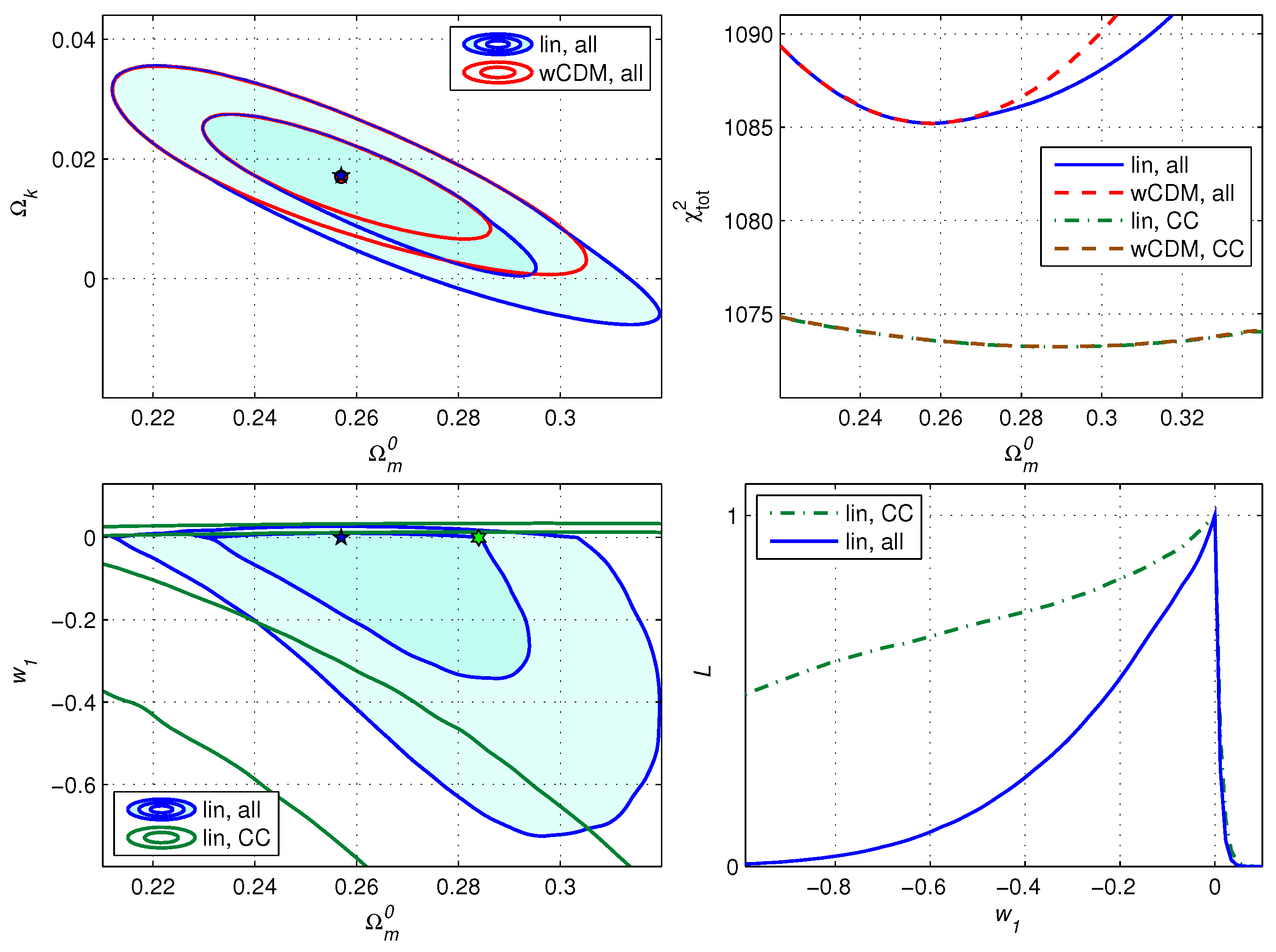
When we compare two models with different number $N_p$ of free parameters, we can expect that the model with larger $N_p$ achieves more success in minimizing ${\chi }_{\mathrm{tot}}^2$. However, some models are not successful in this sense. In particular, the linear model (3), (22) with $N_p=5$ parameters (28), with our set of observational data, yields the same minimal value $min{\chi }_{\mathrm{tot}}^2\simeq 1092.34$ (for CC + $H_{\mathrm{BAO}}$) as the wCDM model (24) with $N_p=4$. The reason is the following: the best fitted value $w_1$ for the linear model (3) is very close to zero ($w_1\simeq -0.0006$). In this case, the linear model works as the wCDM model (24) and yields the same $min{\chi }_{\mathrm{tot}}^2$.

Such a behavior of the model (3) is shown in Figure 1, where $1\sigma$ and $2\sigma$ filled contour plots in the left panels correspond to the full set of $H\left(z\right)$ data (here and below, “all” denotes CC + $H_{\mathrm{BAO}}$). The $1\sigma$, $2\sigma$ contours for the wCDM model (red lines) in the ${\Omega }_m^0-{\Omega }_k$ plane behave similarly and closely; positions of ${\chi }_{\mathrm{tot}}^2$ minima point (shown as the star and the circle) practically coincide.

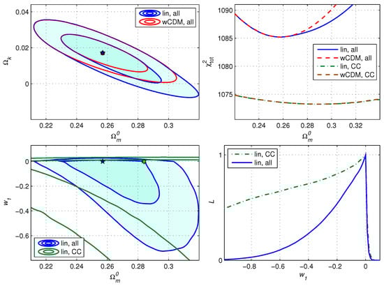
Figure 1. For the linear model (3), $1\sigma$, $2\sigma$ contour plots in the left panels (“all” means all $H\left(z\right)$ data); one-parameter distributions ${\chi }_{\mathrm{tot}}^2\left({\Omega }_m^0\right)$ and likelihood functions $\mathcal{L}\left(w_1\right)$ in the right panels are compared with the wCDM model. The stars and circles denote positions of ${\chi }_{\mathrm{tot}}^2$ minima points.

Here, the contours are drawn for ${\chi }^2$ functions minimized over all other parameters, in particular, for the linear model (3) in the top-left panel:

$${\chi }_{\mathrm{tot}}^2({\Omega }_m^0,{\Omega }_k)=\underset{H_0,w_0,w_1}{min}{\chi }_{\mathrm{tot}}^2.$$

(30)

A similar picture also takes place for only CC $H\left(z\right)$ data, where $min{\chi }_{\mathrm{tot}}^2\simeq 1074.73$ for both models. Equality of these minima for only CC and all $H\left(z\right)$ data is illustrated with one-parameter distributions ${\chi }_{\mathrm{tot}}^2\left({\Omega }_m^0\right)$ in the top-right panel. In one-parameter distributions, we also minimize over all other parameters.

In the ${\Omega }_m^0-w_1$ plane (the bottom-left panel) we see that for both models, minima of ${\chi }_{\mathrm{tot}}^2$ are achieved near $w_1=0$. It is also shown in the bottom-right panel, where the likelihood functions

$$\mathcal{L}\left(w_1\right)\sim exp\left[-{\chi }_{\mathrm{tot}}^2\left(w_1\right)/2\right]$$

(31)

are depicted for the linear model.

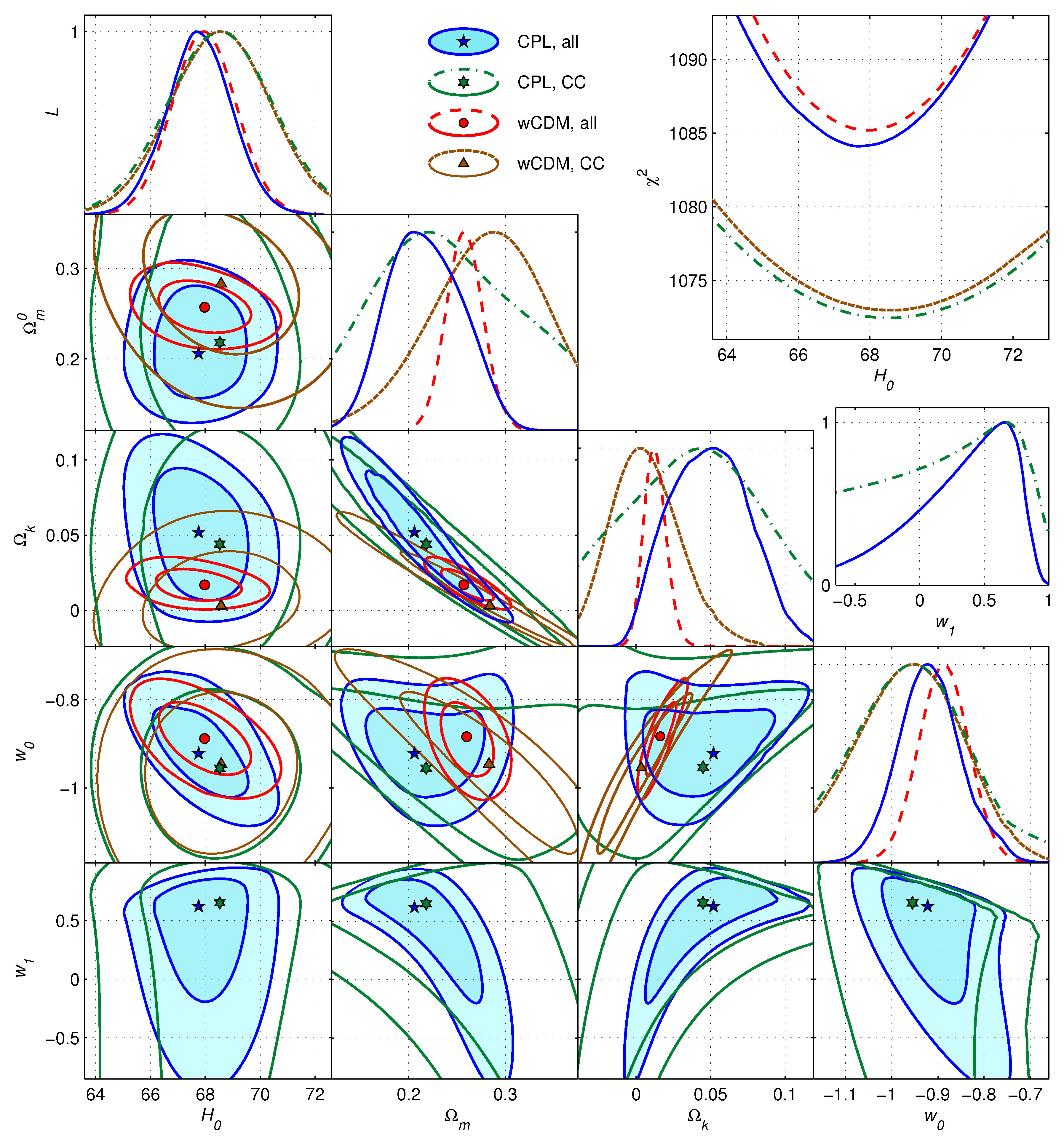
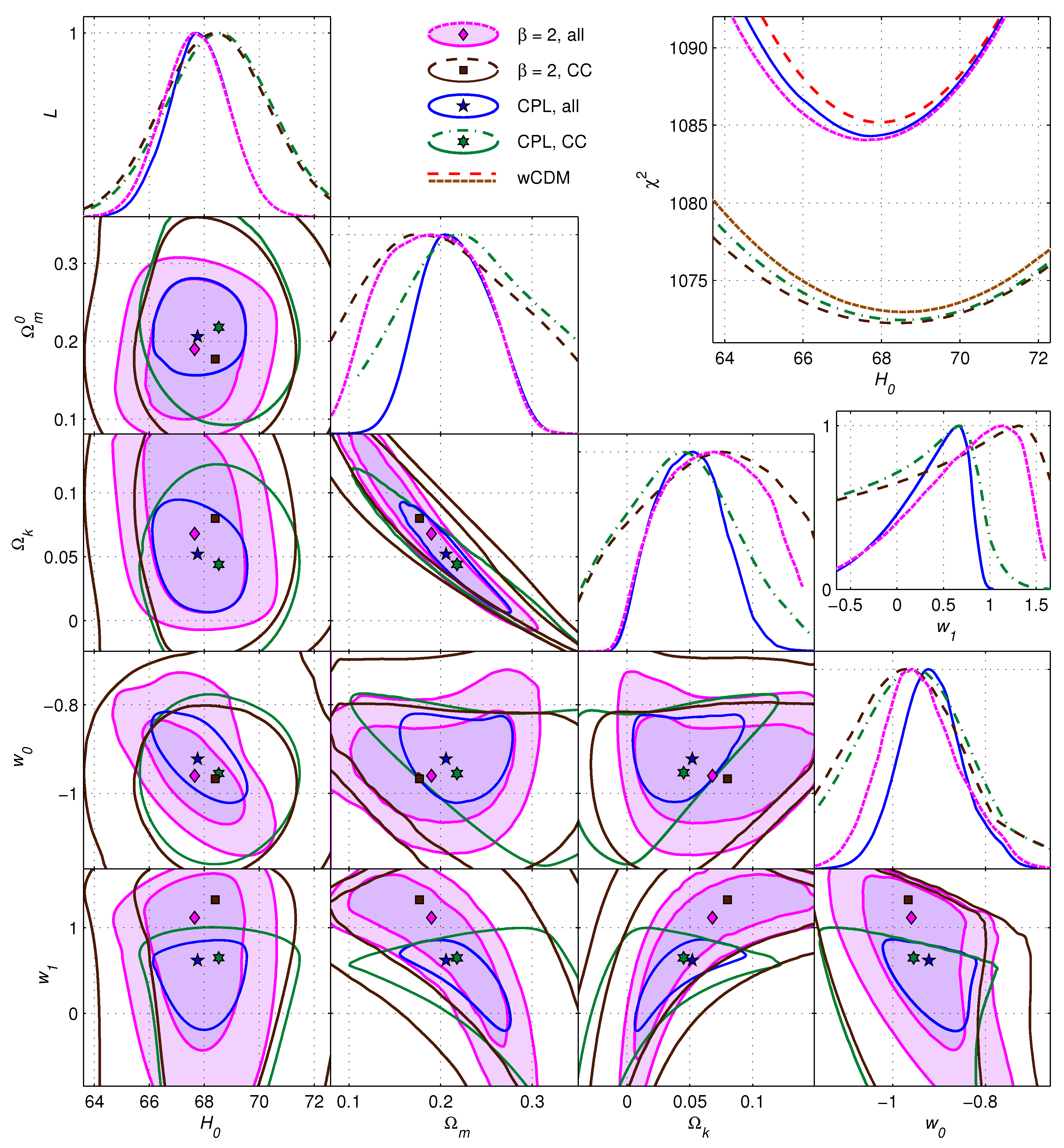
For the same observational data we can observe in Figure 2 more successful behavior of the Chevallier–Polarski–Linder (CPL) model (23) [23,24]. Here, $1\sigma$ and $2\sigma$ contours are drawn for ${\chi }_{\mathrm{tot}}^2({\theta }_i,{\theta }_j)$ of the type (30) in all planes of two parameters $({\theta }_i-{\theta }_j)$ in notation of Figure 1. We consider four cases: for two models (CPL and wCDM) we calculate ${\chi }_{\mathrm{tot}}^2$ for CC and all $H\left(z\right)$ data, positions of all ${\chi }_{\mathrm{tot}}^2$ minima points are shown. Naturally, in the panels with $w_1$, only the CPL model is presented.

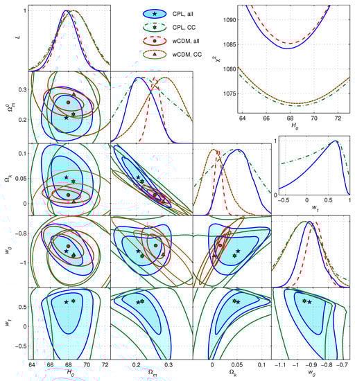
Figure 2. CPL model (23) in comparison with the wCDM model: $1\sigma$, $2\sigma$ contours, likelihoods $\mathcal{L}\left({\theta }_j\right)$, and one-parameter distributions ${\chi }_{\mathrm{tot}}^2\left(H_0\right)$.

The likelihood functions $\mathcal{L}\left({\theta }_i\right)$ of the type (31) are shown in Figure 2 for all five model parameters (28). They are used for estimating the best fits and $1\sigma$ errors for these parameters, summarized below in Table 2.

Table 2. The best fit values with $1\sigma$ estimates of model parameters and $min{\chi }_{\mathrm{tot}}^2$ for SNe Ia + CMB and CC or all $H\left(z\right)$ data for the models: $\beta =2$ (32), CPL (23), wCDM, and $\Lambda$CDM.

Model	Data	$min{\mathit{\chi }}_{\mathbf{tot}}^2/\mathit{d}.\mathit{o}.\mathit{f}$	${\mathit{H}}_0$	${\mathbf{\Omega }}_{\mathit{m}}^0$	${\mathbf{\Omega }}_{\mathit{k}}$	${\mathit{w}}_0\equiv \mathit{w}$	${\mathit{w}}_1$
$\beta =2$	CC	$1072.30/1079$	$68.{40}_{-1.91}^{+1.86}$	$0.{177}_{-0.072}^{+0.113}$	$0.{080}_{-0.076}^{+0.067}$	$-0.{967}_{-0.14}^{+0.12}$	$1.{33}_{-1.56}^{+0.42}$
CPL	CC	$1072.45/1079$	$68.{53}_{-1.88}^{+1.84}$	$0.{218}_{-0.074}^{+0.102}$	$0.{044}_{-0.059}^{+0.047}$	$-0.{955}_{-0.14}^{+0.14}$	$0.{65}_{-1.04}^{+0.25}$
$w$CDM	CC	$1072.97/1080$	$68.{58}_{-1.89}^{+1.85}$	$0.{283}_{-0.058}^{+0.055}$	$0.{003}_{-0.021}^{+0.024}$	$-0.{946}_{-0.14}^{+0.14}$	-
$\Lambda$CDM	CC	$1073.81/1081$	$68.{52}_{-1.94}^{+1.89}$	$0.{305}_{-0.029}^{+0.029}$	$0.{0052}_{-0.0018}^{+0.0018}$	$-1$	-
$\beta =2$	all	$1084.03/1115$	$67.{65}_{-1.26}^{+1.28}$	$0.{190}_{-0.072}^{+0.071}$	$0.{068}_{-0.053}^{+0.072}$	$-0.{96}_{-0.067}^{+0.087}$	$1.{12}_{-1.09}^{+0.40}$
CPL	all	$1084.28/1115$	$67.{76}_{-1.01}^{+1.15}$	$0.{206}_{-0.025}^{+0.054}$	$0.{052}_{-0.036}^{+0.027}$	$-0.{922}_{-0.06}^{+0.07}$	$0.{62}_{-0.52}^{+0.18}$
$w$CDM	all	$1085.19/1116$	$67.{98}_{-1.11}^{+1.11}$	$0.{257}_{-0.019}^{+0.019}$	$0.{017}_{-0.008}^{+0.008}$	$-0.{89}_{-0.05}^{+0.05}$	-
$\Lambda$CDM	all	$1089.42/1117$	$69.{02}_{-1.06}^{+1.04}$	$0.{272}_{-0.012}^{+0.013}$	$0.{004}_{-0.0017}^{+0.0017}$	$-1$	-

The CPL model achieves lower values of $min{\chi }_{\mathrm{tot}}^2$ in comparison with the wCDM and $\Lambda$CDM models. It can be seen in Table 2 and in the top-right panel of Figure 2, where one-parameter distributions ${\chi }_{\mathrm{tot}}^2\left(H_0\right)$ of these models are compared. The graphs ${\chi }_{\mathrm{tot}}^2\left(H_0\right)$ and the correspondent likelihoods $\mathcal{L}\left(H_0\right)$ in the top-left panel demonstrate that the best fitted values $H_0$ are very close for the wCDM and CPL models and differ more essentially when we compare CC and all $H\left(z\right)$ data.

The best fits of ${\Omega }_m^0$ depend stronger on the chosen model and vary from ${\Omega }_m^0\simeq 0.206$ for CPL, all $H\left(z\right)$ to ${\Omega }_m^0\simeq 0.289$ for wCDM, CC. The best fits of ${\Omega }_k$ behave similarly, but with the maximal estimate for CPL, all $H\left(z\right)$. The best CPL fits for $w_1$ are close to $0.66$ for both variants of $H\left(z\right)$ data. This value is far from zero; in other words, the CPL model with the considered observational data behaves differently to the wCDM model.

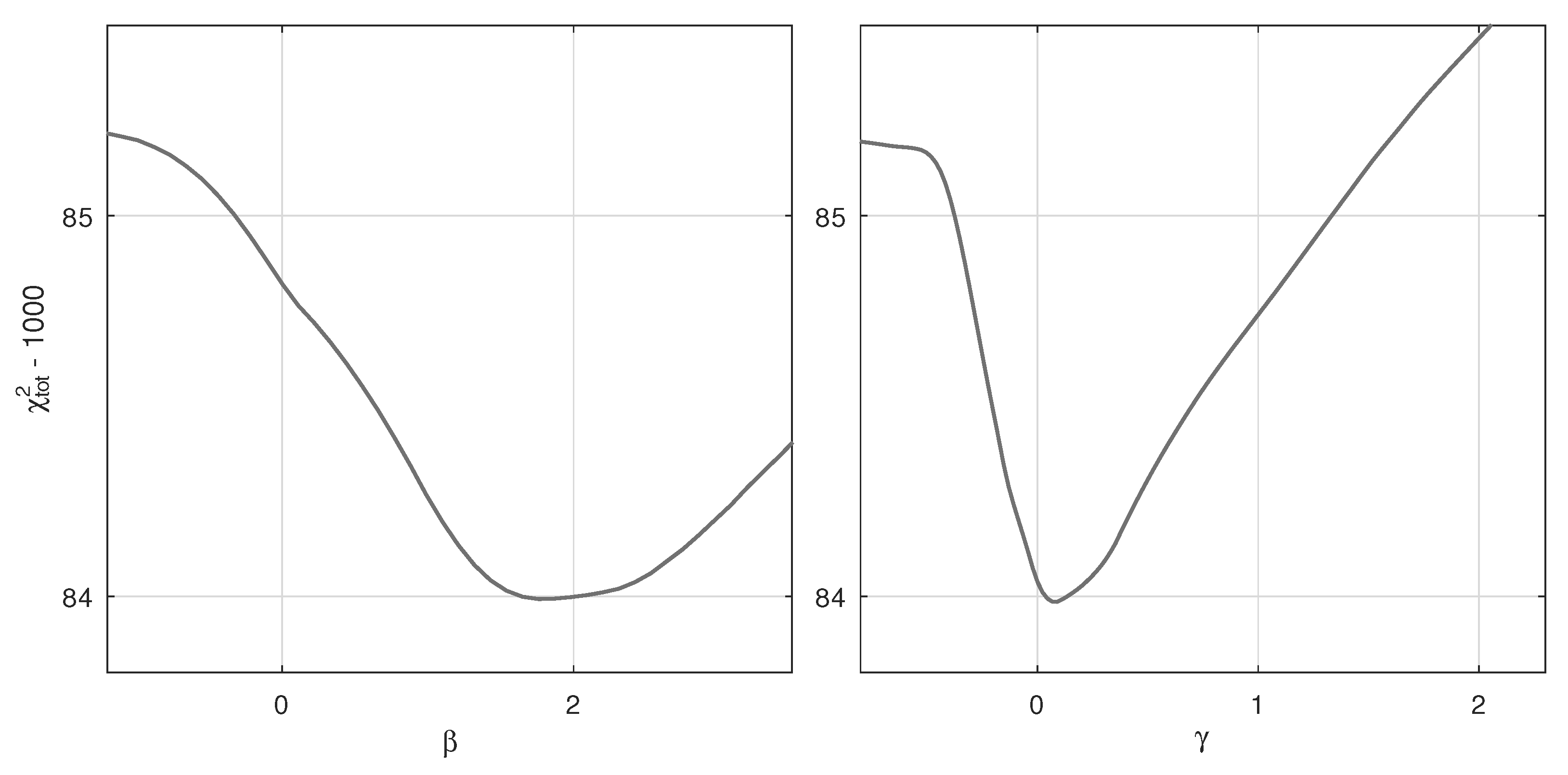
The CPL model achieves good results, but it is not the most successful scenario in the frameworks of the generalized model (7), (25). However, this generalized model has $N_p=7$ free parameters, including $\beta$ and $\gamma$ in addition to five parameters (28). This large number is the serious disadvantage of the generalized model (25) if we keep in mind informational criteria [19,20,21] and difficulties in calculations.

Following these reasons, we calculated the ${\chi }_{\mathrm{tot}}^2$ function (29) for the generalized model (18), (25) with all $H\left(z\right)$ data searching its minimum in the $\beta -\gamma$ plane. The results are presented in Figure 3 as one-parameter distributions ${\chi }_{\mathrm{tot}}^2\left(\beta \right)$ and ${\chi }_{\mathrm{tot}}^2\left(\gamma \right)$ (minimized over all other parameters).

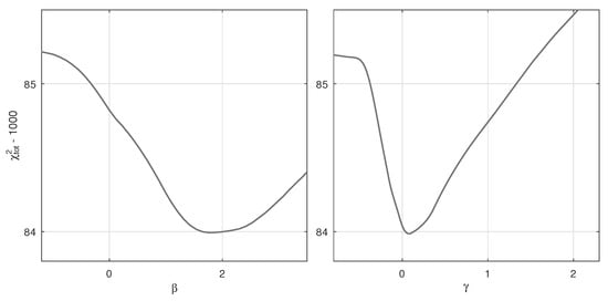
Figure 3. The generalized model (25) with all $H\left(z\right)$ data: one-parameter distributions for $\beta$ and $\gamma$.

We see in Figure 3 that the absolute minimum for the generalized model (25) $min{\chi }_{\mathrm{tot}}^2\simeq 1084.0$ is achieved near the point $\beta =2$, $\gamma =0$. One may conclude that the Barboza–Alcaniz–Zhu–Silva (BAZS) model [25] (corresponding to $\gamma =0$) with ${\Omega }_x\left(a\right)$ (21) and $\beta =2$ appeared to be the most successful for the considered observational data Ia + CMB + CC + $H_{\mathrm{BAO}}$. When we fix $\beta =2$, the BAZS model with

$$w=w_0+w_1(1-a^2)/2$$

(32)

will have five free model parameters (28). We investigate this model (denoted below as “$\beta =2$”) in detail; the results are presented in Table 2 and in Figure 4.

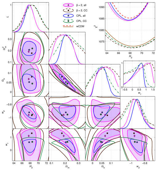
Figure 4. BAZS model $\beta =2$ (32) with $1\sigma$, $2\sigma$ contours in comparison with CPL model ($1\sigma$ contours), likelihoods $\mathcal{L}\left({\theta }_j\right)$, and one-parameter distributions ${\chi }_{\mathrm{tot}}^2\left(H_0\right)$.

Figure 4 illustrates the BAZS model with $\beta =2$ (32): $1\sigma$ and $2\sigma$ contour plots are shown for all $H\left(z\right)$ data (filled contours) and for only CC data. They are compared with the corresponding $1\sigma$ contours of the CPL model (shown also in Figure 2). One can compare the related one-parameter distributions ${\chi }_{\mathrm{tot}}^2\left(H_0\right)$ in the top-right panel and likelihood functions (31) $\mathcal{L}\left(H_0\right)$, $\mathcal{L}\left({\Omega }_m^0\right)$, $\mathcal{L}\left({\Omega }_k\right)$, etc.

Figure 4 and Table 2 demonstrate that the $\beta =2$ BAZS model (32) is more successful in minimizing ${\chi }_{\mathrm{tot}}^2$ if we compare it with the CPL model (and, naturally, with the wCDM and $\Lambda$CDM models). For only CC data and for all $H\left(z\right)$ data, the best fit values of ${\chi }_{\mathrm{tot}}^2$ for the $\beta =2$ model (32) are achieved at lower values of ${\Omega }_m^0$ (${\Omega }_m^0=0.{177}_{-0.072}^{+0.113}$ for CC and $0.{19}_{-0.072}^{+0.071}$ for all H data) and at larger values of ${\Omega }_k$ in comparison with CPL model. However, the best fit values of $H_0$ approximately coincide for all considered models; they depend on a chosen dataset: only CC data or all $H\left(z\right)$ data.

The best fitted values of $w_0$ are close for the $\beta =2$, CPL, and wCDM models in the CC case and slightly differ for all $H\left(z\right)$ data. The optimal values of $w_1$ are larger for the $\beta =2$ model ($w_1=1.{33}_{-1.56}^{+0.42}$ for CC and $1.{12}_{-1.09}^{+0.40}$ for all H data) if we compare with the CPL model; however, one should take into account the factor $\frac{1}{2}$ in EoS (32): $w=w_0+w_1(1-a^2)/2$.

To compare models with different number $N_p$ of free model parameters, we use here the Akaike information criterion [19,20,60]:

$$\mathrm{AIC}=min{\chi }_{tot}^2+2N_p.$$

(33)

This criterion emphasizes the advantage of models with small number of $N_p$. It can be seen in Table 3 for the mentioned models, where, for only CC $H\left(z\right)$ data, the minimal Akaike values (33) are achieved for the $\Lambda$CDM ($\mathrm{AIC}=1079.81$) and the wCDM ($\mathrm{AIC}=1080.97$) models. However, for all $H\left(z\right)$ data, the $\beta =2$ model (32) with $N_p=5$ parameters appeared to be more successful than $\Lambda$CDM not only in $min{\chi }_{\mathrm{tot}}^2\simeq 1084.03$, but also with Akaike information (33): $\mathrm{AIC}=1094.03$. The lowest $\mathrm{AIC}=1093.19$ is achieved here for the wCDM model.

Table 3. The best fits of $min{\chi }_{\mathrm{tot}}^2$, AIC, and $H_0$ for the models $\beta =2$ (32), CPL (23), wCDM, $\Lambda$CDM, and these models in the spatially flat case ($k=0$).

Model	Data	$min{\mathit{\chi }}_{\mathbf{tot}}^2$	AIC	${\mathit{H}}_0$	Flat Model	$min{\mathit{\chi }}_{\mathbf{tot}}^2/\mathit{d}.\mathit{o}.\mathit{f}$	AIC	${\mathit{H}}_0$
$\beta =2$	CC	$1072.30$	$1082.30$	$68.{40}_{-1.91}^{+1.86}$	flat $\beta =2$	$1072.99/1080$	$1080.99$	$68.{46}_{-1.81}^{+1.82}$
CPL	CC	$1072.45$	$1082.45$	$68.{53}_{-1.88}^{+1.84}$	flat CPL	$1072.98/1080$	$1080.98$	$68.{47}_{-1.80}^{+1.81}$
$w$CDM	CC	$1072.97$	$1080.97$	$68.{58}_{-1.89}^{+1.85}$	flat wCDM	$1073.01/1081$	$1079.01$	$68.{50}_{-1.79}^{+1.81}$
$\Lambda$CDM	CC	$1073.81$	$1079.81$	$68.{52}_{-1.94}^{+1.89}$	flat $\Lambda$CDM	$1073.93/1082$	$1077.93$	$69.{21}_{-1.91}^{+1.92}$
$\beta =2$	all	$1084.03$	$1094.03$	$67.{65}_{-1.26}^{+1.28}$	flat $\beta =2$	$1087.84/1116$	$1095.84$	$67.{81}_{-1.06}^{+1.12}$
CPL	all	$1084.28$	$1094.28$	$67.{76}_{-1.01}^{+1.15}$	flat CPL	$1087.56/1116$	$1095.56$	$67.{99}_{-1.16}^{+1.11}$
$w$CDM	all	$1085.19$	$1093.19$	$67.{98}_{-1.11}^{+1.11}$	flat wCDM	$1089.90/1117$	$1095.90$	$68.{16}_{-1.14}^{+1.12}$
$\Lambda$CDM	all	$1089.42$	$1095.42$	$69.{02}_{-1.06}^{+1.04}$	flat $\Lambda$CDM	$1089.96/1118$	$1093.96$	$68.{35}_{-0.55}^{+0.56}$

On the right side of the Table 3, we present the predictions of the same models on their flat case $k=0$ (${\Omega }_k=0$). In this case, the values $min{\chi }_{\mathrm{tot}}^2$ and AIC appeared to be larger, and the $\beta =2$ model (32) loses its advantage in comparison with CPL scenario for all $H\left(z\right)$ data.

5. Discussion

We considered different cosmological models with variable equations of state (EoS) for dark energy of the type (2) $p_x=w\left(a\right){\rho }_x$, more precisely, models with EoS (7),

$$w\left(a\right)=w_0+w_1\frac{1-a^{\beta }}{\beta }{a}^{\gamma },$$

generalizing the $\Lambda$CDM, wCDM, Chevallier–Polarski–Linder (CPL), and Barboza–Alcaniz–Zhu–Silva (BAZS) models [23,25]. These scenarios with nonzero spatial curvature and with ${\Omega }_k=0$ were confronted with observational data described in Section 2 and including SNe Ia, CMB data, and two classes of the Hubble parameter estimates $H\left(z\right)$: from cosmic chronometers (CC) and from line-of-sight baryonic acoustic oscillations ($H_{\mathrm{BAO}}$) data.

The results of our calculations for different models are presented in Table 2 and Table 3, including minima of ${\chi }_{\mathrm{tot}}^2$, Akaike information criterion (33), and the best fitted values with $1\sigma$ estimates of model parameters. We also investigated the linear model (3), (22) with $N_p=5$ parameters (28), however it appeared to be unsuccessful because it achieved the best fitted value of ${\chi }_{\mathrm{tot}}^2$ at $w_1$ very close to zero (see Figure 1). In other words, the linear model (22) with the considered observational data was reduced to the wCDM model with only $N_p=4$ parameters, but both models have the same $min{\chi }_{\mathrm{tot}}^2$.

Unlike the linear model (22) CPL scenario (4), (23) with the same $N_p=5$ parameters (28) appeared to be more successful, in particular, for all $H\left(z\right)$ data, the CPL model yields $min{\chi }_{\mathrm{tot}}^2\simeq 1084.28$ in comparison with $1085.19$ for the wCDM and $1089.42$ for the $\Lambda$CDM models. In this case, the best fitted value $w_1\simeq 0.62$ is far from zero, so CPL is not reduced to the wCDM model.

We should remember that a large number $N_p$ of free model parameters is a drawback of any model, and when we use, in Table 3, the Akaike information criterion (33), the wCDM model with $\mathrm{AIC}=1093.19$ will have the advantage over CPL with $\mathrm{AIC}=1094.28$ (and more essential advantage over the $\Lambda$CDM model with $1095.42$). If we consider the generalized model (7), (25) with $N_p=7$ and additional parameters $\beta$ and $\gamma$, the Akaike expression (33) becomes too large and the model looks worse in comparison with others.

However, our analysis and Figure 3 showed that the minimum $min{\chi }_{\mathrm{tot}}^2\simeq 1084.03$ of the generalized model (25) may be achieved if we fix $\beta =2$, $\gamma =0$; the resulting model “$\beta =2$” (32) has the same $N_p=5$ parameters (28) and absolutely minimal $min{\chi }_{\mathrm{tot}}^2$ for all $H\left(z\right)$ data (its $\mathrm{AIC}=1094.03$ is behind only the wCDM AIC). The behavior of one-parameter distributions ${\chi }_{\mathrm{tot}}^2\left(H_0\right)$ and their minima for all models with all $H\left(z\right)$ data are shown in Figure 5.

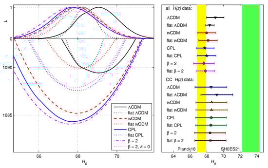
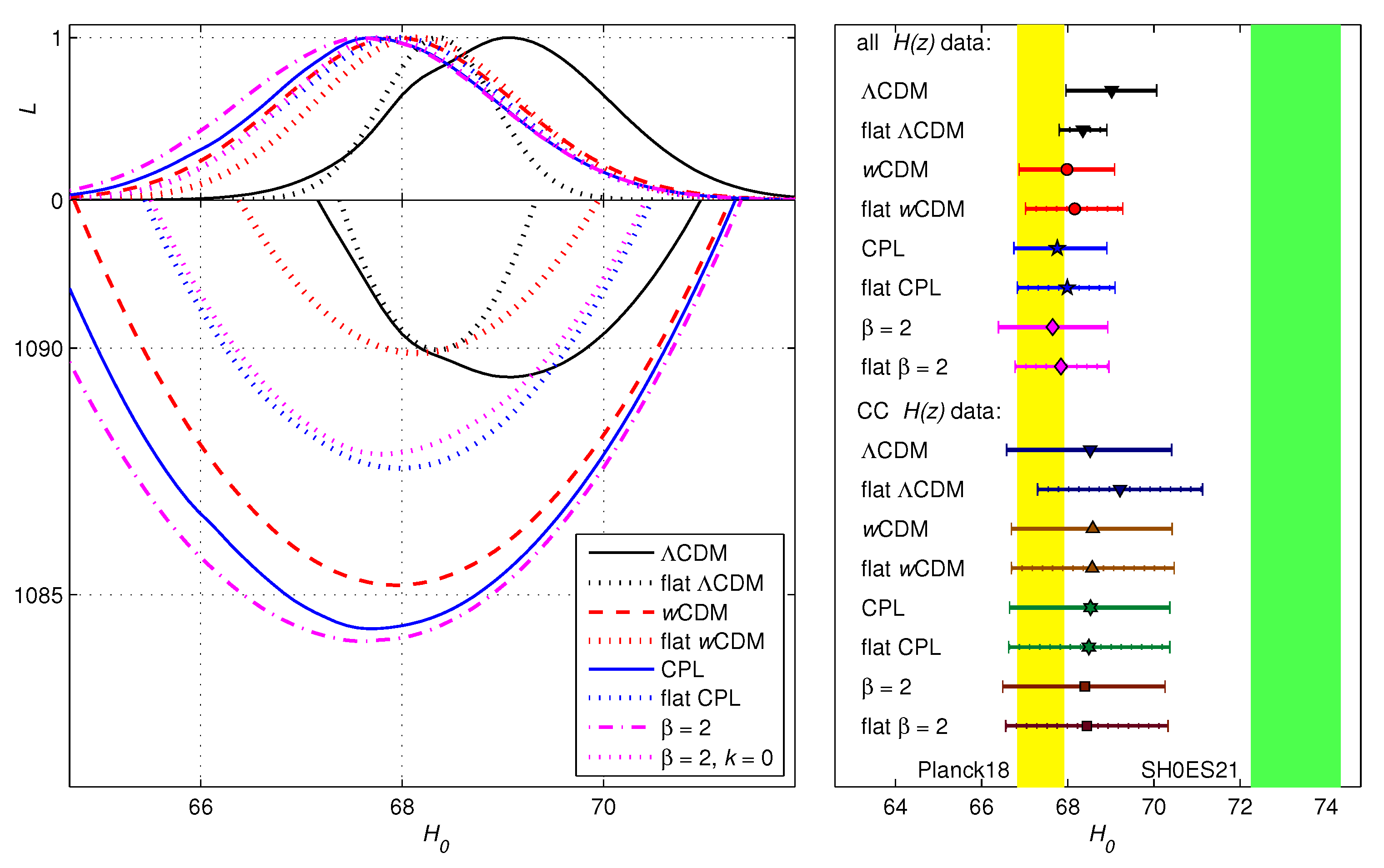
Figure 5. One-parameter distributions ${\chi }_{\mathrm{tot}}^2\left(H_0\right)$ and likelihood functions for models with all $H\left(z\right)$ data (the flat cases $k=0$ are shown with dotted lines); $H_0$ estimates in the right panel are drawn as whisker plots.

As mentioned above, if we use only CC $H\left(z\right)$ data, we observe smaller differences between minima of ${\chi }_{\mathrm{tot}}^2$ for the considered models in Table 2. In this case, the Akaike criterion (33) gives advantage to the $\Lambda$CDM model with minimal $N_p$.

Table 2 and Figure 2 and Figure 4 demonstrate that the success of the CPL scenario is achieved at lower (best fitted) values of ${\Omega }_m^0$ and at larger values of ${\Omega }_k$, if we compare these results with the wCDM model. This tendency is strengthened for the $\beta =2$ model (32). It looks natural, because the CPL model (23) is the particular case of the BAZS model (21) with $\beta =1$.

One can see in Table 2 and Table 3 and Figure 2, Figure 4, and Figure 5 that the best fitted values of the Hubble parameter $H_0$ are very close for models wCDM, CPL, and $\beta =2$ in general and spatially flat cases. However, the predictions of these models diverge with that of the $\Lambda$CDM model for all $H\left(z\right)$ data. The last result is illustrated in Figure 5; it becomes more clear if we look at Figure 2, keeping in mind that the $\Lambda$CDM model is the particular case of the wCDM model when $w=-1$. One should add the observed difference between $H_0$ estimates of all models when we compare CC and all $H\left(z\right)$ data.

In the left panels of Figure 5 we draw one-parameter distributions ${\chi }_{\mathrm{tot}}^2\left(H_0\right)$ and likelihood functions (31) $\mathcal{L}\left(H_0\right)$ for the considered models with all $H\left(z\right)$ data to clarify their best fits of $H_0$. For the considered four models we demonstrate here the results for the flat cases $k=0$ (${\Omega }_k=0$) as dotted lines.

One can see that in the flat case $k=0$, the mentioned models yield appreciably larger minima $min{\chi }_{\mathrm{tot}}^2$, but the best fitted values of $H_0$ change unessentially for the wCDM, CPL, and $\beta =2$ models. For the flat $\Lambda$CDM model, the graph ${\chi }_{\mathrm{tot}}^2\left(H_0\right)$ is inscribed between the correspondent graphs of the general $\Lambda$CDM and flat wCDM models; hence, the $H_0$ estimate for the flat $\Lambda$CDM model lies between two estimates of the mentioned scenarios.

All $H_0$ predictions of the wCDM, CPL, and $\beta =2$ models with all $H\left(z\right)$ data fit the Planck 2018 estimation of the Hubble constant [2] (see Figure 5), but they are far from the SH0ES 2021 estimation [4]. All $H_0$ predictions with CC $H\left(z\right)$ data are very close for the four considered models and their flat variants: they are larger but overlap the Planck 2018 value; however, they cannot describe the tension with the SH0ES data.

We can see from Table 3 that the best values of AIC (33) for all $H\left(z\right)$ data demonstrate the wCDM and $\beta =2$ (32) models, but for CC $H\left(z\right)$ data, the best AIC has the flat $\Lambda$CDM model.

References

- Ade, P.A.; Aghanim, N.; Arnaud, M.; Ashdown, M.; Aumont, J.; Baccigalupi, C.; Banday, A.J.; Barreiro, R.B.; Bartlett, J.G.; Bartolo, N.; et al. Planck 2015 results. XIII. Cosmological parameters. Astron. Astrophys. 2016, 594, A13. [Google Scholar]
- Aghanim, N.; Akrami, Y.; Ashdown, M.; Aumont, J.; Baccigalupi, C.; Ballardini, M.; Banday, A.J.; Barreiro, R.B.; Bartolo, N.; Basak, S.; et al. Planck 2018 results. VI. Cosmological parameters. Astron. Astrophys. 2020, 641, A6. [Google Scholar]
- Riess, A.G.; Casertano, S.; Yuan, W.; Bowers, J.B.; Macri, L.; Zinn, J.C.; Scolnic, D. Cosmic Distances Calibrated to 1% Precision with Gaia EDR3 Parallaxes and Hubble Space Telescope Photometry of 75 Milky Way Cepheids Confirm Tension with ΛCDM. Astrophys. J. Lett. 2021, 908, L6. [Google Scholar] [CrossRef]
- Riess, A.G.; Yuan, W.; Macri, L.M.; Scolnic, D. A Comprehensive Measurement of the Local Value of the Hubble Constant with 1 km/s/Mpc Uncertainty from the Hubble Space Telescope and the SH0ES Team. Astrophys. J. Lett. 2021, 908, L6. [Google Scholar]
- Riess, A.G.; Casertano, S.; Yuan, W.; Macri, L.M.; Scolnic, D. Large Magellanic Cloud Cepheid Standards Provide a 1% Foundation for the Determination of the Hubble Constant and Stronger Evidence for Physics Beyond LambdaCDM. Astrophys J. 2019, 876, 85. [Google Scholar] [CrossRef]
- Bamba, K.; Capozziello, S.; Nojiri, S.; Odintsov, S.D. Dark energy cosmology: The equivalent description via different theoretical models and cosmography tests. Astrophys. Space Sci. 2012, 342, 155–228. [Google Scholar] [CrossRef] [Green Version]
- Nojiri, S.; Odintsov, S.D. Unified cosmic history in modified gravity: From F(R) theory to Lorentz non-invariant models. Phys. Rept. 2011, 505, 59–144. [Google Scholar] [CrossRef] [Green Version]
- Odintsov, S.D.; Oikonomou, V.K. Modified Gravity Theories on a Nutshell: Inflation, Bounce and Late-time Evolution. Phys. Rept. 2017, 692, 1–104. [Google Scholar]
- Di Valentino, E.; Anchordoqui, L.A.; Ali-Haimoud, Y.; Amendola, L.; Arendse, N.; Asgari, M.; Ballardini, M.; Battistelli, E.; Benetti, M.; Birrer, S. Cosmology Intertwined II: The Hubble Constant Tension. Astropart. Phys. 2021, 131, 102605. [Google Scholar] [CrossRef]
- Di Valentino, E.; Mena, O.; Pan, S.; Visinelli, L.; Yang, W.; Melchiorri, A.; Mota, D.F.; Riess, A.G.; Silk, J. In the Realm of the Hubble tension—A Review of Solutions. Class. Quantum Grav. 2021, 38, 153001. [Google Scholar] [CrossRef]
- Kumar, S.; Nunes, R.C. Probing the interaction between dark matter and dark energy in the presence of massive neutrinos. Phys. Rev. D 2016, 94, 123511. [Google Scholar] [CrossRef] [Green Version]
- Kumar, S.; Nunes, R.C. Echo of interactions in the dark sector. Phys. Rev. D 2017, 96, 103511. [Google Scholar] [CrossRef] [Green Version]
- Pan, S.; Yang, W.; Di Valentino, E.; Saridakis, E.N.; Chakraborty, S. Interacting scenarios with dynamical dark energy: Observational constraints and alleviation of the H0 tension. Phys. Rev. D 2019, 100, 103520. [Google Scholar] [CrossRef] [Green Version]
- Di Valentino, E.; Melchiorri, A.; Mena, O.; Vagnozzi, S. Interacting dark energy in the early 2020s: A promising solution to the H0 and cosmic shear tensions. Phys. Dark Univ. 2020, 30, 100666. [Google Scholar] [CrossRef]
- Pan, S.; Sharov, G.S. A model with interaction of dark components and recent observational data. Mon. Not. R. Astron. Soc. 2017, 472, 4736. [Google Scholar] [CrossRef]
- Pan, S.; Sharov, G.S.; Yang, W. Field theoretic interpretations of interacting dark energy scenarios and recent observations. Phys. Rev. D 2020, 101, 103533. [Google Scholar] [CrossRef]
- Odintsov, S.D.; Saez-Gomez, D.; Sharov, G.S. Testing the equation of state for viscous dark energy. Phys. Rev. D 2020, 101, 044010. [Google Scholar] [CrossRef] [Green Version]
- Odintsov, S.D.; Saez-Gomez, D.; Sharov, G.S. Is exponential gravity a viable description for the whole cosmological history? Eur. Phys. J. C 2017, 77, 862. [Google Scholar] [CrossRef] [Green Version]
- Odintsov, S.D.; Saez-Gomez, D.; Sharov, G.S. Testing logarithmic corrections to R2-exponential gravity by observational data. Phys. Rev. D 2019, 99, 024003. [Google Scholar] [CrossRef] [Green Version]
- Nojiri, S.; Odintsov, S.D.; Saez-Gomez, D.; Sharov, G.S. Modelling and testing the equation of state for (Early) dark energy. Phys. Dark Univ. 2021, 32, 100837. [Google Scholar] [CrossRef]
- Odintsov, S.D.; Saez-Gomez, D.; Sharov, G.S. Analyzing the H0 tension in F(R) gravity models. Nucl. Phys. B 2021, 966, 115377. [Google Scholar] [CrossRef]
- Cooray, A.R.; Huterer, D. Gravitational Lensing as a Probe of Quintessence. Astrophys. J. 1999, 513, L95–L98. [Google Scholar] [CrossRef] [Green Version]
- Chevallier, M.; Polarski, D. Accelerating Universes with Scaling Dark Matter. Int. J. Mod. Phys. D 2001, 10, 213–224. [Google Scholar] [CrossRef] [Green Version]
- Linder, E.V. Exploring the expansion history of the universe. Phys. Rev. Lett. 2003, 90, 091301. [Google Scholar] [CrossRef] [PubMed] [Green Version]
- Barboza, E.M.; Alcaniz, J.S.; Zhu, Z.-H.; Silva, R. A generalized equation of state for dark energy. Phys. Rev. D 2009, 80, 043521. [Google Scholar] [CrossRef]
- Scolnic, D.M.; Jones, D.O.; Rest, A.; Pan, Y.C.; Chornock, R.; Foley, R.J.; Huber, M.E.; Kessler, R.; Narayan, G.; Riess, A.G.; et al. The Complete Light-curve Sample of Spectroscopically Confirmed Type Ia Supernovae from Pan-STARRS1 and Cosmological Constraints from The Combined Pantheon Sample. Astrophys. J. 2018, 859, 101. [Google Scholar] [CrossRef]
- Chen, L.; Huang, Q.-G.; Wang, K. Distance priors from Planck final release. J. Cosmol. Astropart. Phys. 2019, 1902, 028. [Google Scholar] [CrossRef] [Green Version]
- Nesseris, S.; Perivolaropoulos, L. Comparison of the legacy and gold SN Ia dataset constraints on dark energy models. Phys. Rev. D 2005, 72, 123519. [Google Scholar] [CrossRef] [Green Version]
- Efstathiou, G. To H0 or not to H0? Mon. Not. R. Astron. Soc. 2021, 505, 3866–3872. [Google Scholar] [CrossRef]
- Camarena, D.; Marra, V. On the use of the local prior on the absolute magnitude of Type Ia supernovae in cosmological inference. Mon. Not. R. Astron. Soc. 2021, 504, 5164–5171. [Google Scholar] [CrossRef]
- Nunes, R.C.; Di Valentino, E. Dark sector interaction and the supernova absolute magnitude tension. Phys. Rev. D 2021, 104, 063529. [Google Scholar] [CrossRef]
- Hu, W.; Sugiyama, N. Small Scale Cosmological Perturbations: An Analytic Approach. Astrophys. J. 1996, 471, 542–570. [Google Scholar] [CrossRef] [Green Version]
- Sharov, G.S.; Sinyakov, E.S. Cosmological models, observational data and tension in Hubble constant. Math. Model. Geom. 2020, 8, 1–20. [Google Scholar] [CrossRef]
- Simon, J.; Verde, L.; Jimenez, R. Constraints on the redshift dependence of the dark energy potential. Phys. Rev. D. 2005, 71, 123001. [Google Scholar] [CrossRef] [Green Version]
- Stern, D.; Jimenez, R.; Verde, L.; Kamionkowski, M.; Stanford, S.A. Cosmic Chronometers: Constraining the Equation of State of Dark Energy. I: H(z) Measurements. JCAP 2010, 1002, 008. [Google Scholar] [CrossRef] [Green Version]
- Moresco, M.; Cimatti, A.; Jimenez, R.; Pozzetti, L.; Zamorani, G.; Bolzonella, M.; Dunlop, J.; Lamareille, F.; Mignoli, M.; Pearce, H.; et al. Improved constraints on the expansion rate of the Universe up to z∼1.1 from the spectroscopic evolution of cosmic chronometers. JCAP 2012, 1208, 006. [Google Scholar] [CrossRef] [Green Version]
- Zhang, C.; Zhang, H.; Yuan, S.; Zhang, T.-J.; Sun, Y.-C. Four New Observational H(z) Data From Luminous Red Galaxies Sloan Digital Sky Survey Data Release Seven. Res. Astron. Astrophys. 2014, 14, 1221. [Google Scholar] [CrossRef] [Green Version]
- Moresco, M. Raising the bar: New constraints on the Hubble parameter with cosmic chronometers at z∼2. Mon. Not. R. Astron. Soc. 2015, 450, L16. [Google Scholar] [CrossRef] [Green Version]
- Moresco, M.; Pozzetti, L.; Cimatti, A.; Jimenez, R.; Maraston, C.; Verde, L.; Thomas, D.; Citro, A.; Tojeiro, R.; Wilkinson, D. A 6% measurement of the Hubble parameter at z∼0.45: Direct evidence of the epoch of cosmic re-acceleration. JCAP 2016, 1605, 014. [Google Scholar] [CrossRef] [Green Version]
- Ratsimbazafy, A.L.; Loubser, S.I.; Crawford, S.M.; Cress, C.M.; Bassett, B.A.; Nichol, R.C.; Väisänen, P. Age-dating Luminous Red Galaxies observed with the Southern African Large Telescope. Mon. Not. R. Astron. Soc. 2017, 467, 3239. [Google Scholar] [CrossRef] [Green Version]
- Borghi, N.; Moresco, M.; Cimatti, A. Towards a Better Understanding of Cosmic Chronometers: A new measurement of H(z) at z=0.7. arXiv 2021, arXiv:2110.04304. [Google Scholar] [CrossRef]
- Moresco, M.; Jimenez, R.; Verde, L.; Cimatti, A.; Lucia Pozzetti, L. Setting the Stage for Cosmic Chronometers. II. Impact of Stellar Population Synthesis Models Systematics and Full Covariance Matrix. Astrophys. J. 2020, 898, 82. [Google Scholar] [CrossRef]
- Moresco, M.; Amati, L.; Amendola, L.; Birrer, S.; Blakeslee, J.P.; Cantiello, M.; Cimatti, A.; Darling, J.; Valle, M.D.; Fishbach, M.; et al. Unveiling the Universe with Emerging Cosmological Probes. Astrophys. J. 2020, 898, 82. [Google Scholar] [CrossRef]
- Gaztañaga, E.; Cabre, A.; Hui, L. Clustering of Luminous Red Galaxies IV: Baryon Acoustic Peak in the Line-of-Sight Direction and a Direct Measurement H(z). Mon. Not. Roy. Astron. Soc. 2009, 399, 1663. [Google Scholar] [CrossRef] [Green Version]
- Blake, C.; Brough, S.; Colless, M.; Contreras, C.; Couch, W.; Croom, S.; Croton, D.; Davis, T.M.; Drinkwater, M.J.; Forster, K.; et al. The WiggleZ Dark Energy Survey: Joint measurements of the expansion and growth history at z<1. Mon. Not. R. Astron. Soc. 2012, 425, 405. [Google Scholar]
- Chuang, C.-H.; Wang, Y. Modeling the Anisotropic Two-Point Galaxy Correlation Function on Small Scales and Improved Measurements of H(z), DA(z), and f(z)σ8(z) from the Sloan Digital Sky Survey DR7 Luminous Red Galaxies. Mon. Not. R. Astron. Soc. 2013, 435, 255. [Google Scholar] [CrossRef] [Green Version]
- Chuang, C.-H.; Prada, F.; Cuesta, A.J.; Eisenstein, D.J.; Kazin, E.; Padmanabhan, N.; Sánchez, A.G.; Xu, X.; Beutler, F.; Manera, M.; et al. The clustering of galaxies in the SDSS-III Baryon Oscillation Spectroscopic Survey: Single-probe measurements and the strong power of f(z)σ8(z) on constraining dark energy. Mon. Not. R. Astron. Soc. 2013, 433, 3559. [Google Scholar] [CrossRef]
- Busca, N.G.; Delubac, T.; Rich, J.; Bailey, S.; Font-Ribera, A.; Kirkby, D.; Le Goff, J.-M.; Pieri, M.M.; Slosar, A.; Aubourg, E.; et al. Baryon Acoustic Oscillations in the Lyα forest of BOSS quasars. Astron. Astrophys. 2013, 552, A96. [Google Scholar] [CrossRef] [Green Version]
- Oka, A.; Saito, S.; Nishimichi, T.; Taruya, A.; Yamamoto, K. Simultaneous constraints on the growth of structure and cosmic expansion from the multipole power spectra of the SDSS DR7 LRG sample. Mon. Not. R. Astron. Soc. 2014, 439, 2515–2530. [Google Scholar] [CrossRef]
- Font-Ribera, A.; Kirkby, D.; Busca, N.; Miralda-Escudé, J.; Ross, N.P.; Slosar, A.; Rich, J.; Aubourg, E.; Bailey, S.; Bhardwaj, V.; et al. Quasar-Lyman α Forest Cross-Correlation from BOSS DR11: Baryon Acoustic Oscillations. J. Cosmol. Astropart. Phys. 2014, 2014, 027. [Google Scholar] [CrossRef]
- Delubac, T.; Bautista, J.E.; Busca, N.G.; Rich, J.; Kirkby, D.; Bailey, S.; Font-Ribera, A.; Slosar, A.; Lee, K.-G.; Pieri, M.M.; et al. Baryon Acoustic Oscillations in the Lyα forest of BOSS DR11 quasars. Astron. Astrophys. 2015, 574, A59. [Google Scholar] [CrossRef] [Green Version]
- Anderson, L.; Aubourg, E.; Bailey, S.; Beutler, F.; Bhardwaj, V.; Blanton, M.; Bolton, A.S.; Brinkmann, J.; Brownstein, J.R.; Burden, A.; et al. The clustering of galaxies in the SDSS-III Baryon Oscillation Spectroscopic Survey: Baryon Acoustic Oscillations in the Data Release 10 and 11 Galaxy Samples. Mon. Not. R. Astron. Soc. 2014, 441, 24. [Google Scholar] [CrossRef] [Green Version]
- Wang, Y.; Zhao, G.-B.; Chuang, C.-H.; Ross, A.J.; Percival, W.J.; Gil-Martín, H.; Cuesta, A.J.; Kitaura, F.-S.; Rodriguez-Torres, S.; Brownstein, J.R.; et al. The clustering of galaxies in the completed SDSS-III Baryon Oscillation Spectroscopic Survey: Tomographic BAO analysis of DR12 combined sample in configuration space. Mon. Not. R. Astron. Soc. 2017, 469, 3762. [Google Scholar] [CrossRef]
- Alam, S.; Ata, M.; Bailey, S.; Beutler, F.; Bizyaev, D.; Blazek, J.A.; Bolton, A.S.; Brownstein, J.R.; Burden, A.; Chuang, C.-H.; et al. The clustering of galaxies in the completed SDSS-III Baryon Oscillation Spectroscopic Survey: Cosmological analysis of the DR12 galaxy sample. Mon. Not. R. Astron. Soc. 2017, 470, 2617. [Google Scholar] [CrossRef] [Green Version]
- Bautista, J.E.; Busca, N.G.; Guy, J.; Rich, J.; Blomqvist, M.; Bourboux, H.M.; Pieri, M.M.; Font-Ribera, A.; Bailey, S.; Delubac, T.; et al. Measurement of baryon acoustic oscillation correlations at z=2.3 with SDSS DR12 Lyα-Forests. Astron. Astrophys. 2017, 603, A12. [Google Scholar] [CrossRef] [Green Version]
- Bourboux, H.; Le Goff, J.-M.; Blomqvist, M.; Busca, N.G.; Guy, J.; Rich, J.; Yèche, C.; Bautista, J.E.; Burtin, E.; Dawson, K.S.; et al. Baryon acoustic oscillations from the complete SDSS-III Lyα-quasar cross-correlation function at z=2.4. Astron. Astrophys. 2017, 608, A130. [Google Scholar] [CrossRef] [Green Version]
- Zhu, F.; Padmanabhan, N.; Ross, A.J.; White, M.; Percival, W.J.; Ruggeri, R.; Zhao, G.-B.; Wang, D.; Mueller, E.-M.; Burtin, E.; et al. The clustering of the SDSS-IV extended Baryon Oscillation Spectroscopic Survey DR14 quasar sample: Measuring the anisotropic Baryon Acoustic Oscillations with redshift weights. Mon. Not. R. Astron. Soc. 2018, 480, 1096. [Google Scholar] [CrossRef] [Green Version]
- Zhao, G.-B.; Wang, Y.; Saito, S.; Gil-Martín, H.; Percival, W.J.; Wang, D.; Chuang, C.-H.; Ruggeri, R.; Mueller, E.-M.; Zhu, F.; et al. The clustering of the SDSS-IV extended Baryon Oscillation Spectroscopic Survey DR14 quasar sample: Tomographic measurement of cosmic structure growth and expansion rate based on optimal redshift weights. Mon. Not. R. Astron. Soc. 2019, 482, 3497. [Google Scholar] [CrossRef] [Green Version]
- Ade, P.A.; Aghanim, N.; Armitage-Caplan, C.; Arnaud, M.; Ashdown, M.; Atrio-Barandela, F.; Aumont, J.; Baccigalupi, C.; Banday, A.J.; Barreiro, R.B.; et al. Planck 2013 results. XVI. Cosmological parameters. Astron. Astrophys. 2014, 571, A16. [Google Scholar]
- Akaike, H. A New Look at the Statistical Model Identification. IEEE Trans. Autom. Control 1974, 19, 716–723. [Google Scholar] [CrossRef]
Publisher’s Note: MDPI stays neutral with regard to jurisdictional claims in published maps and institutional affiliations. |
© 2022 by the authors. Licensee MDPI, Basel, Switzerland. This article is an open access article distributed under the terms and conditions of the Creative Commons Attribution (CC BY) license (https://creativecommons.org/licenses/by/4.0/).