Abstract
We study the gamma-ray burst (GRB) afterglow light curves produced by an off-axis jet in a stratified circumburst medium and summarize the temporal indices of the coasting phase, the deceleration phase, the Newtonian phase, and the deep Newtonian phase for various viewing angles and power-law indices of medium density. Generally, the afterglow light curves of off-axis GRBs in the homogeneous interstellar medium have a steep rise arising due to jet deceleration. In the stratified medium, the flux rises is more shallow but peaks earlier for the same viewing angle due to faster deceleration of the jet running into the denser stratified medium, compared with the case of the interstellar medium (ISM). Observations of off-axis bursts will possibly increase over the coming years due to the arrival of the multi-messenger era and the forthcoming surveys in multiple bands. The temporal indices of off-axis afterglows derived in the paper will provide a reference for comparison with the observations and can diagnose the circumburst environment. The numerical code calculating the afterglow light curve also can be used to fit the multi-wavelength light curves.
1. Introduction
In the gamma-ray burst (GRB) standard model, afterglows are produced by the interaction between a fireball shell and the homogeneous interstellar medium (ISM) [1,2]. A pair of shocks, forward shock and reverse shock, will be developed when the shell begins to decelerate considerably after sweeping up enough circumburst medium (CBM). The forward shock starts to experience a self-similar expansion subsequently [3]. Electrons in the shocked medium are accelerated. Assuming a power-law distribution of the electrons and considering the dynamic evolution of the shock, one can find the muti-segment broken power-law radiation spectrum and light curve [4], which is called the standard afterglow model. The power-law decay of light curves predicted by the standard afterglow model has been widely tested and confirmed by abundant observations. However, the afterglow light curves in some bursts displayed a marked achromatic steepening break lately, suggesting that at least some GRB fireballs are possibly not spherical but collimated jets [5,6]. The extremely high isotropic gamma-ray energy in some bursts also can be explained in the jet model. During the ultra-relativistic phase, the light curves of the afterglow from a jet are not different from those from a spherical fireball due to the relativistic beaming effect if the line of sight (LOS) is within the jet. Thus the standard afterglow model still applies in this phase until the jet edge is seen or the lateral expansion becomes significant. After that, the light curve will become steeper [7,8].
A natural consequence of the jet model is the presence of off-axis bursts. Some GRBs have spectral peaks of tens of keV or less, much lower than those of typical bursts which were believed to arise from off-axis jets with viewing angles larger than jet half opening angles e.g., [9,10] or from off-axis structured jets (e.g., [11]). It is also possible that if the observer is off-axis, we could miss GRBs but observe their late afterglows when the beaming effect becomes weak due to jet deceleration. This is the so-called “orphan afterglow”, whose detectability has been extensively investigated [7,12,13,14,15,16,17,18,19,20]. The detection of an orphan afterglow will be essential evidence of the GRB jet model. However, until now, no definite orphan afterglow detection has been reported (however, see [21] for some candidates). Off-axis afterglow light curves have been studied for various jet models [13,20,22,23,24,25]. Generally, the light curves have a rapid rise initially and then peak when the jet Lorentz factor decreases down to , where is the jet half opening angle. The rising amplitude depends on the viewing angle if the CBM is homogeneous.
Another factor that can considerably affect the afterglow light curve is the circumburst environment. Observations have supported the model that long GRBs are produced in the collapse of a massive star [26,27,28]. Thus, the CBM density is expected to be inhomogeneous and decrease in radius due to the wind from the progenitor star. For a free wind with constant mass-loss rate and wind speed, the number density of CBM scales as with the radius R of the afterglow shock [29,30,31,32]. The power-law slope of density can deviate from two due to variable mass-loss rate and wind speed, which are poorly known. Short bursts usually happen outside of their host galaxy due to a long migration with a large kick speed before the merger of a compact binary, where the CBM density transits from the ISM to the intergalactic medium (IGM). Their CBM is usually homogeneous and is more rarefied than that of long bursts [33]. However, it is not excluded that some short bursts happen in a density fluctuation region, which may have an ununiform density profile, approximately described by a power-law profile (stratified medium). Indeed, there are individual bursts, whose light curves can be explained by the wind medium model e.g., [34]. Some temporal properties of the afterglow’s forward and reverse shocks in the stratified medium have been investigated [35,36]. Compared with the ISM case, in the stratified medium, the density is large in small radii. Thus the jet deceleration is fast at the beginning and will gradually become slower due to the decreasing medium density with the increase in the radius. This will lead to different light curves from those in the standard model.
Recently, a well-known short GRB 170817A was found, which was the first GRB associated with a gravitational-wave event [37] and marked the dawn of multi-messenger astronomy. Compared with other GRBs, the afterglow of the burst has a multi-wavelength rise with a power-law slope of ∼0.8, lasting for as long as ∼160 days, which has never been found in other bursts. The isotropic energy of the burst is 3–4 orders of magnitude lower than the conventional short bursts. These unconventional properties strongly suggest that this burst arises from a structured jet seen off-axis [38,39,40,41,42,43,44,45]. Thus this detection of the burst opened the era of the observation of off-axis bursts.
Stimulated by the long rise of GRB 170817A, here we systematically study the off-axis afterglow light curves from a uniform GRB jet in the stratified medium (although this burst may not be the case), paying more attention to the analytical scalings and numerical calculation of the light curves. The scalings and light curves could serve as a reference to the observations of off-axis bursts in the future. The paper is organized as follows. In Section 2, we analytically derive the off-axis light curves in the stratified medium in various regimes. In Section 3, we numerically calculate the light curves using a dynamic model to test the analytical results. The summary and discussion are provided in the last section. Table 1 lists the acronyms used in the paper.

Table 1.
Alphabetically ordered list of the acronyms used in this paper.
2. The Analytical Light Curves from an Off-Axis Jet in the Stratified Medium
Consider a relativistic outflow at a radius R from the burst source collimated into an initial opening angle running into the CBM. The CBM can be the ISM or the wind-like medium whose density can be described by a simple power-law profile e.g., [30,31]. More generally, regardless of the exact mechanism, one can consider a power-law stratified number density as
where is the density at an initial radius of . A forward shock and a reverse shock will form. Here we only consider the forward shock. When the shock sweeps up enough CBM whose mass is equal to ( is the initial Lorentz factor of the ejecta) of the rest mass of the ejecta, it begins to decelerate significantly and enters a self-similar expansion, corresponding to the onset of the GRB afterglow [46,47]. Before the deceleration, the Lorentz factor of the shock is nearly constant, corresponding to the so-called coasting phase.
2.1. Coasting Phase
With the evolution of the shock, its radius will increase with the burst source time . Here T is the observer time, is the angle between the speed of a fluid element within the jet and the viewing line, and c is the light speed. Note that in the analytical consideration, we neglect the redshift z. In the coasting phase, the shock speed is a constant. The observed time is thus . For the off-axis case, the emission of the jet mainly comes from the nearest angular region of the jet from the viewing line unless the viewing line is very close to the jet edge. Thus, as an approximation, we only consider the nearest point of the jet from the viewing line. Given the viewing angle , for and , one can find
In the following analytical consideration, we focus our attention on the off-axis case where is easily satisfied before significant lateral expansion (we neglect the lateral expansion in the rising phase of the light curves in the analytical estimation) unless the viewing line is very close to the edge of the jet.
We can find and . The total electron number in the shocked ejecta is . The observed synchrotron typical frequency and the cooling frequency are and , respectively. Here and with being the electron mass and being the electron energy fraction. is defined as the “effective” Doppler factor, which is the Doppler effect of the fluid element at . The magnetic field behind the shock is [48], is the magnetic field energy fraction of the internal energy and is the proton mass. Note that primed quantities are measured in the shock co-moving frame and that following the often-used notation, the magnetic field, energy equipartition parameters, electron energies, and electron distribution are unprimed, although they are measured in the co-moving frame. The observed flux peak is , where is the synchrotron peak spectral power. In the coasting phase, we can find that
In low-frequency bands (e.g., the radio band), synchrotron self-absorption (SSA) has to be considered. Two regimes, including fast cooling () and slow cooling (), will be involved successively due to the evolution of and . For typical parameters, the afterglow light curves are generally in the two regimes of and . The SSA frequency scales as [49,50]
Hence, following the synchrotron spectra [4], the light curves can be described by
and
If the observed band in early time falls in the spectral segment of or , for the ISM case, we have or , respectively, while for the wind case (s = 2), the light curves scale as or (p = 2.3) for or , respectively. These are consistent with previous results (e.g., [51,52]). For a general density profile , the light curve slopes fall in between the two cases. See Table 2 for the slopes with 2 and .
Table 2.
Temporal indexes from an off-axis jet in the coasting phase for .
2.2. Deceleration Phase
In the decelerating phase, considering the adiabatic case, the isotropic equivalent energy of the shocked fluid is [3], implying . The shock radius is thus
The Lorentz factor of the shocked fluid scales as
Thus, we obtain
The SSA frequency in the regimes of and scales as [49,50]
Thus the light curves in the deceleration phase are
and
The analytical temporal indexes for with a typical value of for the fast and slow cooling cases in the deceleration phase are shown in Table 3 and Table 4, respectively. Note that in Table 3 and Table 4, we include the regimes of and . In the dense CBM, it is also possible that the SSA frequency is larger than max(, ). We derive the light curve indexes for these cases in the Appendix A. We can find if the observed frequency is in and , the light curve index is ∼4.1. If , the rising index is ∼0.7 for . These are roughly consistent with [52]. Given the rising index of ∼0.8 for light curves of GRB 170817A, the density index would be if the burst happened in the stratified medium.
Table 3.
Temporal indexes from an off-axis jet for the fast-cooling regime in the deceleration phase (p = 2.3).
Table 4.
Temporal indexes from an off-axis jet for the slow-cooling regime in the deceleration phase (p = 2.3).
2.3. Late Afterglow
This preceding derivation of light curves does not include the sideways expansion, which is not significant at early times. However, it will become significant when the jet slows down to [7,8]. The jet will rapidly start an approximately spherical expansion, and . The light curves for various viewing angles will have a common decline as [8] until the expansion enters the Newtonian phase when the rest of the swept-up mass-energy is equal to the shock energy. For the ISM and the wind-like medium, the light curves in this phase have been investigated [53,54,55,56,57]. For more general CBM, using the so-called Sedov–Taylor solution e.g., [58], one can find the scalings: , , , , and . Thus the light curves scale as
Considering the density profiles of , one can find the flux scales as and for and , respectively, which are consistent with previous analytical results (e.g., [54,56]). The scalings within square brackets are for the wind medium. For later times, the shock will enter the deep Newtonian phase with , below which the synchrotron approximation becomes invalid. One can only consider the electrons with energy and neglect the lower-energy electrons. Using the total electron number emitting synchrotron photons and ([59], or see the similar treatment in [60,61]), we can find
The indexes for the sideways expanding phase (when the sideways expansion becomes significant), the Newtonian phase, and the deep Newtonian phase are displayed in Table 5. For and , , which is in agreement with previous results (e.g., [60]). One can find the light curves for gradually transit from ∼2.3 [2.3] to ∼−1.4 [−1.9] and then to ∼−1.1 [−1.2] in the ISM wind-like medium, i.e., the light curves gradually become shallow.
Table 5.
Temporal indexes from an off-axis jet at late times for p = 2.3.
3. The Numerical Calculation of Afterglow Light Curves
3.1. Dynamic Evolution of the Afterglow Jet
The analytical estimates give the light curve slopes but neglect some details, including the geometry shape of the jet, sideways expansion of the jet, etc. To derive more precise light curves, we should appeal to numerical calculations of the dynamic evolution and radiation. The dynamic evolution of a jet has been extensively investigated e.g., [7,8,55,57,62,63]. In these studies, the sideways expansion is a crucial factor but remains an open question. Recent numerical and analytical studies have found that sideways expansion is not as fast as predicted in the analytical model (e.g., [7,57]). However, Ref. [64] reached the opposite conclusion. It appears that if the initial opening angle is quite small, sideway expansion approaches the prediction of the analytical model, while if it is large, the sideway expansion is slow [63]. Regardless of the debate, we use the recent dynamic evolution model of [44], in which the evolution equation of the jet opening angle is
where is the dimensionless velocities, and is the dimensionless lateral expansion speed in the burst source frame. In the dynamic equations in [44], the finding that the “conical” spreading is more accurate than the “trumpet” model [62] is also taken into account (see Ryan et al. [44] for more details on the dynamic equations). The dynamic equations appear to obtain similar light curves to those of the multi-dimensional hydrodynamic simulation.
3.2. Flux Calculation
We will numerically calculate the afterglow light curve in this section. Consider a jet with the half opening angle of . The observed flux for a given observed time T can be given by [20,65]
where is the shocked shell width within which the radiation is effectively produced, and is the luminosity distance. The observed time T is the function of , R, and and can be given by
For a homogeneous jet, the flux can be reduced as
where
is the Doppler factor for a jet element. is the co-moving emissivity, i.e.,
where is the maximum Lorentz factor of the injected electrons and is the electron charge. is the pitch angle () averaged synchrotron spectral power, written as [66]
and is the Larmor frequency. is the modified Bessel function [67]. is the electron distribution (the electron number per unit energy Lorentz factor per unit volume). For the fast cooling case (), the distribution is
where is the co-moving electron density. While for the slow cooling () case, it is
We have taken SSA into account in the calculation. is the SSA optical depth and is the SSA coefficient and it is given by [67]
3.3. Code Verification
We have developed a Fortran code to solve the dynamic equations derived by [44] and calculate the light curve. The fourth-order Runge–Kutta algorithm is used to solve R(t), u(t), and on a fixed logarithmically spaced grid of t [68]. For a given observed time T, the observed flux is calculated by numerically integrating over the equal arrival time surface defined by Equation (19). The Steffensen iteration method is used to find the integral interval faster than the usual iteration method. The Gaussian integration is used [68]. The integral interval is split into multiple segments to improve the integral precision. To test the code, we compare the calculated light curves with those calculated by afterglowpy (see Ryan et al. [44]), shown in Figure 1. On the whole, the agreement of the two sets of light curves is good, especially in the early and late afterglow phases. In the intermediate phase, our results are somewhat higher than that derived by afterglowpy. In detail, our results are somewhat higher than those derived by afterglowpy, especially in the optical and radio bands (top panel of Figure 1). This is due to the fact that we consider the pitch angle as an averaged synchrotron spectrum, which will lead to a slight change in the synchrotron peak frequency and spectral power. If we use the analytical synchrotron spectrum as in [44], the agreement of the two codes is fairly good (see the bottom panel in Figure 1). There is also a slight difference in the intermediate phase, which can be attributed to the different numerical methods or numerical precision. It appears that our results approach those of Boxfit (see Figure 2 in Ryan et al. [44]).
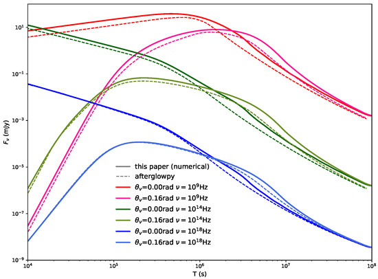
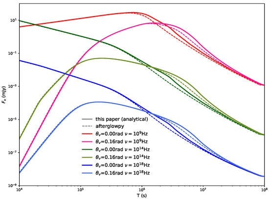
Figure 1.
Comparison of light curves calculated by afterglowpy [44] and our code for a homogeneous jet. The parameters in both codes are: rad, erg, n = cm3, p = 2.2, = 0.1, = 0.01, cm, and z = 0.028. In the top and bottom panels, the light curves are derived with the numerical and analytical synchrotron spectra, respectively. The latter spectrum is also adopted in Ryan et al. [44].
3.4. Comparison with the Analytical Results
In order to compare with the analytical results, we calculate the following light curve adopting the following typical parameters: , , , , , erg, , and cm. The initial Lorentz factor is used. The CBM number density for various s is set to be the typical value of the ISM at the on-axis jet break radius , where the lateral expansion becomes significant, i.e., [22,69]. The jet break radius can be given from , i.e., . Then the values of for others can be derived by . The values of are , , , and for s=0.5, 1, 1.5, and 2, respectively.
Figure 2 and Figure 3 depict the light curves and their slopes for the typical parameters with and , respectively. To show how the light curves are formed, the evolution of the Lorentz factor and the three typical frequencies are also included in the figures. For , we can find at an early time, that the X-ray bands ( keV) are in the regime of or in the coasting phase and thus the slope is ∼2 (see Table 2). Then the X-ray gradually goes into the regime of of the deceleration phase, so the X-ray light curve transits from 2 to 4.6 (see Table 3). The optical ( Hz) flux rises with the slope of in the regime of of the coasting phase and then transits from to with and then to , like the X-ray. The radio () band is in the same regime as the optical band. Thus the radio flux rises with a slope of and then with . Later, the jet edge is visible, whose light curve index is not easy to derive. After the whole jet is visible, the jet roughly declines with a slope of ∼. At a later time, the jet goes into the Newtonian phase. The flux in the three bands all decline with a slope of ∼ (see Table 5). We can find in the early and late times the analytical slopes are roughly consistent in the numerical results. At the intermediate time, the beaming effect becomes weaker with the deceleration of the jet, and the visible region increases. The jet’s sideways expansion also becomes significant. The total effect on the light curves is not easy to describe with the analytical method. The case of is similar (see Figure 3).
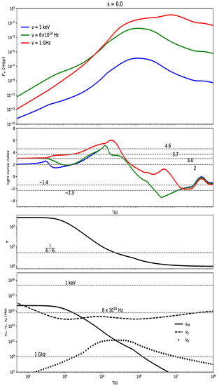
Figure 2.
Evolution of the flux (), the light curve index, the Lorentz factor of the jet (), and the typical frequencies of , , and with the observer time for the medium slope of . The typical parameters are used (see Section 3.4). In the second panel, the horizon dashed lines mark the analytical light curve indexes. In the third panel, the horizon dashed line shows the position where the Lorentz factor slows down to ). In the fourth panel, the horizontal dashed lines mark the three frequencies of 1 keV, 6 Hz, and 1 GHz.
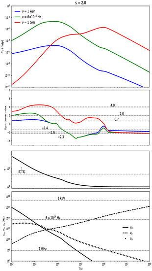
Figure 3.
Same as Figure 2 but for .
3.5. Typical Off-Axis Light Curves in a Stratified Medium
We numerically calculated multi-band light curves, including radio (1 GHz), optical ( Hz), and X-ray (1 keV) bands with different density slopes and various viewing angles of , as shown in Figure 4, Figure 5 and Figure 6. We find that the light curves exhibit a variety of shapes depending on different viewing angles and medium-density profiles. The resulting light curves are similar to those of [22] except in the radio band. We find the SSA is quite significant for the medium profile with large s, which is not taken into consideration in [22]. We also note that, compared with the ISM case, the off-axis light curves in the stratified medium depict a more shallow rise whose rising slopes depend on the medium density slope, but the light curves peak earlier than in the ISM case. This is because the density of the stratified medium is denser than the ISM, especially at small radii, leading to the faster deceleration of the jet and the jet edge being visible earlier. The rising duration depends on the viewing angle. The large viewing angle arises as a long rising phase but with a lower peak flux, which is harder to detect.
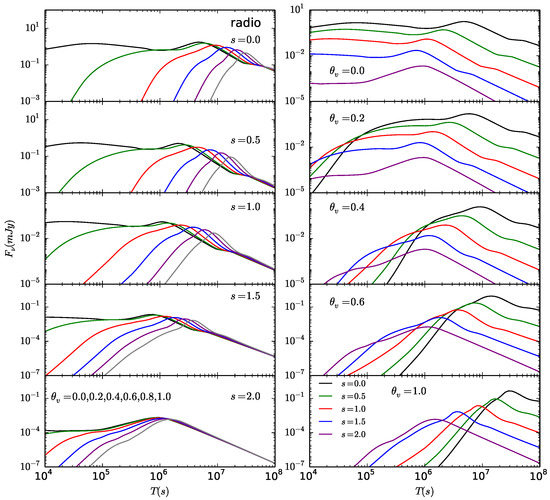
Figure 4.
Numerical light curves in the radio band (1 GHz). The left panels: light curves for various slopes of CBM number density with different viewing angles of . The right panels: light curves for various viewing angles of with different slopes of CBM number density.
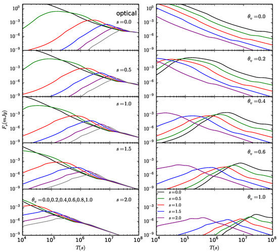
Figure 5.
Same as Figure 4 but for the optical band ( Hz).
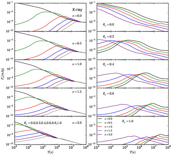
Figure 6.
Same as Figure 4 but for the X-ray band (1 keV).
4. Summary and Discussion
In this paper, we derive the analytical off-axis light curves of GRB afterglows in the stratified external medium with a power-law profile and summarize the scalings of off-axis light curves from the afterglow onset to the deep Newtonian phase (see Table 2, Table 3, Table 4 and Table 5), except for the intermediate phase. These light curve scalings can serve as a helpful tool for afterglow observers to quickly identify the spectral regime and the medium density profile from their data. Then we present the numerical afterglow light curves in radio, optical, and X-ray bands for a wide range of viewing angles in the stratified external medium. These results verify the analytical scalings for early and late afterglow. The numerical calculation code of the light curves can also be used to fit the multi-wavelength light curves fitting.
Previous works have derived the light curve scalings of off-axis afterglows for ISM (s = 0) and steady wind (s = 2) (e.g., [51,52,53,54,56,60]). However, some fittings to afterglow data have found that the medium slopes are not 0 or 2 but have other values (e.g., Yi et al. [35], Liang et al. [70], Kouveliotou et al. [71]), suggesting the CBM is not ISM and the preburst wind speed and/or mass-loss rate are not constant, otherwise leading to a medium slope of . In this paper, we generalize the scalings for arbitrary power-law circumburst density profiles, including ISM and wind. This can qualitatively diagnose the circumburst density profile from afterglow observations. Further, the observed afterglow light curves can be fitted with theoretical light curves by numerical methods, which will be used to determine the circumburst environment quantitatively.
A prominent feature of the off-axis afterglow light curves in the stratified medium is their shallow rising. If the viewing angle is large, we will observe a long and shallow rising. It is widely known that the off-axis structured jet also can give rise to a long and shallow rising in the light curve, which is used to explain the light curve of GRB 170817A (e.g., Lazzati et al. [42], Ghirlanda et al. [72], Kasliwal et al. [73]). This rising mechanism is due to the combined effect of the jet deceleration and the increase in the energy density and Lorentz factor at larger angles from the LOS (but closer to the jet core) where the emission is observable at later times. The two risings can be similar, but the underlying models may be distinguished from the late light curves. In the Newtonian or deep Newtonian phases, the decay indices of the light curves depend on the power-law slopes (s) of CBM and the power-law indexes of the electron distribution (see Table 5). The power-law indexes (p) of the electron distribution can be obtained by the observed spectrum. Thus, we can derive the power-law slopes of CBM, which, in turn, can be used to test whether the rising phase is entirely due to the stratified medium or not since the rising phase can also depend on the s and p in most cases. If a burst from a structured jet happens in the stratified CBM, both rising mechanisms are responsible for the light curves. The late afterglow light curve is crucial to diagnosing the jet structure and the density profile of CBM. A challenge is the late afterglow could be too faint to be well detected unless it happens close to us. The upcoming X-ray, optical, or radio survey (e.g., Einstein Probe, Yuan et al. [74]; the Large Synoptic Survey Telescope, LSST Science Collaboration et al. [75]) will possibly detect more off-axis bursts and provide more information on the GRB circumburst environment for us.
Author Contributions
Conceptualization, X.-H.Z.; Data curation, K.-F.C.; Investigation, X.-H.Z. and K.-F.C.; Validation, K.-F.C.; Visualization, K.-F.C.; Writing—original draft, X.-H.Z.; Writing—review & editing, X.-H.Z. and K.-F.C. All authors have read and agreed to the published version of the manuscript.
Funding
This work was supported by the National Science Foundation of China (Nos. U1831135), the Guangxi Natural Science Foundation (GKAD22035205), and the Scientific Research Project of Guangxi Minzu University (2021KJQD03).
Institutional Review Board Statement
Not applicable.
Informed Consent Statement
Not applicable.
Data Availability Statement
Data available on reasonable request to the authors.
Acknowledgments
We thank C. Y. Yang, Z. Li, and B. B. Zhang for useful discussions.
Conflicts of Interest
The authors declare no conflict of interest.
Appendix A. Off-Axis Afterglow Light Curves for νm < νa < νc, νc < νa < νm, νa > max(νc, νm)
In the afterglow phase, the SSA frequency is usually smaller than and in the normal ISM, whose light curves have been given in the context. However, is possibly larger than the two characteristic frequencies in a dense environment (e.g., the stellar wind environment). We thus include the cases in the appendix. For fast cooling, the SSA frequency scales as (e.g., [50])
while for slow cooling, we have
The light curves in the fast cooling case can be described by
and
depending on the ordering of and the other two characteristic frequencies, while in the slow cooling case, they go as
and
The situation could be more complex. For , electrons will be piled up at the energy corresponding to and thermalized [76,77]. This will considerably change the light curves. We will consider this case in the future.
References
- Katz, J.I. Low-Frequency Spectra of Gamma-Ray Bursts. Astrophys. J. 1994, 432, L107–L109. [Google Scholar] [CrossRef]
- Mészáros, P.; Rees, M.J. Optical and Long-Wavelength Afterglow from Gamma-Ray Bursts. Astrophys. J. 1997, 476, 232–237. [Google Scholar] [CrossRef]
- Blandford, R.D.; McKee, C.F. Fluid dynamics of relativistic blast waves. Phys. Fluids 1976, 19, 1130–1138. [Google Scholar] [CrossRef]
- Sari, R.; Piran, T.; Narayan, R. Spectra and Light Curves of Gamma-Ray Burst Afterglows. Astrophys. J. 1998, 497, L17–L20. [Google Scholar] [CrossRef]
- Harrison, F.A.; Bloom, J.S.; Frail, D.A.; Sari, R.; Kulkarni, S.R.; Djorgovski, S.G.; Axelrod, T.; Mould, J.; Schmidt, B.P.; Wieringa, M.H.; et al. Optical and Radio Observations of the Afterglow from GRB 990510: Evidence for a Jet. Astrophys. J. 1999, 523, L121–L124. [Google Scholar] [CrossRef]
- Kulkarni, S.R.; Djorgovski, S.G.; Odewahn, S.C.; Bloom, J.S.; Gal, R.R.; Koresko, C.D.; Harrison, F.A.; Lubin, L.M.; Armus, L.; Sari, R.; et al. The afterglow, redshift and extreme energetics of the γ-ray burst of 23 January 1999. Nature 1999, 398, 389–394. [Google Scholar] [CrossRef]
- Rhoads, J.E. The Dynamics and Light Curves of Beamed Gamma-Ray Burst Afterglows. Astrophys. J. 1999, 525, 737–749. [Google Scholar] [CrossRef]
- Sari, R.; Piran, T.; Halpern, J.P. Jets in Gamma-Ray Bursts. Astrophys. J. 1999, 519, L17–L20. [Google Scholar] [CrossRef]
- Heise, J.; Zand, J.I.; Kippen, R.M.; Woods, P.M. Gamma-Ray Bursts in the Afterglow Era; Costa, E., Frontera, F., Hjorth, J., Eds.; Springer: Berlin/Heidelberg, Germany, 2001; p. 16. [Google Scholar]
- Yamazaki, R.; Ioka, K.; Nakamura, T. X-ray Flashes from Off-Axis Gamma-Ray Bursts. Astrophys. J. 2002, 571, L31–L35. [Google Scholar] [CrossRef]
- Zhang, B.; Dai, X.; Lloyd-Ronning, N.M.; Mészáros, P. Quasi-universal Gaussian Jets: A Unified Picture for Gamma-Ray Bursts and X-Ray Flashes. Astrophys. J. 2004, 601, L119–L122. [Google Scholar] [CrossRef]
- Ghirlanda, G.; Burlon, D.; Ghisellini, G.; Salvaterra, R.; Bernardini, M.G.; Campana, S.; Covino, S.; D’Avanzo, P.; D’Elia, V.; Melandri, A.; et al. GRB Orphan Afterglows in Present and Future Radio Transient Surveys. Publ. Astron. Soc. Aust. 2014, 31, 22. [Google Scholar] [CrossRef][Green Version]
- Granot, J.; Panaitescu, A.; Kumar, P.; Woosley, S.E. Off-Axis Afterglow Emission from Jetted Gamma-Ray Bursts. Astrophys. J. 2002, 570, L61–L64. [Google Scholar] [CrossRef]
- Huang, Y.F.; Dai, Z.G.; Lu, T. Failed gamma-ray bursts and orphan afterglows. Mon. Not. R. Astron. Soc. 2002, 332, 735–740. [Google Scholar] [CrossRef]
- Lamb, G.P.; Tanaka, M.; Kobayashi, S. Transient survey rates for orphan afterglows from compact merger jets. Mon. Not. R. Astron. Soc. 2018, 476, 4435–4441. [Google Scholar] [CrossRef]
- Levinson, A.; Ofek, E.O.; Waxman, E.; Gal-Yam, A. Orphan Gamma-Ray Burst Radio Afterglows: Candidates and Constraints on Beaming. Astrophys. J. 2002, 576, 923–931. [Google Scholar] [CrossRef]
- Nakar, E.; Piran, T.; Granot, J. The Detectability of Orphan Afterglows. Astrophys. J. 2002, 579, 699–705. [Google Scholar] [CrossRef]
- Totani, T.; Panaitescu, A. Orphan Afterglows of Collimated Gamma-Ray Bursts: Rate Predictions and Prospects for Detection. Astrophys. J. 2002, 576, 120–134. [Google Scholar] [CrossRef]
- Zou, Y.C.; Wu, X.F.; Dai, Z.G. Estimation of the detectability of optical orphan afterglows. Astron. Astrophys. 2007, 461, 115–119. [Google Scholar] [CrossRef]
- van Eerten, H.; Zhang, W.; MacFadyen, A. Off-axis Gamma-ray Burst Afterglow Modeling Based on a Two-dimensional Axisymmetric Hydrodynamics Simulation. Astrophys. J. 2010, 722, 235–247. [Google Scholar] [CrossRef]
- Ho, A.Y.Q.; Perley, D.A.; Yao, Y.; Svinkin, D.; Postigo, A.d.; Perley, R.A.; Kann, D.A.; Burns, E.; Andreoni, I.; Bellm, E.C.; et al. Cosmological Fast Optical Transients with the Zwicky Transient Facility: A Search for Dirty Fireballs. arXiv 2022, arXiv:2201.12366. [Google Scholar] [CrossRef]
- Granot, J.; De Colle, F.; Ramirez-Ruiz, E. Off-axis afterglow light curves and images from 2D hydrodynamic simulations of double-sided GRB jets in a stratified external medium. Mon. Not. R. Astron. Soc. 2018, 481, 2711–2720. [Google Scholar] [CrossRef]
- Moderski, R.; Sikora, M.; Bulik, T. On Beaming Effects in Afterglow Light Curves. Astrophys. J. 2000, 529, 151–156. [Google Scholar] [CrossRef]
- Rossi, E.; Lazzati, D.; Rees, M.J. Afterglow light curves, viewing angle and the jet structure of r-ray bursts. Mon. Not. R. Astron. Soc. 2002, 332, 945–950. [Google Scholar] [CrossRef]
- Salafia, O.S.; Ghisellini, G.; Pescalli, A.; Ghirlanda, G.; Nappo, F. Light curves and spectra from off-axis gamma-ray bursts. Mon. Not. R. Astron. Soc. 2016, 461, 3607–3619. [Google Scholar] [CrossRef]
- MacFadyen, A.I.; Woosley, S.E. Collapsars: Gamma-Ray Bursts and Explosions in “Failed Supernovae”. Astrophys. J. 1999, 524, 262–289. [Google Scholar] [CrossRef]
- Paczyński, B. Gamma-ray bursts as hypernovae. AIP Conf. Proc. 1998, 428, 783–787. [Google Scholar]
- Woosley, S.E. Gamma-Ray Bursts from Stellar Mass Accretion Disks around Black Holes. Astrophys. J. 1993, 405, 273. [Google Scholar] [CrossRef]
- Chevalier, R.A.; Li, Z.-Y. Gamma-Ray Burst Environments and Progenitors. Astrophys. J. 1999, 520, L29–L32. [Google Scholar] [CrossRef]
- Chevalier, R.A.; Li, Z.-Y. Wind Interaction Models for Gamma-Ray Burst Afterglows: The Case for Two Types of Progenitors. Astrophys. J. 2000, 536, 195–212. [Google Scholar] [CrossRef]
- Dai, Z.G.; Lu, T. Gamma-ray burst afterglows: Effects of radiative corrections and non-uniformity of the surrounding medium. Mon. Not. R. Astron. Soc. 1998, 298, 87–92. [Google Scholar] [CrossRef]
- Ramirez-Ruiz, E.; Dray, L.M.; Madau, P.; Tout, C.A. Winds from massive stars: Implications for the afterglows of r-ray bursts. Mon. Not. R. Astron. Soc. 2001, 327, 829–840. [Google Scholar] [CrossRef][Green Version]
- Fong, W.; Berger, E.; Margutti, R.; Zauderer, B.A. A Decade of Short-duration Gamma-Ray Burst Broadband Afterglows: Energetics, Circumburst Densities, and Jet Opening Angles. Astrophys. J. 2015, 815, 102. [Google Scholar] [CrossRef]
- Nicuesa Guelbenzu, A.; Klose, S.; Greiner, J.; Kann, D.A.; Krühler, T.; Rossi, A.; Schulze, S.; Afonso, P.M.J.; Elliott, J.; Filgas, R.; et al. Multi-color observations of short GRB afterglows: 20 events observed between 2007 and 2010. Astron. Astrophys. 2012, 548, A101. [Google Scholar] [CrossRef]
- Yi, S.-X.; Wu, X.-F.; Dai, Z.-G. Early afterglows of gamma-ray bursts in a stratified medium with a power-law density distribution. Am. Astron. Soc. 2013, 776, 120. [Google Scholar] [CrossRef]
- Yi, S.-X.; Wu, X.-F.; Zou, Y.-C.; Dai, Z.-G. The Bright Reverse Shock Emission in the Optical Afterglows of Gamma-Ray Bursts in a Stratified Medium. Astrophys. J. 2020, 895, 94. [Google Scholar] [CrossRef]
- LIGO Scientific Collaboration and Virgo Collaboration. GW170817: Observation of Gravitational Waves from a Binary Neutron Star Inspiral. Phys. Rev. Lett. 2017, 119, 161101. [Google Scholar] [CrossRef]
- Gill, R.; Granot, J. Afterglow imaging and polarization of misaligned structured GRB jets and cocoons: Breaking the degeneracy in GRB 170817A. Mon. Not. R. Astron. Soc. 2018, 478, 4128–4141. [Google Scholar] [CrossRef]
- Granot, J.; Guetta, D.; Gill, R. Lessons from the Short GRB 170817A: The First Gravitational-wave Detection of a Binary Neutron Star Merger. Astrophys. J. Lett. 2017, 850, L24. [Google Scholar] [CrossRef]
- Granot, J.; Gill, R.; Guetta, D.; De Colle, F. Off-axis emission of short GRB jets from double neutron star mergers and GRB 170817A. Mon. Not. R. Astron. Soc. 2018, 481, 1597–1608. [Google Scholar] [CrossRef]
- Lamb, G.P.; Kobayashi, S. Electromagnetic counterparts to structured jets from gravitational wave detected mergers. Mon. Not. R. Astron. Soc. 2017, 472, 4953–4964. [Google Scholar] [CrossRef]
- Lazzati, D.; Perna, R.; Morsony, B.J.; Lopez-Camara, D.; Cantiello, M.; Ciolfi, R.; Giacomazzo, B.; Workman, J.C. Kuramoto Model for Excitation-Inhibition-Based Oscillations. Phys. Rev. Lett. 2018, 120, 241103. [Google Scholar] [CrossRef] [PubMed]
- Mooley, K.P.; Deller, A.T.; Gottlieb, O.; Nakar, E.; Hallinan, G.; Bourke, S.; Frail, D.A.; Horesh, A.; Corsi, A.; Hotokezaka, K. Superluminal motion of a relativistic jet in the neutron-star merger GW170817. Nature 2018, 561, 355–359. [Google Scholar] [CrossRef] [PubMed]
- Ryan, G.; Eerten, H.v.; Piro, L.; Troja, E. Gamma-Ray Burst Afterglows in the Multimessenger Era: Numerical Models and Closure Relations. Astrophys. J. 2020, 896, 166. [Google Scholar] [CrossRef]
- Troja, E.; Piro, L.; van Eerten, H.; Wollaeger, R.T.; Im, M.; Fox, O.D.; Butler, N.R.; Cenko, S.B.; Sakamoto, T.; Fryer, C.L.; et al. The X-ray counterpart to the gravitational-wave event GW170817. Nature 2017, 551, 71–74. [Google Scholar] [CrossRef]
- Kobayashi, S.; Zhang, B. The onset of gamma-ray burst afterglow. Astrophys. J. 2007, 655, 973. [Google Scholar] [CrossRef]
- Sari, R.; Piran, T. Predictions for the very early afterglow and the optical flash. Astrophys. J. 1999, 520, 641. [Google Scholar] [CrossRef]
- Sari, R.; Piran, T. Hydrodynamic Timescales and Temporal Structure of Gamma-Ray Bursts. Astrophys. J. Lett. 1995, 455, L143. [Google Scholar] [CrossRef]
- Panaitescu, A.; Kumar, P. Analytic light curves of gamma-ray burst afterglows: Homogeneous versus wind external media. Astrophys. J. 2000, 543, 66. [Google Scholar] [CrossRef]
- Wu, X.F.; Dai, Z.G.; Huang, Y.F.; Lu, T. Optical flashes and very early afterglows in wind environments. Mon. Not. R. Astron. Soc. 2003, 342, 1131–1138. [Google Scholar] [CrossRef]
- Nakar, E.; Piran, T. Implications of the radio and X-ray emission that followed GW170817. Mon. Not. R. Astron. Soc. 2018, 478, 407–415. [Google Scholar] [CrossRef]
- Panaitescu, A.; Vestrand, W.T. Taxonomy of gamma-ray burst optical light curves: Identification of a salient class of early afterglows. Mon. Not. R. Astron. Soc. 2008, 387, 497–504. [Google Scholar] [CrossRef]
- Dai, Z.G.; Lu, T. The Afterglow of GRB 990123 and a Dense Medium. Astrophys. J. 1999, 519, L155–L158. [Google Scholar] [CrossRef]
- Frail, D.A.; Waxman, E.; Kulkarni, S.R. A 450 Day Light Curve of the Radio Afterglow of GRB 970508: Fireball Calorimetry. Astrophys. J. 2000, 537, 191–204. [Google Scholar] [CrossRef]
- Huang, Y.F.; Gou, L.J.; Dai, Z.G.; Lu, T. Overall evolution of jetted gamma-ray burst ejecta. Astrophys. J. 2000, 543, 90. [Google Scholar] [CrossRef]
- Livio, M.; Waxman, E. Toward a Model for the Progenitors of Gamma-Ray Bursts. Astrophys. J. 2000, 538, 187–191. [Google Scholar] [CrossRef]
- Zhang, W.; MacFadyen, A. The dynamics and afterglow radiation of gamma-ray bursts. I. Constant density medium. Astrophys. J. 2009, 698, 1261. [Google Scholar] [CrossRef]
- Draine, B.T. Physics of the Interstellar and Intergalactic Medium by Bruce T. Draine; Princeton University Press: Princeton, FL, USA, 2011; ISBN 978-0-691-12214-4. [Google Scholar]
- Granot, J.; Ramirez-Ruiz, E.; Taylor, G.B.; Eichler, D.; Lyubarsky, Y.E.; Wijers, R.A.M.J.; Gaensler, B.M.; Gelfand, J.D.; Kouveliotou, C. Diagnosing the Outflow from the SGR 1806-20 Giant Flare with Radio Observations. Astrophys. J. 2006, 638, 391–396. [Google Scholar] [CrossRef]
- Sironi, L.; Giannios, D. A Late-time Flattening of Light Curves in Gamma-Ray Burst Afterglows. Astrophys. J. 2013, 778, 107. [Google Scholar] [CrossRef]
- Huang, Y.; Li, Z. Persistent X-Ray Emission from ASASSN-15lh: Massive Ejecta and Pre-SLSN Dense Wind? Astrophys. J. 2018, 859, 123. [Google Scholar] [CrossRef]
- Duffell, P.C.; Laskar, T. On the Deceleration and Spreading of Relativistic Jets. I. Jet Dynamics. Astrophys. J. 2018, 865. [Google Scholar] [CrossRef]
- Granot, J.; Piran, T. On the lateral expansion of gamma-ray burst jets. Mon. Not. R. Astron. Soc. 2012, 421, 570–587. [Google Scholar] [CrossRef]
- Wygoda, N.; Waxman, E.; Frail, D.A. Relativistic jet dynamics and calorimetry of gamma-ray bursts. Astrophys. J. Lett. 2011, 738, L23. [Google Scholar] [CrossRef]
- Granot, J.; Piran, T.; Sari, R. Images and Spectra from the Interior of a Relativistic Fireball. Astrophys. J. 1999, 513, 679–689. [Google Scholar] [CrossRef]
- Finke, J.D.; Dermer, C.D.; Böttcher, M. Synchrotron Self-Compton Analysis of TeV X-Ray-Selected BL Lacertae Objects. Astrophys. J. 2008, 686, 181. [Google Scholar] [CrossRef]
- Rybicki, G.B.; Lightman, A.P. Radiative Processes in Astrophysics; Wiley: New York, NY, USA, 1979. [Google Scholar]
- Press, W.H.; Teukolsky, S.A.; Vetterling, W.T.; Flannery, B.P. Numerical Recipes in FORTRAN; Cambridge University Press: Cambridge, UK, 1992. [Google Scholar]
- De Colle, F.; Ramirez-Ruiz, E.; Granot, J.; Lopez-Camara, D. Simulations of Gamma-Ray Burst Jets in a Stratified External Medium: Dynamics, Afterglow Light Curves, Jet Breaks, and Radio Calorimetry. Astrophys. J. 2012, 751, 57. [Google Scholar] [CrossRef]
- Liang, E.W.; Li, L.; Gao, H.; Zhang, B.; Liang, Y.F.; Wu, X.F.; Yi, S.X.; Dai, Z.G.; Tang, Q.W.; Chen, J.M.; et al. A Comprehensive Study of Gamma-Ray Burst Optical Emission. II. Afterglow Onset and Late Re-brightening Components. Astrophys. J. 2013, 774, 13. [Google Scholar] [CrossRef]
- Kouveliotou, C.; Granot, J.; Racusin, J.L.; Bellm, E.; Vianello, G.; Oates, S.; Fryer, C.L.; Boggs, S.E.; Christensen, F.E.; Craig, W.W.; et al. NuSTAR observations of Grb 130427A establish a single component synchrotron afterglow origin for the late optical to multi-GeV emission. Astrophys. J. Lett. 2013, 779, L1. [Google Scholar] [CrossRef]
- Ghirlanda, G.; Salafia, O.S.; Paragi, Z.; Giroletti, M.; Yang, J.; Marcote, B.; Blanchard, J.; Agudo, I.; An, T.; Bernardini, M.G.; et al. Compact radio emission indicates a structured jet was produced by a binary neutron star merger. Science 2019, 363, 968. [Google Scholar] [CrossRef]
- Kasliwal, M.M.; Nakar, E.; Singer, L.P.; Kaplan, D.L.; Cook, D.O.; Van Sistine, A.; Lau, R.M.; Fremling, C.; Gottlieb, O.; Jencson, J.E.; et al. Illuminating gravitational waves: A concordant picture of photons from a neutron star merger. Science 2017, 358, 1559. [Google Scholar] [CrossRef]
- Yuan, W.; Zhang, C.; Feng, H.; Zhang, S.N.; Ling, Z.X.; Zhao, D.; Deng, J.; Qiu, Y.; Osborne, J.P.; O’Brien, P.; et al. Einstein Probe-a small mission to monitor and explore the dynamic X-ray Universe. arXiv 2015, arXiv:1506.07735. [Google Scholar]
- LSST Science Collaboration; Abell, P.A.; Allison, J.; Anderson, S.F.; Andrew, J.R.; Angel, J.R.P.; Armus, L.; Arnett, D.; Asztalos, S.J.; Axelrod, T.S.; et al. Lsst science book, version 2.0. arXiv 2009, arXiv:0912.0201. [Google Scholar]
- Kobayashi, S.; Mészáros, P.; Zhang, B. GRB 090313 and the origin of optical peaks in gamma-ray burst light curves: Implications for lorentz factors and radio flares. Astrophys. J. 2004, 601, L13. [Google Scholar] [CrossRef]
- Ghisellini, G.; Guilbert, P.W.; Svensson, R. The Synchrotron Boiler. Astrophys. J. 1988, 334, L5. [Google Scholar] [CrossRef]


Publisher’s Note: MDPI stays neutral with regard to jurisdictional claims in published maps and institutional affiliations. |
© 2022 by the authors. Licensee MDPI, Basel, Switzerland. This article is an open access article distributed under the terms and conditions of the Creative Commons Attribution (CC BY) license (https://creativecommons.org/licenses/by/4.0/).