Statefinder and O_m Diagnostics for New Generalized Chaplygin Gas Model

Abstract

We explore a unified model of dark matter and dark energy. This new model is a generalization of the generalized Chaplygin gas model and is known as a new generalized Chaplygin gas (NGCG) model. We study the evolutions of the Hubble parameter and the distance modulus for the model under consideration and the standard $\mathsf{\Lambda }$CDM model and compare that with the observational datasets. Furthermore, we demonstrate two geometric diagnostics analyses including the statefinder $(r,s)$ and $O_m(z)$ to the discriminant NGCG model from the standard $\mathsf{\Lambda }$CDM model. The trajectories of evolution for $(r,s)$ and $O_m(z)$ diagnostic planes are shown to understand the geometrical behavior of the NGCG model by using different observational data points.

1. Introduction

Cosmic observations [1,2] indicate that the expansion of the Universe is accelerating at the present time. In this context, the most accepted idea is that a mysterious type of energy with negative pressure, dubbed as dark energy (DE), is needed to describe this acceleration mechanism (see [3,4,5] for reviews on DE). This mysterious DE is specified by an equation of state (EoS) parameter ${\omega }_{de}=\frac{p_{de}}{{\rho }_{de}}$, where $p_{de}$ and ${\rho }_{de}$ are the pressure and energy density of DE, respectively. The simplest and most popular model for DE is the concordance Lambda-Cold-Dark-Matter ($\mathsf{\Lambda }$CDM) model and is consistent with most of the observational datasets. Although this model has successfully explained many phenomena while it indeed encounters some theoretical problems associated with cosmological constant (${\omega }_{\mathsf{\Lambda }}=-1$), namely, fine-tuning and cosmic coincidence problems [6,7]. Additionally, the local measurement of Hubble constant $H_0$ by Hubble Space Telescope [8,9] and the Lyman-$\alpha$ forest BAO measurement of Hubble parameter at redshift 2.34 by BOSS [10] are in tension with each other if the standard $\mathsf{\Lambda }$CDM is assumed (for more details, the reader can see [11,12]). These issues motivate people to go deeper into theory for a better understanding of the unknown nature of the DE component. Therefore, some alternative DE models have been proposed in the literature, such as quintessence ($-1<{\omega }_{de}<-\frac{1}{3}$) [13], phantom (${\omega }_{de}<-1$) [14], k-essence [15,16], tachyon [17,18], holographic DE [19,20,21,22,23,24,25], and so forth. Besides these models, modified gravity theories were proposed to explain this acceleration [3,4,5]. However, the true nature of DE and DM is still unknown and also we do not have a concrete theoretical model that can provide a satisfactory solution to all the problems.

Among several DE models, the Chaplygin gas (CG) model as a unification of DE and DM is a good candidate [26,27]. The interesting feature of this model is that the CG behaves as a pressure-less dark matter (dust) at early times and behaves like a cosmological constant in the late stage. This dual role is at the heart of the surprising properties of the CG model. Another property of this model is that the CG model belongs to the category of dynamical DE with a time-varying EoS parameter alleviating the cosmic coincidence problem in $\mathsf{\Lambda }$CDM cosmology. However, the CG model cannot explain the scenario of the structure formation in the Universe [28,29]. Later, the CG model is generalized into the generalized Chaplygin gas (GCG) model to solve this problem [30,31,32]. This model has been widely studied in the literature and has been confirmed by several observations [33]. Since the GCG model can be equal to the interacting $\mathsf{\Lambda }$CDM model [33], a new generalized Chaplygin gas (NGCG) model which equals a kind of interacting XCDM model was proposed in [34] as a unification of cold DM and X-type DE. In this model, the interaction between DE and DM is characterized by a constant EoS parameter ${\omega }_X$. The basic properties of this model are discussed in Section 2. Furthermore, the authors of [35,36] have also performed the statistical likelihood analysis using different datasets on the NGCG model and found some discrimination between the NGCG model and other DE models. In a recent work, Salahedin et al. [37] obtained tight constraints on the the free parameters of NGCG model based on the statistical Markov Chain Monte Carlo (MCMC) method by using different combinations of the latest data samples. They also showed that the big tension between the high- and low-redshift observations appearing in the $\mathsf{\Lambda }$CDM model to predict the present value of Hubble constant $H_0$ can be alleviated in the NGCG model. In this context, it should be mentioned here that, using various updated observational datasets, recently Yang et al. [38,39] investigated unified dark fluid models based on CG cosmologies. They reported that such models might be considered as a potential model in the list of cosmological models alleviating the $H_0$ tension.

Based on the Ref. [37], in this paper, we will extend the analysis on the NGCG model by performing the statefinder and $O_m$ diagnostic analysis to differentiate the NGCG model from the standard $\mathsf{\Lambda }$CDM model and other DE models. Furthermore, we study the evolutions of the Hubble parameter and the distance modulus for the present model and the $\mathsf{\Lambda }$CDM model and compare that with the observational datasets. The paper is organized as follows. In the next section, we give a brief introduction of the NGCG model. Here, we also discuss some features of the present model. In Section 3, we performed the two geometric diagnostics analysis to a discriminant NGCG model from the standard $\mathsf{\Lambda }$CDM model. Finally, we summarize our results in Section 4.

Throughout the paper, we use natural units such that $G=c=\hslash =1$. In addition, the symbol overhead dot indicates a derivative with respect to the cosmic time t, the symbol prime indicates a derivative with respect to the scale factor $(a)$, and a subscript zero refers to any quantity calculated at the present time.

2. New Generalized Chaplygin Gas Model

In this section, we briefly describe the NGCG model. For details of this model, one can look into Ref. [34]. In the framework of a flat Friedmann–Robertson–Walker (FRW) cosmology, the EoS of NGCG fluid is given by [34]

$$p_{NGCG}=-\frac{\tilde{A}(a)}{{\rho }_{NGCG}^{\alpha }}$$

(1)

where $\tilde{A}(a)$ is a function depends upon the scale factor (a) of the Universe and $\alpha$ is the constant parameter of the NGCG fluid. This fluid smoothly interpolates between a DM (dust) dominated phase $\rho$∼$a^{-3}$ and a DE dominated phase $\rho$∼$a^{-3(1+{\omega }_{de})}$, where ${\omega }_{de}$ is the EOS parameter. The energy density of the NGCG fluid can be expressed as [34]

$${\rho }_{NGCG}={[A{a}^{-3(1+{\omega }_{de})(1+\alpha )}+B{a}^{-3(1+\alpha )}]}^{\frac{1}{1+\alpha }}$$

(2)

where A and B are positive constants and the function $\tilde{A}(a)$ is defined as

$$\tilde{A}(a)=-{\omega }_{de}A{a}^{-3(1+{\omega }_{de})(1+\alpha )}$$

(3)

Now, Equation (2) can be re-written as

$${\rho }_{NGCG}={\rho }_{NGCG0}{a}^3{[1-A_s+A_s{a}^{-3{\omega }_{de}(1+\alpha )}]}^{\frac{1}{1+\alpha }}$$

(4)

where ${\rho }_{NGCG0}={(A+B)}^{\frac{1}{1+\alpha }}$ indicates the present value of ${\rho }_{NGCG}$ and, for simplicity, we have defined $A_s=\frac{A}{A+B}$. For the NGCG model, as a scenario of the unification of DE and DM, the NGCG fluid is decomposed into two components: the DE component and the DM component, i.e., ${\rho }_{NGCG}={\rho }_{de}+{\rho }_{dm}$ and $p_{NGCG}=p_{de}$. Therefore, the energy density of the DE and the DM ingredients can be respectively obtained as [34]

$${\rho }_{de}={\rho }_{de0}{a}^{-3[1+{\omega }_{de}(1+\alpha )]}\times {[1-A_s+A_s{a}^{-3{\omega }_{de}(1+\alpha )}]}^{\frac{1}{1+\alpha }-1}$$

(5)

$${\rho }_{dm}={\rho }_{dm0}{a}^{-3}\times {[1-A_s+A_s{a}^{-3{\omega }_{de}(1+\alpha )}]}^{\frac{1}{1+\alpha }-1}$$

(6)

where ${\rho }_{de0}$ and ${\rho }_{dm0}$ represent the present values of ${\rho }_{de}$ and ${\rho }_{dm}$, respectively. It is interesting to note that the NGCG will behave like GCG when we put ${\omega }_{de}=-1$. When $\alpha =0$ and ${\omega }_{de}=-1$, the NGCG model reduces to the standard $\mathsf{\Lambda }$CDM model as well. In addition, the standard $\omega$CDM model corresponds to the case $\alpha =0$. As shown in [34], the energy is transferred from DE to DM when $\alpha <0$. On the other hand, the energy is transferred from DM to DE, if $\alpha >0$. Therefore, $\alpha$ describes the interaction between DM and DE in the NGCG model.

We assume a homogeneous isotropic and spatially flat FRW Universe filled by NGCG fluid, baryonic matter, and radiation; then, the Friedmann equation can be expressed, in terms of redshift z, as

$$\begin{array}{c}\hfill E^2(z)={\left(\frac{H(z)}{H_0}\right)}^2=(1-{\mathsf{\Omega }}_{r0}-{\mathsf{\Omega }}_{b0}){(1+z)}^3\times {[1-A_s(1-{(1+z)}^{3{\omega }_{de}(1+\alpha )})]}^{\frac{1}{1+\alpha }}\\ \hfill +{\mathsf{\Omega }}_{r0}{(1+z)}^4+{\mathsf{\Omega }}_{b0}{(1+z)}^3\end{array}$$

(7)

where $H_0$ is the present value of $H(z)$ and $z=\frac{1}{a}-1$ in which the scale factor is scaled to be unity at the present epoch. In addition, ${\mathsf{\Omega }}_{r0}$ and ${\mathsf{\Omega }}_{b0}$ are the present values of dimensionless energy densities of radiation and baryonic matter, respectively.

Next, we have used the above expression of $H(z)$ to find the evolution of the deceleration parameter q, which is defined as

$$q=-\frac{\ddot{a}}{a{H}^2}=-1+\frac{(1+z)}{H(z)}\frac{dH(z)}{dz}$$

(8)

Furthermore, for a comprehensive analysis, we compare our model with the standard $\mathsf{\Lambda }$CDM model. The corresponding form of $E(z)$ is given by [13]

$$E(z)=\frac{H(z)}{H_0}=\sqrt{{\mathsf{\Omega }}_{dm0}{(1+z)}^3+1-{\mathsf{\Omega }}_{dm0}}$$

(9)

where ${\mathsf{\Omega }}_{dm0}$ denotes the DM density parameter at the present epoch. Assuming the base-$\mathsf{\Lambda }$CDM cosmology, the Planck survey [40] put the constraints on the late-Universe parameters are as ${\mathsf{\Omega }}_{dm0}=0.315$ and $H_0=67.4$ km/s/Mpc.

Clearly, the cosmological characteristics of the present model given in Equation (7) strongly depends on values of the free parameters $A_s$, $\alpha$, ${\omega }_{de}$ and ${\mathsf{\Omega }}_{b0}$. Given a cosmological model with a set of free parameters and using a set of observational data points, one can obtain the best fit values of the free parameters of the model. Given a set of data points D and a cosmological model, $M(x,\theta )$, where vector $\theta$ includes the free parameters of the model, the chi-squared $({\chi }^2)$ function is defined as

$${\chi }^2=\sum _i\frac{{[D_i-M(x_i|\theta )]}^2}{{\sigma }_i^2}$$

(10)

where ${\sigma }_i$ represents the error of the ith data point. In addition, the best fit values of the free parameters $\theta$ are calculated by minimizing the ${\chi }^2$ function. It should be noted that the above equation for obtaining ${\chi }^2$ function is valid when the observational data points are not correlated. On the other hand, if we use correlated data points, then we should use the following formula

$${\chi }^2=\sum _{i,j}[D_i-M(x_i|\theta )]X_{i,j}[D_j-M(x_j|\theta )]$$

(11)

where $X_{i,j}$ denotes the inverse of the covariance matrix.

Notice that we should sum all of the ${\chi }^2$ functions, when we compute different ${\chi }^2$ functions for different data sets. Therefore, we require the minimizing of the sum of all the ${\chi }^2$ functions in order to find the best fit values of free parameters. In a recent work, Salahedin et al. [37] obtained the observational constraints on the free parameters of the present model by using different observational data samples including type Ia supernovae (SNIa) from the Union 2.1 [41] catalog and the Pantheon [42] catalog, Baryon acoustic oscillation (BAO), Big Bang nucleosynthesis (BBN) [43], and the Cosmic microwave background (CMB) from the results of WMAP observations and observational Hubble parameter data $H(z)$ obtained from cosmic chronometers (for a detailed discussion, see Ref. [37] and the references therein). By combining all data samples, Salahedin et al. [37] performed a likelihood analysis based on the statistical MCMC algorithm to calculate the minimum of ${\chi }^2$ and the best fit values of the cosmological parameters. Firstly, they combined the SNIa (Pantheon) with $H(z)$, BAO, CMB, and BBN data and, secondly, they combined the SNIa (Union 2.1) with $H(z)$, BAO, CMB, and BBN data. For both cases, they obtained the best fit values of cosmological parameters leading to finding the minimum of ${\chi }^2$ function. Notice that, for the $\mathsf{\Lambda }$CDM model, the authors of [37] only used the $H(z)$ + BAO + CMB + BBN + SNIa (Union 2.1) sample and obtained ${\mathsf{\Omega }}_{cdm0}(\equiv {\mathsf{\Omega }}_{dm0}+{\mathsf{\Omega }}_{b0})=0.2675$ and $H_0=71.3$ km/s/Mpc. The numerical results are presented in Table 1 and for more discussion on this topic, see Ref. [37].

Table 1. Results of statistical likelihood analysis (minimum of ${\chi }^2$) obtained in [37] by using a different combination of observational datasets such as ($H(z)$ + BAO + CMB + BBN + SNIa (Pantheon)) and ($H(z)$ + BAO + CMB + BBN + SNIa (Union 2.1)), for the present model (for more details, one can look into Table 3 of [37]).

Parameters	$\mathit{H}(\mathit{z})$ + BAO + CMB + BBN + SNIa (Pantheon)	$\mathit{H}(\mathit{z})$ + BAO + CMB + BBN + SNIa (Union 2.1)
${\mathsf{\Omega }}_{b0}$	$0.0460\pm 0.0017$	$0.0457\pm 0.0017$
${\mathsf{\Omega }}_{dm0}$	$0.2508\pm 0.0081$	$0.{2353}_{-0.0092}^{+0.0097}$
$\eta =1+\alpha$	$0.9443\pm 0.0097$	$0.981\pm 0.0018$
${\omega }_{de}$	$-1.041\pm 0.045$	$-1.021\pm 0.055$
$H_0$	$70.15\pm 0.84$	$70.41\pm 0.92$
$A_s$	$0.7371\pm 0.0097$	$0.753\pm 0.010$
${\chi }_{minimum}^2$	$1065.2$	$591.4$

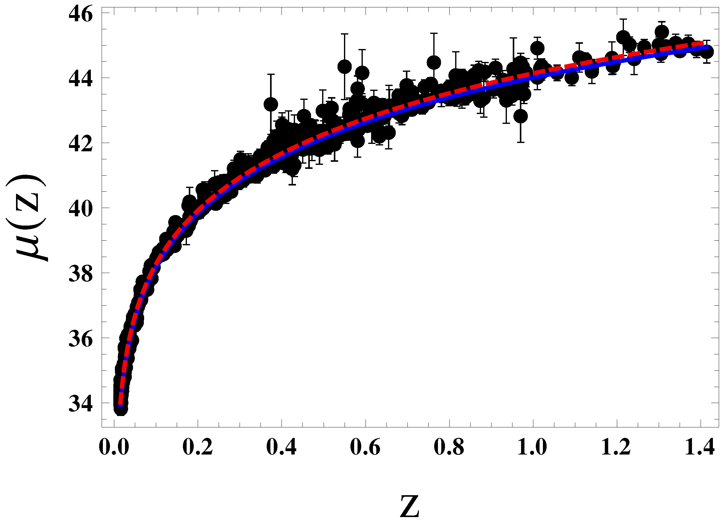
We have shown the evolution of $H(z)$ for the above-mentioned model in Figure 1 by considering the values of the model parameters, as given in Table 1 and compared it with that of the standard $\mathsf{\Lambda }$CDM model. In this figure, we have also plotted the data points for $H(z)$ measurements (within $1\sigma$ error bars) which have been calculated from the latest compilation of 51 data points of $H(z)$ data (for more details, see Ref. [44]). We have observed from Figure 1 that the NGCG model reproduces the observed values of $H(z)$ quite effectively for each data point. Furthermore, in the inset diagram of Figure 1 (left panel), we observed that $\mathsf{\Lambda }$CDM models are negligible around redshift z∼ 0.7. It has also been found that $H_{NGCG}(z)>H_{\mathsf{\Lambda }CDM}(z)$ at low redshifts, while $H_{NGCG}(z)<H_{\mathsf{\Lambda }CDM}(z)$ at relatively high redshifts. These scenarios are in good agreement with a recent work by Mamon and Saha [45], in which they have observed that the relative difference between the models (Lambert W single fluid model &$\mathsf{\Lambda }$CDM model) are negligible around z∼$0.67$. Next, the best fit of distance modulus $\mu (z)$ for the present model (blue line) and the $\mathsf{\Lambda }$CDM model (red line) are plotted in Figure 2. The 580 points of Supernovae Type Ia datasets (black dots) are also plotted in Figure 2 for comparision. From this figure, it has been observed that our model reproduces the observed values of $\mu (z)$ quite effectively.

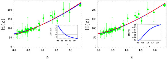
Figure 1. The evolution of the Hubble parameter (blue curve) is shown for the best-fit values of model parameters, as given in Table 1, arising from the joint analysis of $H(z)$ + BAO + CMB + BBN + SNIa (Pantheon) dataset (left panel) and $H(z)$ + BAO + CMB + BBN + SNIa (Union 2.1) dataset (right panel). Here, the red curve represents the corresponding evolution of $H(z)$ in a standard $\mathsf{\Lambda }$CDM model with ${\mathsf{\Omega }}_{cdm0}=0.315$, $H_0=67.4$ km/s/Mpc [40] (left panel) and ${\mathsf{\Omega }}_{cdm0}=0.2675$, $H_0=71.3$ km/s/Mpc [37] (right panel). In this plot, the green dots correspond to the 51 $H(z)$ data points in the redshift range $0.07\le z\le 2.36$, obtained from different surveys and the corresponding $H(z)$ values are given in [44]. In the inset diagram, the corresponding relative difference, $\mathsf{\Delta }H(\%)=100\times (H_{NGCG}(z)-H_{\mathsf{\Lambda }CDM}(z))/H_{\mathsf{\Lambda }CDM}(z)$, is shown for the best-fit model.

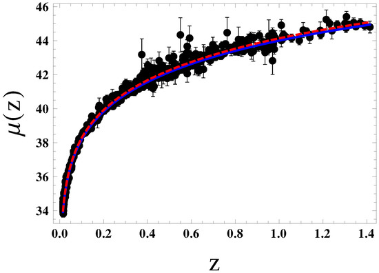
Figure 2. The evolution of $\mu (z)$ is shown for the best-fit values of model parameters, as given in Table 1, arising from the joint analysis of $H(z)$ + BAO + CMB + BBN + SNIa (Union 2.1) dataset (blue curve). The $\mathsf{\Lambda }$CDM model (${\mathsf{\Omega }}_{cdm0}=0.2675$ and $H_0=71.3$ km/s/Mpc [37]) is also shown in the red line for model comparison. Here, $\mu (z)$ represents the distance modulus, which is the difference between the apparent magnitude and the absolute magnitude of the observed supernova, is given by [3] $\mu (z)=25+5{\log }_{10}(d_L/Mpc)$, where $d_L$ is the luminosity distance. In this plot, the black dots correspond to the Error bar plot of 580 points of Union 2.1 compilation Supernovae Type Ia data sets [41].

3. Geometrical Diagnostics

3.1. Statefinder Diagnostics

Since various DE models have been constructed for describing or interpreting the cosmic acceleration, the problem of discriminating between the various DE candidates becomes very important. For this purpose, the authors of [46,47] have introduced a new mathematical diagnostic pair $(r,s)$, known as a statefinder parameter. This diagnostic pair is a “geometrical” in the sense that it depends upon the scale factor directly and hence upon the metric describing space-time. The parameters r and s are defined (in terms of $H(z)$ and its derivatives) as

$$r(z)=\frac{\stackrel{⃛}{a}}{a{H}^3}=1-2(1+z)\frac{H^{\prime }}{H}+\left\{\frac{H^{″}}{H}+{\left(\frac{H^{\prime }}{H}\right)}^2\right\}{(1+z)}^2$$

(12)

$$s(z)=\frac{(r(z)-1)}{3(q(z)-\frac{1}{2})}$$

(13)

It deserves to mention here that different combinations of r and s represent different DE models [46,47]. For example,

• For $\mathsf{\Lambda }$CDM →$(r=1,s=0)$.
• For Quintessence →$(r<1,s>0)$.
• For CG →$(r>1,s<0)$.
• For SCDM →$(r=1,s=1)$.

The evolutionary trajectories in s-r plane of holographic dark energy (HDE) model [19,20,21,22,23,24,25] with future event horizon as IR cut off starts from the point $s=2/3,r=1$ and approaches towards $\mathsf{\Lambda }$CDM fixed point $(s=0, r=1)$ at late time [24]. In the case of a quintessence DE model by taking constant EoS parameter [46,47] and Ricci DE (RDE) model, the curves in s-r plane are vertical [48]. The trajectory in the s-r plane in Chaplygin gas (CG) lie in the regions $s<0,r>1$ [49], while the phantom model with power law potential as well as the quintessence (inverse power-law) models (Q) lie in the regions $s>0,r<1$ [46,47] and approach the $\mathsf{\Lambda }$CDM fixed point in both cases at a late time. The trajectory in s-r plane forms a swirl before reaching the attractor in the coupled quintessence models [50]. Both the Agegraphic DE model [51] and Polytropic gas model [52] show the $\mathsf{\Lambda }$CDM behavior at an early time. The HDE model of DE with the model parameter $c=1$ and the ghost DE model both show the similar behavior in $(s,r)$ plane [53]. This behavior also matches chaplygin gas [26,27], generalized chaplygin gas [30,31,32,54], Yang–Mills [55], new agegraphic [51,56] and HDE [23,24,25] models of DE. In case of the tachyon DE model [57] and HDE model with Granda–Oliveros IR cut-off (new holographic model) [58], the curve of the s-r plane passes through the $\mathsf{\Lambda }$CDM fixed point at the middle of the evolution of the Universe. The trajectories of the s-r plane end at the $\mathsf{\Lambda }$CDM fixed point ($s=0,r=1$) at a late time, starting from matter-dominated (SCDM) $s=1,r=1$ through an arc segment, parabola (downward) in the case of Tsallis holographic dark energy (THDE) model [59,60]. The evolutionary curve of the s-r plane starts and ends at the $\mathsf{\Lambda }$CDM fixed point $(s=0,r=1)$ by making a swirl and shows the Chaplygin gas behaviour in the case of an RHDE model [61]. Recently, one of the authors has investigated the statefinder pair $r(s)$ of SMHDE model, in which it always lies in Chaplygin gas region and approaches the $\mathsf{\Lambda }$CDM fixed point ($r=1,s=0$) in the late time evolution [62]. The evolutionary curve of the s-r plane starts from a cosmological constant and goes around a corner and proceeds towards another endpoint in case of the Tsallis agegraphic dark energy model [63]. In this work, we have also studied the evolution of the $(s,r)$ pair for the NGCG model. However, one can also look into [64,65,66], where the authors have comprehensively discussed about the statefinder pair analysis for various DE models.

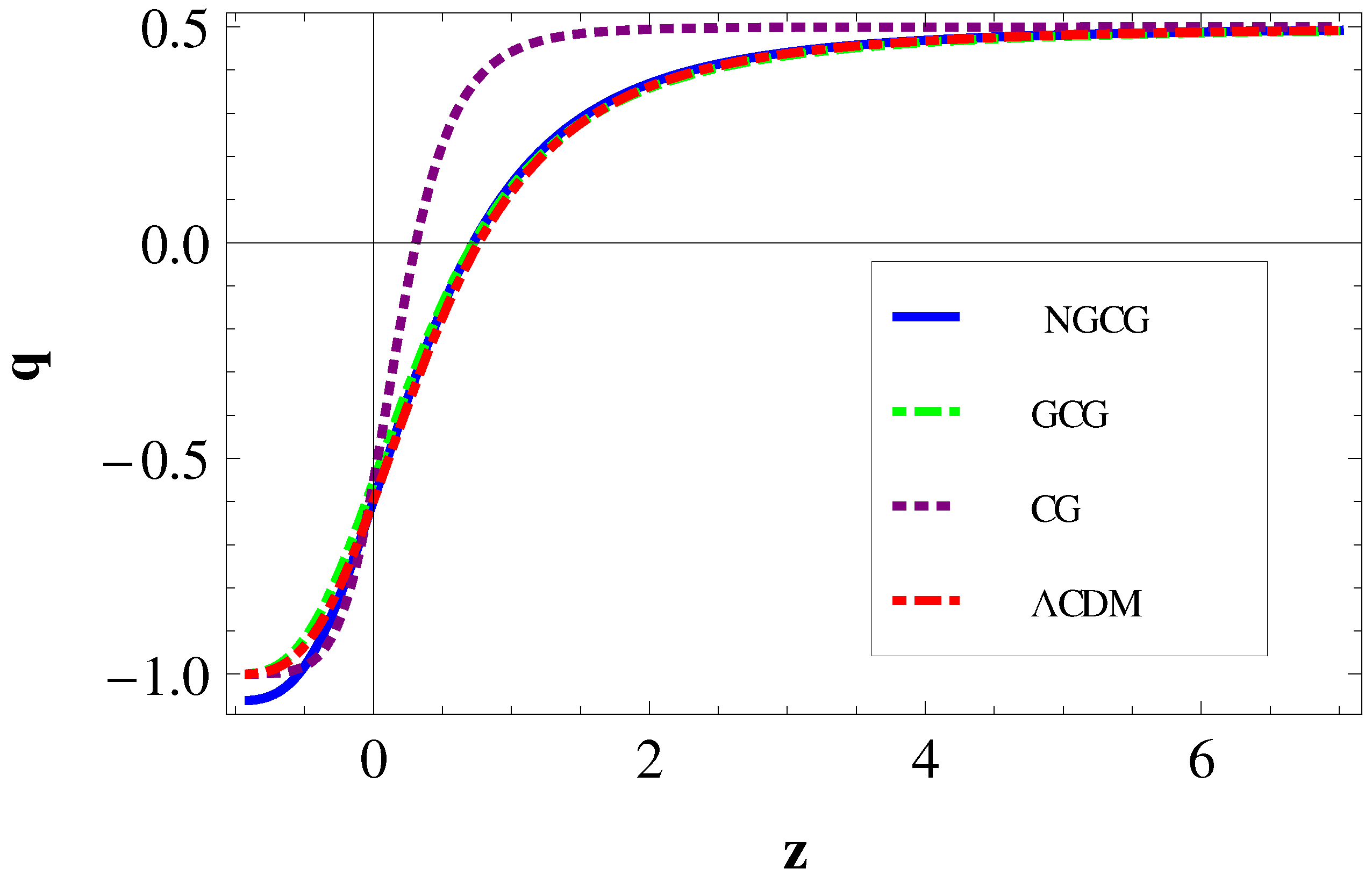
The evolution of the deceleration parameter q against the redshift parameter z, according to the values of the model parameters given in Table 1, is plotted in Figure 3 (blue curve). For comparison, the evolution of q as a function of z for a flat $\mathsf{\Lambda }$CDM, GCG and CG models are also shown. It is observed from Figure 3 that q gives the same prediction of the evolution of the Universe which is undergoing an accelerated expansion phase at the current epoch and experiences a transition from a decelerated expansion phase $(q>0)$ to an accelerated expansion phase $(q<0)$ at the transition redshift $z_t$∼$0.72$ for best-fit values of model parameters. This result is in good agreement with the current cosmological observations ($0.5<z_t<1$) [67,68,69,70,71,72,73].

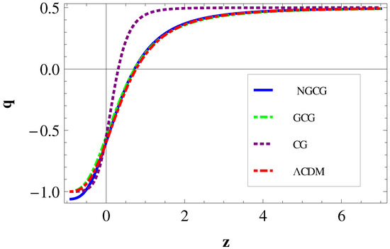
Figure 3. Plot of q as a function of z is shown by considering the values of model parameters, as given in Table 1, arising from the joint analysis of $H(z)$ + BAO + CMB + BBN + SNIa (Pantheon) dataset (blue curve). Here, the red, green, and dotted (purple) curves represent the corresponding evolution of q in a standard $\mathsf{\Lambda }$CDM, GCG, and CG models, respectively.

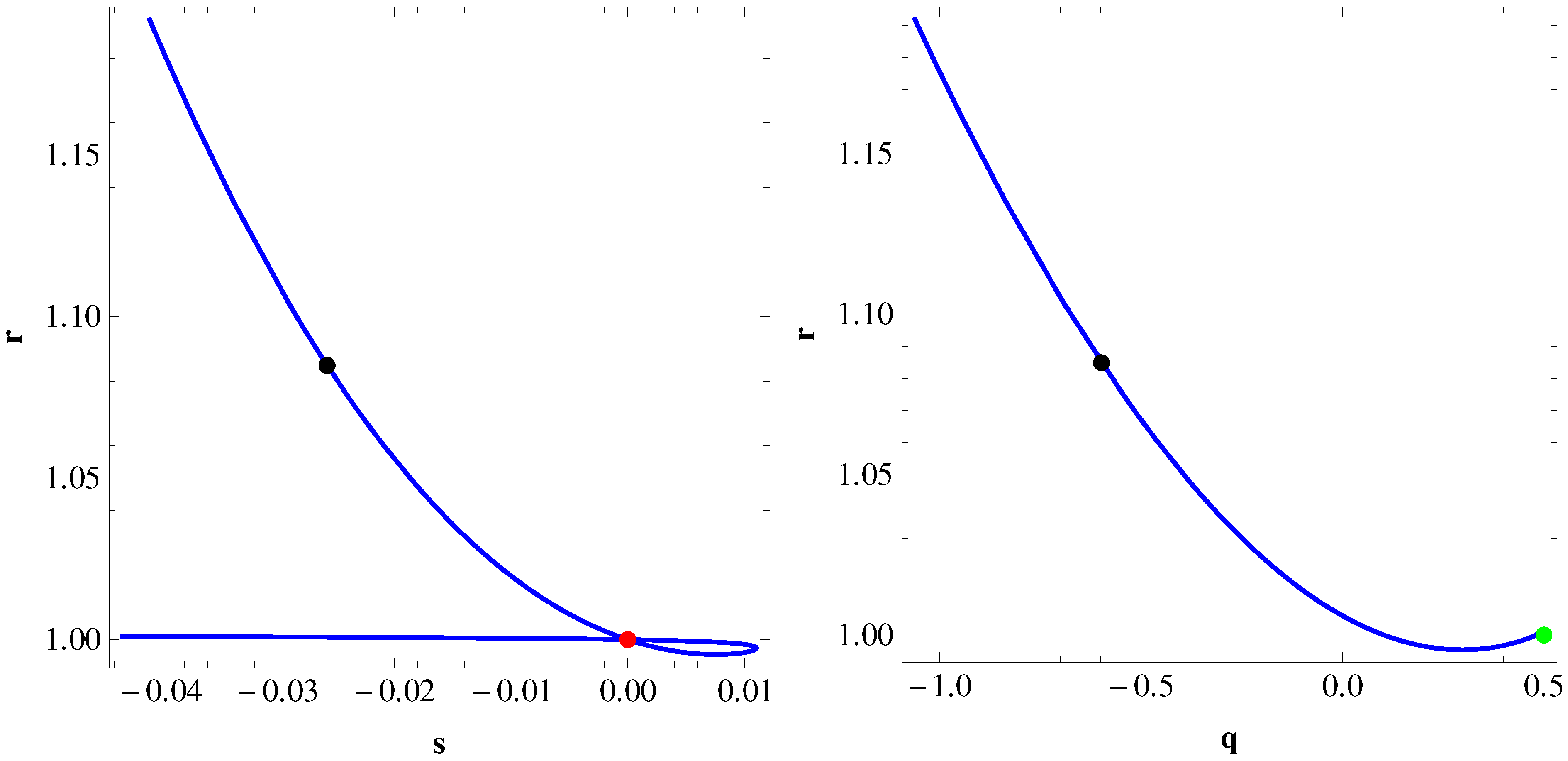
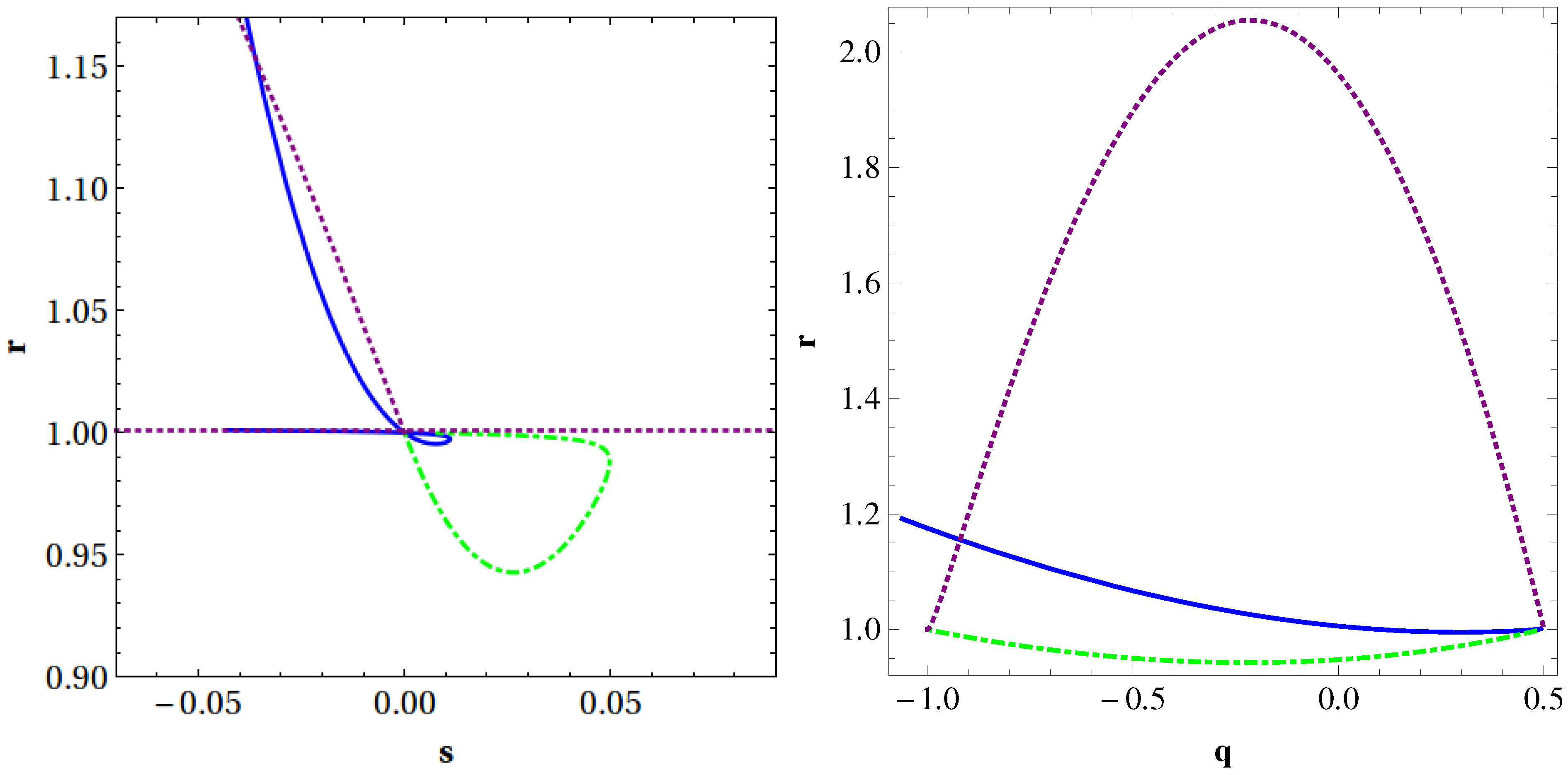
We have reconstructed the evolution of the statefinder pair $(s,r)$ according to the best fitted values of the parameters given in Table 1 for the present model. The plot of statefinder pair $(s,r)$ is shown in the left panel of Figure 4. The evolutionary trajectories of statefinder pair of the NGCG model start its evolution along the line $r=1$ and pass through the $\mathsf{\Lambda }$CDM fixed point ($s=0,r=1$) as time passes. After making a swirl, it lies in the Chaplygin gas region ($s<0,r>1$) in the future for the best-fit values of model parameters, as given in Table 1, arising from the joint analysis of $H(z)$ + BAO + CMB + BBN + SNIa (Pantheon) dataset (blue curve). Hence, Figure 4 shows that the evolutionary trajectories of the statefinder pair of the NGCG model exhibit only the Chaplygin gas behavior and shows different behavior from other DE models. We have also shown the evolutionary trajectories of another statefinder pair $(q,r)$ for the NGCG model in Figure 4 (right panel) for the best-fit values of model parameters, as given in Table 1, arising from the joint analysis of the $H(z)$ + BAO + CMB + BBN + SNIa (Pantheon) dataset. The fixed point ($q=0.5$, $r=1$) corresponds to the SCDM model and the de Sitter expansion is represented by point ($q=-1$, $r=1$) in the q-r plane. The evolutionary curve of the q-r plane of NGCG model starts from the SCDM ( $r=1$, $q=0.5$) in the past and reaches above the de Sitter expansion ($SS$) ($q=-1$, $r=1$) in the future, and it also shows the Chaplygin gas behavior throughout the evaluation. Since q changes its sign from positive to negative, it also reveals the recent phase transition of the Universe. For comparison, the evolutions of $(s,r)$ and $(q,r)$ pair for a NGCG, GCG, and CG models are also shown in Figure 5. Hence, these graphs (Figure 4 and Figure 5) illustrate that, from the statefinder perspective, the NGCG model is different from various other DE models.

Figure 4. The time evolutions of the statefinder pair $(s,r)$ (left panel) and the pair $(q,r)$ (right panel) for this model are shown using the $H(z)$ + BAO + CMB + BBN + SNIa (Pantheon) dataset, as indicated in each panel. The red point $(s=0,r=1)$ in the left panel corresponds to the $\mathsf{\Lambda }$CDM model, while, in the right panel, the green point $(q=0.5,r=1)$ represents the matter dominated Universe (SCDM). In addition, the black dots on the curves show present values $(s_0,r_0)$ (left panel) and $(q_0,r_0)$ (right panel) for the NGCG model.

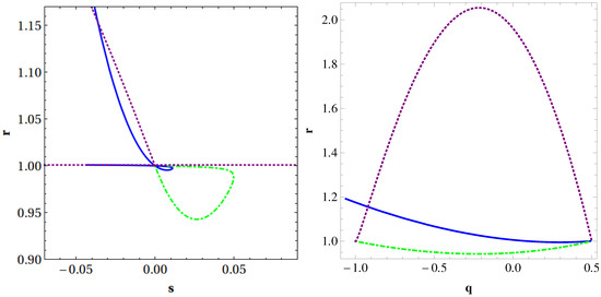
Figure 5. The time evolutions of the statefinder pair $(s,r)$ (left panel) and the pair $(q,r)$ (right panel) for different models are shown using the $H(z)$ + BAO + CMB + BBN + SNIa (Pantheon) dataset. Here, the blue, green, and dotted (purple) curves are for the NGCG, GCG, and CG models, respectively.

3.2. $O_m(z)$ Diagnostics

Another important and useful diagnostic tool constructed from the Hubble parameter is the $O_m$ diagnostic parameter which provides a null test of the standard $\mathsf{\Lambda }$CDM model. Interestingly, constant behavior of $O_m(z)$ with respect to redshift z implies that DE is a cosmological constant (${\omega }_{\mathsf{\Lambda }}=-1$). On the other hand, the positive slope of $O_m(z)$ signifies that DE is phantom (${\omega }_{de}<-1$), whereas the negative slope implies that DE behaves like quintessence (${\omega }_{de}>-1$). Following [74,75], the $O_m(z)$ parameter for a spatially flat Universe is defined as

$$O_m(z)=\frac{{(\frac{H(z)}{H_0})}^2-1}{{(1+z)}^3-1}$$

(14)

Note that it can differentiate a dynamical DE model from the $\mathsf{\Lambda }$CDM model, with and without reference to matter density. For this model, $O_m(z)$ evolves as a function of z as

$$O_m(z)=\frac{(1-{\mathsf{\Omega }}_{r0}-{\mathsf{\Omega }}_{b0}){(1+z)}^3\times {[1-A_s(1-{(1+z)}^{3{\omega }_{de}(1+\alpha )})]}^{\frac{1}{1+\alpha }}+{\mathsf{\Omega }}_{r0}{(1+z)}^4+{\mathsf{\Omega }}_{b0}{(1+z)}^3-1}{{(1+z)}^3-1}$$

(15)

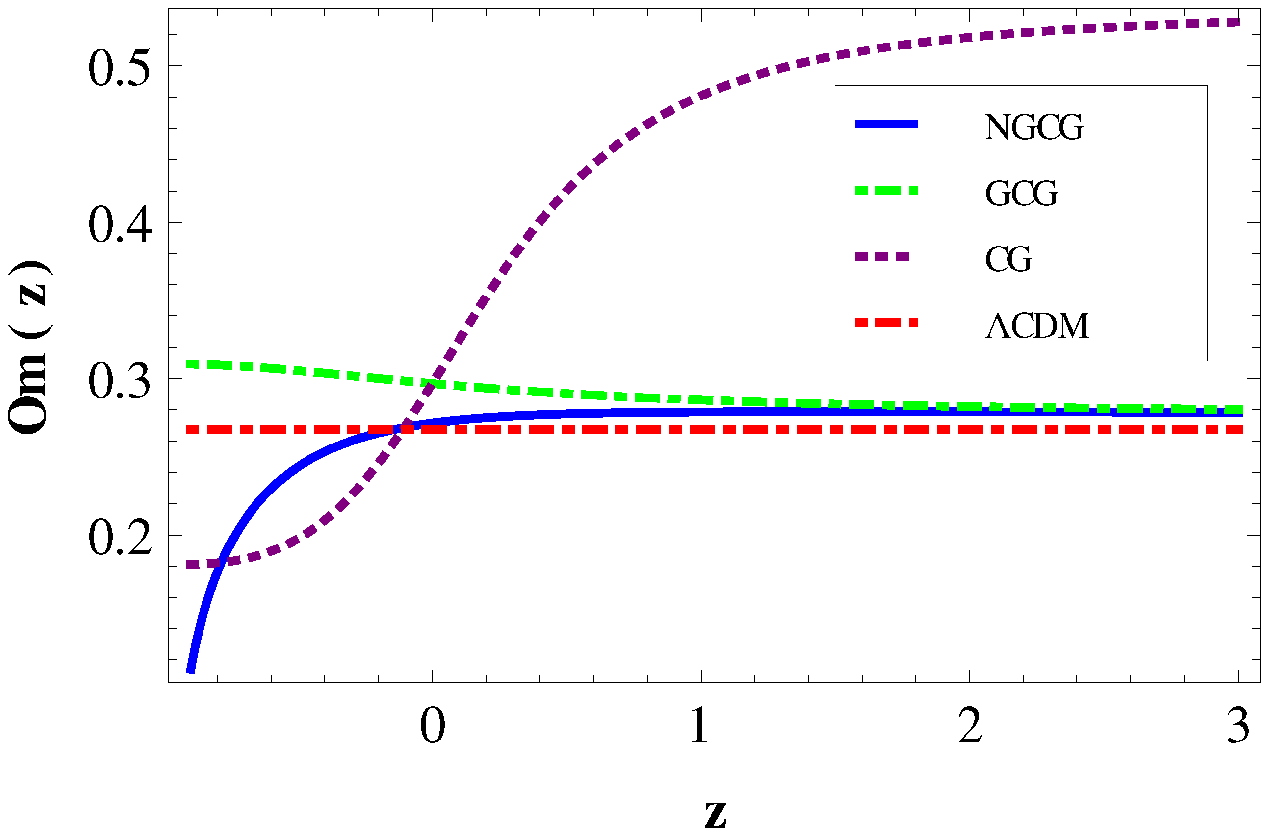
It is evident that, for a spatially flat $\mathsf{\Lambda }$CDM model $O_m(z)={\mathsf{\Omega }}_{m0}$, irrespective of the redshift, which means that, for any two distinct redshifts, say $z_i$ and $z_j$, $O_m(z_i)-O_m(z_j)=0$ is the test for $\mathsf{\Lambda }$CDM. Currently, for any deviation from this condition, a deviation from $\mathsf{\Lambda }$CDM is indicated. The graphical representation of $O_m(z)$ parameter of NGCG model (blue curve) is shown in Figure 6 for the values of model parameters, as given in Table 1, arising from the joint analysis of $H(z)$ + BAO + CMB + BBN + SNIa (Pantheon) dataset. It depicts that the decay of $O_m(z)$ at a lower redshift supports the flourishing DE model.

Figure 6. Evolution of $O_m(z)$ is shown for different models, as indicated in the panel.

4. Conclusions

In the present article, we have examined a new generalized Chaplygin gas (NGCG) model. The main objective of this article is to distinguish the NGCG model from other DE models through the statefinder and $O_m$ diagnostic for the best-fit values of model parameters, as given in Table 1, arising from the joint analysis of $H(z)$ + BAO + CMB + BBN + SNIa (Pantheon) dataset. We can summarize this as:

• We have plotted the deceleration parameter q by getting its numerical solution, which exhibits a transition at $z_t$∼ 0.72, from the early decelerated phase to a late time accelerated phase. This is in good agreement with the current cosmological observations [67,68,69,70,71,72,73].
• The evolutionary curve in the $(s,r)$ plane of NGCG model shows Chaplygin gas behaviour at a late time, while starting its evolution along the line $r=1$ and passes through the $\mathsf{\Lambda }$CDM fixed point ($s=0,r=1$) by making a swirl initially.
• The curve of the q-r plane of the NGCG model shows that it evolves from the matter-dominated Universe i.e., SCDM ( $q=0.5$, $r=1$) initially and approaches above the de Sitter expansion ($SS$) ($q=-1$, $r=1$) at a late time, and it always lies in the Chaplygin gas region throughout the evaluation.
• The evolutionary trajectory of $O_m(z)$ of NGCG model backs the growing DE model.
• Finally, we investigated the evolutions of the Hubble parameter and the distance modulus for the model under consideration and the standard $\mathsf{\Lambda }$CDM model and compare that with the observational datasets (see Figure 1 and Figure 2). For the best-fit case, it has been observed that the relative differences ($\mathsf{\Delta }H$) between the two models (NGCG &$\mathsf{\Lambda }$CDM) are negligible around z∼$0.7$ (see inset diagram of Figure 1 (left panel)). Furthermore, we have found from Figure 2 that the present model reproduces the observed values of the distance modulus quite effectively.

We now conclude that the NGCG model provides some interesting consequences in the cosmological perspective. Furthermore, it would be interesting to investigate the effect on the growth of perturbations for the NGCG model. However, this study lies beyond the scope of the present work and is left for future works.

References

- Riess, A.G.; Filippenko, A.V.; Challis, P.; Clocchiatti, A.; Diercks, A.; Garnavich, P.M.; Gilliland, R.L.; Hogan, C.J.; Jha, S.; Kirshner, R.P.; et al. Observational evidence from supernovae for an accelerating universe and a cosmological constant. Astron. J. 1998, 116, 1009–1038. [Google Scholar] [CrossRef] [Green Version]
- Perlmutter, S.; Aldering, G.; Goldhaber, G.; Knop, R.A.; Nugent, P.; Castro, P.G.; Deustua, S.; Fabbro, S.; Goobar, A.; Groom, D.E.; et al. Measurements of Ω and Λ from 42 high redshift supernovae. Astrophys. J. 1999, 517, 565–586. [Google Scholar] [CrossRef]
- Copeland, E.J.; Sami, M.; Tsujikawa, S. Dynamics of dark energy. Int. J. Mod. Phys. D 2006, 15, 1753–1936. [Google Scholar] [CrossRef] [Green Version]
- Amendola, L.; Tsujikawa, S. Dark Energy: Theory and Observations; Cambridge University Press: Cambridge, UK, 2010. [Google Scholar]
- Bamba, K.; Capozziello, S.; Nojiri, S.; Odintsov, S.D. Dark energy cosmology: The equivalent description via different theoretical models and cosmography tests. Astrophys. Space Sci. 2012, 342, 155–228. [Google Scholar] [CrossRef] [Green Version]
- Weinberg, S. The cosmological constant problem. Rev. Mod. Phys. 1989, 61, 1–23. [Google Scholar] [CrossRef]
- Steinhardt, P.J.; Wang, L.; Zlatev, I. Cosmological tracking solutions. Phys. Rev. D 1999, 59, 123504. [Google Scholar] [CrossRef] [Green Version]
- Riess, A.G.; Macri, L.M.; Hoffmann, S.L.; Scolnic, D.; Casertano, S.; Filippenko, A.V.; Tucker, B.E.; Reid, M.J.; Jones, D.O.; Silverman, J.M.; et al. A 2.4% determination of the local value of the Hubble constant. Astrophys. J. 2016, 826, 56. [Google Scholar] [CrossRef]
- Riess, A.G.; Casertano, S.; Yuan, W.; Macri, L.M.; Scolnic, D. Large Magellanic Cloud Cepheid Standards Provide a 1% Foundation for the Determination of the Hubble Constant and Stronger Evidence for Physics beyond ΛCDM. Astrophys. J. 2019, 876, 85. [Google Scholar] [CrossRef]
- Font-Ribera, A.; Kirkby, D.; Busca, N.; Miralda-Escudé, J.; Ross, N.P.; Slosar, A.; Rich, J.; Aubourg, É.; Bailey, S.; Bhardwaj, V.; et al. Quasar-Lyman α Forest Cross-Correlation from BOSS DR11: Baryon Acoustic Oscillations. JCAP 2014, 05, 027. [Google Scholar] [CrossRef]
- Perivolaropoulos, L.; Skara, F. Challenges for ΛCDM: An update. arXiv 2021, arXiv:2105.05208. [Google Scholar]
- Di Valentino, E.; Mena, O.; Pan, S.; Mena, L.; Yang, W.; Melchiorri, A.; Mota, D.F.; Riess, A.G.; Silk, J. In the Realm of the Hubble tension- a Review of Solutions. arXiv 2021, arXiv:2103.01183. [Google Scholar]
- Sahni, V.; Starobinsky, A. The Case for a positive cosmological Lambda term. Int. J. Mod. Phys. D 2000, 9, 373–444. [Google Scholar] [CrossRef]
- Caldwell, R.R.; Kamionkowski, M.; Weinberg, N.N. Phantom Energy: Dark Energy with w < −1 Causes a Cosmic Doomsday. Phys. Rev. Lett. 2003, 91, 071301. [Google Scholar]
- Armendariz-Picon, C.; Mukhanov, V.; Steinhardt, P.J. A dynamical solution to the problem of a small cosmological constant and late time cosmic acceleration. Phys. Rev. Lett. 2000, 85, 4438–4441. [Google Scholar] [CrossRef] [Green Version]
- Chiba, T.; Okabe, T.; Yamaguchi, M. Kinetically driven quintessence. Phys. Rev. D 2000, 62, 023511. [Google Scholar] [CrossRef] [Green Version]
- Sami, M.; Chingangbam, P.; Qureshi, T. Aspects of tachyonic inflation with an exponential potential. Phys. Rev. D 2002, 66, 043530. [Google Scholar] [CrossRef] [Green Version]
- Padmanabhan, T.; Choudhury, T.R. Can the clustered dark matter and the smooth dark energy arise from the same scalar field? Phys. Rev. D 2002, 66, 081301. [Google Scholar] [CrossRef] [Green Version]
- Hooft, G.T. Dimensional reduction in quantum gravity. Conf. Proc. C 1993, 930308, 284–296. [Google Scholar]
- Susskind, L. The World as a hologram. J. Math. Phys. 1995, 36, 6377–6396. [Google Scholar] [CrossRef] [Green Version]
- Cohen, A.G.; Kaplan, D.B.; Nelson, A.E. Effective field theory, black holes, and the cosmological constant. Phys. Rev. Lett. 1999, 82, 4971–4974. [Google Scholar] [CrossRef] [Green Version]
- Li, M. A Model of holographic dark energy. Phys. Lett. B 2004, 603, 1–5. [Google Scholar] [CrossRef]
- Setare, M.R.; Zhang, J.; Zhang, X. Statefinder diagnosis in a non-flat universe and the holographic model of dark energy. JCAP 2007, 0703, 007. [Google Scholar] [CrossRef] [Green Version]
- Zhang, X. Statefinder diagnostic for holographic dark energy model. Int. J. Mod. Phys. D 2005, 14, 1597–1606. [Google Scholar] [CrossRef]
- Zhang, J.; Zhang, X.; Liu, H. Statefinder diagnosis for the interacting model of holographic dark energy. Phys. Lett. B 2008, 659, 26–33. [Google Scholar] [CrossRef] [Green Version]
- Kamenshchik, A.; Moschella, U.; Pasquier, V. An alternative to quintessence. Phys. Lett. B 2001, 511, 265. [Google Scholar] [CrossRef] [Green Version]
- Gorini, V.; Kamenshchik, A.; Moschella, U. Can the Chaplygin gas be a plausible model for dark energy? Phys. Rev. D 2003, 67, 063509. [Google Scholar] [CrossRef] [Green Version]
- Bean, R.; Dore, O. Are Chaplygin gases serious contenders for the dark energy? Phys. Rev. D 2003, 68, 023515. [Google Scholar] [CrossRef] [Green Version]
- Sandvik, H.B.; Tegmark, M.; Zaldarriaga, M.; Waga, I. The end of unified dark matter? Phys. Rev. D 2004, 69, 123524. [Google Scholar] [CrossRef]
- Bento, M.C.; Bertolami, O.; Sen, A.A. Generalized Chaplygin gas, accelerated expansion and dark energy matter unification. Phys. Rev. D 2002, 66, 043507. [Google Scholar] [CrossRef] [Green Version]
- Bento, M.C.; Bertolami, O.; Sen, A.A. Revival of the unified dark energy-dark matter model? Phys. Rev. D. 2004, 70, 083519. [Google Scholar] [CrossRef] [Green Version]
- Fabris, J.C.; Goncalves SV, B.; de Sá Ribeiro, R. Generalized Chaplygin gas with alpha = 0 and the lambda-CDM cosmological model. Gen. Rel. Grav. 2004, 36, 211–216. [Google Scholar] [CrossRef] [Green Version]
- Barreiro, T.; Bertolami, O.; Torres, P. WMAP five-year data constraints on the unified model of dark energy and dark matter. Phys. Rev. D 2008, 78, 043530. [Google Scholar] [CrossRef] [Green Version]
- Zhang, X.; Wu, F.Q.; Zhang, J. New generalized Chaplygin gas as a scheme for unification of dark energy and dark matter. JCAP 2006, 0601, 003. [Google Scholar] [CrossRef]
- Liao, K.; Pan, Y.; Zhu, Z.H. Observational constraints on new generalized Chaplygin gas model. Res. Astron. Astrophys. 2013, 13, 159–169. [Google Scholar] [CrossRef] [Green Version]
- Wang, J.; Wu, Y.B.; Wang, D.; Yang, W.Q. The Extended Analysis on New Generalized Chaplygin Gas. Chin. Phys. Lett. 2009, 26, 089801. [Google Scholar]
- Salahedin, F.; Pazhouhesh, R.; Malekjani, M. Cosmological constrains on new generalized Chaplygin gas model. Eur. Phys. J. Plus 2020, 135, 429. [Google Scholar] [CrossRef]
- Yang, W.; Pan, S.; Paliathanasis, A.; Ghosh, S.; Wu, Y. Observational constraints of a new unified dark fluid and the H0 tension. arXiv 2019, arXiv:1904.10436. [Google Scholar] [CrossRef]
- Yang, W.; Pan, S.; Vagnozzi, S.; Di Valentino, E.; Mota, D.F.; Capozziello, S. Dawn of the dark: Unified dark sectors and the EDGES Cosmic Dawn 21-cm signal. arXiv 2019, arXiv:1907.05344. [Google Scholar] [CrossRef] [Green Version]
- Aghanim, N.; Akrami, Y.; Ashdown, M.; Aumont, J.; Baccigalupi, C.; Ballardini, M.; Banday, A.J.; Barreiro, R.B.; Bartolo, N.; Basak, S.; et al. Planck 2018 results. VI. Cosmological parameters. Astron. Astrophys. 2020, 641, A6. [Google Scholar]
- Suzuki, N.; Rubin, D.; Lidman, C.; Aldering, G.; Amanullah, R.; Barbary, K.; Barrientos, L.F.; Botyanszki, J.; Brodwin, M.; Connolly, N.; et al. The Hubble Space Telescope Cluster Supernova Survey: V. Improving the Dark Energy Constraints Above z > 1 and Building an Early-Type-Hosted Supernova Sample. Astrophys. J. 2012, 746, 85. [Google Scholar] [CrossRef] [Green Version]
- Scolnic, D.M.; Jones, D.O.; Rest, A.; Pan, Y.C.; Chornock, R.; Foley, R.J.; Huber, M.E.; Kessler, R.; Narayan, G.; Riess, A.G.; et al. The Complete Light-curve Sample of Spectroscopically Confirmed SNe Ia from Pan-STARRS1 and Cosmological Constraints from the Combined Pantheon Sample. Astrophys. J. 2018, 859, 101. [Google Scholar] [CrossRef]
- Cooke, R.J.; Pettini, M.; Steidel, C.C. One Percent Determination of the Primordial Deuterium Abundance. Astrophys. J. 2018, 855, 102. [Google Scholar] [CrossRef] [Green Version]
- Magana, J.; Amante, M.H.; Garcia-Aspeitia, M.A.; Motta, V. The Cardassian expansion revisited: Constraints from updated Hubble parameter measurements and type Ia supernova data. Mon. Not. R. Astron. Soc. 2018, 476, 1036–1049. [Google Scholar] [CrossRef]
- Al Mamon, A.; Saha, S. Testing lambert W equation of state with observational hubble parameter data. New Astron. 2021, 86, 101567. [Google Scholar] [CrossRef]
- Sahni, V.; Saini, T.D.; Starobinsky, A.A.; Alam, U. Statefinder—A new geometrical diagnostic of dark energy. J. Exp. Theor. Phys. Lett. 2003, 77, 201–206. [Google Scholar] [CrossRef]
- Alam, U.; Sahni, V.; Saini, T.D.; Starobinsky, A.A. Exploring the Expanding Universe and Dark Energy using the Statefinder Diagnostic. Mon. Not. R. Astron. Soc. 2003, 344, 1057. [Google Scholar] [CrossRef]
- Feng, C.J. Statefinder Diagnosis for Ricci Dark Energy. Phys. Lett. B 2008, 670, 231–234. [Google Scholar] [CrossRef] [Green Version]
- Wu, Y.B.; Li, S.; Fu, M.H.; He, J. A modified Chaplygin gas model with interaction. Gen. Rel. Grav. 2007, 39, 653–662. [Google Scholar] [CrossRef]
- Zhang, X. Statefinder diagnostic for coupled quintessence. Phys. Lett. B 2005, 611, 1–7. [Google Scholar] [CrossRef] [Green Version]
- Zhang, L.; Cui, J.; Zhang, J.; Zhang, X. Interacting model of new agegraphic dark energy: Cosmological evolution and statefinder diagnostic. Int. J. Mod. Phys. D 2010, 19, 21–35. [Google Scholar] [CrossRef] [Green Version]
- Malekjani, M.; Mohammadi, A.K. Statefinder diagnostic and w − w′ analysis for interacting polytropic gas dark energy model. Int. J. Theor. Phys. 2012, 51, 3141–3151. [Google Scholar] [CrossRef]
- Malekjani, M.; Mohammadi, A.K. Statefinder diagnosis and the interacting ghost model of dark energy. Astrophys. Space Sci. 2013, 343, 451–461. [Google Scholar] [CrossRef] [Green Version]
- Malekjani, M.; Zarei, R.; Jafarpour, M.H. Holographic dark energy with time varying model parameter c2(z). Astrophys. Space Sci. 2013, 343, 799–806. [Google Scholar] [CrossRef] [Green Version]
- Zhao, W. Statefinder diagnostic for Yang-Mills dark energy model. Int. J. Mod. Phys. D 2008, 17, 1245–1254. [Google Scholar] [CrossRef] [Green Version]
- Mohammadi, A.K.; Malekjani, M. Cosmic Behavior, Statefinder Diagnostic and w − w′ Analysis for Interacting NADE model in Non-flat Universe. Astrophys. Space Sci. 2011, 331, 265–273. [Google Scholar] [CrossRef] [Green Version]
- Shao, Y.; Gui, Y. Statefinder parameters for tachyon dark energy model. Mod. Phys. Lett. A 2008, 23, 65–71. [Google Scholar] [CrossRef] [Green Version]
- Malekjani, M.; Mohammadi, A.K.; Nazari-pooya, N. Cosmological evolution and statefinder diagnostic for new holographic dark energy model in non flat universe. Astrophys. Space Sci. 2011, 332, 515–524. [Google Scholar] [CrossRef] [Green Version]
- Tavayef, M.; Sheykhi, A.; Bamba, K.; Moradpour, H. Tsallis Holographic Dark Energy. Phys. Lett. B 2018, 781, 195–200. [Google Scholar] [CrossRef]
- Sharma, U.K.; Pradhan, A. Diagnosing Tsallis holographic dark energy models with statefinder and ω − ω′. pair. Mod. Phys. Lett. A 2019, 34, 1950101. [Google Scholar] [CrossRef]
- Sharma, U.K.; Dubey, V.C. Statefinder diagnostic for the Renyi holographic dark energy. New Astron. 2020, 80, 101419. [Google Scholar] [CrossRef]
- Upadhyay, S.; Dubey, V.C. Diagnosing the Sharma-Mittal Holographic Dark Energy Model through the Statefinder. Gravit. Cosmol. 2021, 27, 281–291. [Google Scholar] [CrossRef]
- Srivastava, S.; Dubey, V.C.; Sharma, U.K. Statefinder diagnosis for Tsallis agegraphic dark energy model with ωD − ωD′ pair. Int. J. Mod. Phys. A 2020, 35, 2050027. [Google Scholar] [CrossRef]
- Sami, M.; Shahalam, M.; Skugoreva, M.; Toporensky, A. Cosmological dynamics of a nonminimally coupled scalar field system and its late time cosmic relevance. Phys. Rev. D 2012, 86, 103532. [Google Scholar] [CrossRef] [Green Version]
- Myrzakulov, R.; Shahalam, M. Statefinder hierarchy of bimetric and galileon models for concordance cosmology. JCAP 2013, 10, 047. [Google Scholar] [CrossRef] [Green Version]
- Rani, S.; Altaibayeva, A.; Shahalam, M.; Singh, J.K.; Myrzakulov, R. Constraints on cosmological parameters in power-law cosmology. JCAP 2015, 03, 031. [Google Scholar] [CrossRef] [Green Version]
- Farooq, O.; Ratra, B. Hubble parameter measurement constraints on the cosmological deceleration-acceleration transition redshift. Astrophys. J. 2013, 766, L7. [Google Scholar] [CrossRef]
- Ishida, E.E.; Reis, R.R.; Toribio, A.V.; Waga, I. When did cosmic acceleration start? How fast was the transition? Astropart. Phys. 2008, 28, 547–552. [Google Scholar] [CrossRef] [Green Version]
- Magaña, J.; Cárdenas, V.H.; Motta, V. Cosmic slowing down of acceleration for several dark energy parametrizations. J. Cosmol. Astropart. Phys. 2014, 10, 017. [Google Scholar] [CrossRef] [Green Version]
- Al Mamon, A.; Bamba, K.; Das, S. Constraints on reconstructed dark energy model from SN Ia and BAO/CMB observations. Eur. Phys. J. C 2017, 77, 29. [Google Scholar] [CrossRef] [Green Version]
- Al Mamon, A. Constraints on a generalized deceleration parameter from cosmic chronometers. Mod. Phys. Lett. A 2018, 33, 1850056. [Google Scholar] [CrossRef] [Green Version]
- Al Mamon, A.; Das, S. A parametric reconstruction of the deceleration parameter. Eur. Phys. J. C 2017, 77, 495. [Google Scholar] [CrossRef]
- Al Mamon, A. Constraints on kinematic model from Pantheon SNIa, OHD and CMB shift parameter measurements. Mod. Phys. Lett. A 2021, 36, 2150049. [Google Scholar] [CrossRef]
- Sahni, V.; Shafieloo, A.; Starobinsky, A.A. Two new diagnostics of dark energy. Phys. Rev. D 2008, 78, 103502. [Google Scholar] [CrossRef] [Green Version]
- Zunckel, C.; Clarkson, C. Consistency Tests for the Cosmological Constant. Phys. Rev. Lett. 2008, 101, 181301. [Google Scholar] [CrossRef] [PubMed] [Green Version]
Publisher’s Note: MDPI stays neutral with regard to jurisdictional claims in published maps and institutional affiliations. |
© 2021 by the authors. Licensee MDPI, Basel, Switzerland. This article is an open access article distributed under the terms and conditions of the Creative Commons Attribution (CC BY) license (https://creativecommons.org/licenses/by/4.0/).