Abstract
In this paper, we investigate the stability and feasibility of an anisotropic stellar model under gravity that embraces the Karmarkar condition. In order to develop the gravity model, the functional form of is taken into consideration as the linear function of the trace of the energy-momentum tensor T and the Ricci scalar R, respectively. This study proposes a well-known form of the radial metric function and finds another metric function by employing the Karmakar condition, which provides the exact solution to the field equation. The expression of the model parameters is derived by matching the obtained interior solutions with the Schwarzschild exterior metric over the bounding surface of a celestial object, along with the requirement that the radial pressure vanish at the boundary. The current estimated data of the star, pulsar 4U1608-52, is used to graphically explore the model. The physical attributes of the celestial object are thoroughly examined within the framework of the present model. Adjusting the model parameter, a detailed analysis of the stability criterion is presented that involves the adiabatic index, the Herrera cracking technique, and the causality condition. Furthermore, the Tolman–Oppenheimer–Volkhoff equation is used to analyze the stellar model’s equilibrium state. In order to maintain the stability condition of the anisotropic stellar structure, a suitable range for the model parameter is determined by the graphical analysis of the present model in this study. In addition, the numerical values of the physical parameters related to the compact stars Her X-1, LMC X-4, Cen X-3 and KS1731-207 are used to examine the model solution within the desired range of the model parameter.
1. Introduction
In order to clarify the spacetime curvature caused by matter and energy and to reveal the connection between the matter distribution and the gravitational force brought on by this curvature, Albert Einstein established the novel theoretical concept known as the General Theory of Relativity. These scenarios are designed by a set of dynamical equations called the Einstein field equation. To study the physical features as well as to examine the stability of stellar objects, the solution of the field equation is necessary to obtain. In 1916, Schwarzschild [1] derived the exact solution of Einstein’s field equation in vacuum space, which describes the space-time geometry in the exterior region of a spherically symmetric matter distribution. According to certain empirical studies, most of the invisible matter of the universe can be recognized by its gravitational influence even though it is neither luminous nor radiation. Such a mass is referred to as dark matter. Additionally, the study indicates that just one-third of the mass of the universe is included in visible matter and detectable radiation. The remaining two-thirds of the matter density of the universe is known as dark energy, and it exists in some unclustered form.
The wide-ranging presence of dark matter and dark energy throughout the universe creates significant theoretical obstacles to Einstein’s gravity model. In recent years, several researchers have developed the concept of modified theories of gravity to overcome these limitations of Einstein’s theory of general relativity. One of the well-known modified theories is the theory of gravity [2,3], in which the Hilbert action is taken as a nonlinear analytic function of the Ricci scalar R. Another significant modified theory is teleparallel gravity, which creates a null-curvature with a non-vanishing torsion by adopting the Weitzenbock connection [3,4,5]. The field equations of teleparallel gravity are developed using the tetrad field, which acts as the dynamical variables of the theory, and the torsion scalars, which describe the effect of gravity [6,7]. Modifying the action of teleparallel gravity, the gravity model is designed using an extensible torsion scalar function [8,9]. Unlike the metric used in general relativity, the main fields in this gravitational theory are tetrads. In addition, numerous researchers have created a number of expanded variants of the modified theories of gravity mentioned above. For example, etc. [10,11,12,13,14,15,16,17,18,19,20,21,22]. Nevertheless, by generalizing theory, Harko et al. [10] considered an arbitrary coupling between matter and spacetime geometry in the form , where T is the trace of the energy-momentum tensor and R is the Ricci scalar.
Earlier, it was believed that a spherically symmetric object has a nature similar to that of a perfect fluid, in which the radial and tangential pressure coincide. Surprisingly, this idea was altered by Jean’s revolutionary work [23], which proposed that anisotropic pressure should be taken into account because of the intense and unfamiliar conditions existing inside the compact structure. Later many researchers agreed with the fact that there are a variety of phenomena that occur in spherically symmetric objects, which may result in different pressure along the radial direction ( and in orthogonal direction (). For instance, Weber [24] claims that changes in the magnetic field’s strength during neutron star evolution result in pressure anisotropy. Sawyer [25] and Sokolov [26] found that pion condensation and phase transition can also result in anisotropic pressure. Likewise, anisotropy is crucial for examining the physical characteristics of celestial objects. To investigate the anisotropic strange star, the researchers used the embedding approach in the work [27] under the most simple linear function of the matter-geometric coupling. By applying the Tolman–Kuchowicz metric potential, an analysis of an anisotropic spherically symmetric strange star was conducted by the researchers in [28]. In the condition of pressure anisotropy, Paul and Deb [29] analyzed the feasible features of the stellar object. Anisotropy’s effects on relativistic objects and the acceptability of the anisotropic model were investigated by Bowers and Liang [30].
Multiple strategies have been used to obtain the solution of anisotropic stellar models, such as assuming the expression for anisotropy, considering constraints on fluid parameters, and a specific form of equation of state parameters. Unlike the above approaches, another well-known technique, the Karmarkar condition [31], is incorporated to solve the model constraint in this present work. The Karmarkar condition furnishes a simple integral relation between the metric functions and their derivatives. Consequently, one can assume one of the metric functions to determine another one by applying this condition. The Karmarkar condition offers a geometrical way to use equations of state that link the tangential and radial pressures. Sharif and Gul [32] examine the physical characteristics of self-gravitating objects in the presence of anisotropic matter distribution, adopting the Karmarkar condition in energy-momentum squared gravity. Nazeer and Feroze [33] used Karmarkar–Bardeen to find an innovative class-I solution of the field equation in gravity for the charged anisotropic spherically symmetric matter distribution. Being motivated by all of the previous research works [31,32,33,34,35,36], the current paper aims to study compact stellar objects in gravity using the Karmarkar condition.
In the paper [37], E. Battista et. al. developed a unique class of static and spherically symmetric Casimir WHs incorporating GUP modifications within the context of RR gravity. Specifically, the Herrera cracking technique, which is used to assess WH stability, has the potential to generate significant insights in the subject of wormhole geometries. T. Naseer and colleagues examined traversable WH geometries in the framework of theory in the article [38]. They used the Karmarkar condition to determine a WH form function and assess its viability. The study [39] analyzed the viable traversable wormhole solutions through Karmarkar condition in the setting of theory. In the paper [39], the authors employed Karmarkar condition to design a valid shape function for a static wormhole structure. Driven by these previous works, in this study we examine an uncharged superdense compact stellar object under gravity employing the Karmarkar condition coupled with Vaidya–Tikekar approach. This idea offers novel insights concerning its recent work. The impact of the VT metric’s spheroidal parameter K on the physical characteristics of different compact objects is also reflected in this study. The dependence of the model parameter on key physical quantities such as density and pressure is explicitly demonstrated in our model. Furthermore, the parameter can be fine-tuned to match recent observational data from various pulsar sources. These are the distinctive attributes of this research.
The structure of this present work is thus as follows: The modified field equations for the anisotropic uncharged stellar model are declared in Section 2. The Karmarkar condition is employed in solving the modified field equations of the present anisotropic model in Section 3. Section 4 provides the expressions for model constants by matching the interior solution of the model with the Schwarzschild’s exterior vacuum solution at the boundary. The different subsections of Section 5 present a graphical analysis of the metric functions’ nature, the state parameters’ different aspects, and the energy conditions. A brief discussion on stability analysis for the model has been made via adiabatic index, causality requirement, and Herrera cracking method in Section 6. Section 7 explained the equilibrium state of the present stellar model through the TOV equation. The work is concluded with some remarkable observations on model parameter in Section 8.
2. Modified Field Equation in Gravity
The theory of gravity is a modification of the Einstein–Hilbert action, which has the following form:
where is an arbitrary function of the Ricci curvature R and the trace of the energy-momentum tensor T, and represents the trace of the energy-momentum tensor and the Lagrangian associated with the distribution of matter, respectively. Here, also, g stands for the determinant of the metric tensor .
The energy-momentum tensor is defined as
and is known as the trace of , where is the usual gravitational metric.
As stated in [10], the Lagrangian for the matter distribution depends only on and not on its derivatives; this shows that
Using the variational principle, the field equation is obtained from the action (1) as
where and represent the derivative of with respect to R and T, respectively. In this case, and □ represent the covariant derivative with respect to the metric tensor and the D’Alembertian operator, respectively. Here, □ and are expressed as follows:
Using Equation (3), the tensor can be expressed as
Moreover, the anisotropic matter distribution is defined as follows:
where , and represent the energy density, the radial pressure, and the transverse pressure, respectively.
denotes the four-vector in the radial direction with and refers to the four-velocity with and .
The relation between Lagrangian matter and isotropic pressure can be considered as
According to [10], using the relation (8) in Equation (6) implies that
In addition to the effective energy-momentum tensor , the aforementioned field Equation (4) can also be defined in gravity in the form of the Einstein tensor as
where and can be expressed as
and
where represents the usual matter energy-momentum tensor and denotes the corrections appeared due to modification of gravity theory and also further expressed as
The internal spacetime of a stellar object is assumed to be well represented by the following metric, which is provided by
By using a specific model in the context of modified theory, scientists are able to get over GR’s limitations in explaining a variety of cosmic occurrences. In order to study a stellar model in the modified theory of gravity, the function is considered as follows:
Combining the metric (12) with Equations (7), (10) and (13) the basic field equations are obtained as follows (taking ):
Numerous researchers have previously employed a variety of approaches to find solutions to field equations in different theories of gravity. Accurately solving those equations in the theory of gravity may be difficult. With a similar type of initial assumption, several authors have discovered solutions applying the Karmakar condition [40]. By incorporating the Vaidya–Tikekar ansatz [41], the present work generates a logically valid solution.
By solving the field Equations (14)–(16) simultaneously, the fluid density , the fluid radial pressure , and the fluid transversal pressure are explicitly obtained as
where ,
and
Fluctuation of the pressure in various directions within a fluid distribution is referred to as anisotropic pressure. In this study, the expression of anisotropy is given by
3. Solutions of Stellar Model in Theory Using Karmarkar Condition
The goal of this study is to develop a new anisotropic model for stellar objects for the theory of gravity. There are three equations and five unknowns, namely , and in the system of field Equations (17)–(19). For the sake of consistency, two additional relations must be taken into account in order to match the number of equations with the number of unknowns of the aforementioned system of equations.
The Karmarkar condition [31] is used to solve the field equations. According to the general theory of relativity, ‘p’ is said to be the embedding class whenever an n-dimensional spacetime is embedded in a pseudo-Euclidean spacetime of spacetime [42]. It is widely acknowledged that if a symmetric tensor of a four-dimensional Riemannian space meets the Gauss [43] and Codazzi [44] constraints:
then it can be embedded in a five-dimensional pseudo-Euclidean space, where takes the value or depending on whether the normal to the manifold is space-like or time-like, and the symbol ‘;’ stands for covariant derivatives.
The components of the Riemann curvature tensor in regard to the line element in (12) can be expressed as
It is manifested that the non-zero components of the tensor are and also due to its symmetric nature and . Using the aforementioned components the necessary Karmarkar condition can be expressed as:
According to Sharma and Pandey [45], the Karmarkar requirement (21) and are sufficient conditions for a spacetime to be a class one spacetime. When the nonzero components of the Riemann curvature tensor are substituted in Equation (21), the following differential equation can be obtained as:
By solving the above differential equation, the relationship between the metric components can be found as
where C and D are integrating constants that will be obtained by the boundary conditions.
In order to explain the superdense and realistic stellar interior, such as neutron stars, Vaidya and Tikekar’s approach [41] can be taken into account. In this study, the static spherically symmetric space-time is analyzed using the VT metric function as follows:
where K is a dimensionless parameter that quantifies the degree of ellipticity of the star and L is a curvature parameter with a dimension of length.
4. Matching Conditions at the Stellar Boundary
The interior geometry and exterior geometry of a star must be smoothly linked for a stellar structure to exist physically. Any stable, spherically symmetric celestial object must have a smooth, continuous stellar distribution at its surface between the interior and the outer solutions . According to the Jebsen–Birkhoff theorem [46], the Schwarzschild solution is the only spherically symmetric solution to the vacuum Einstein field equations in general relativity. In that scenario, a spherically symmetric gravitational field outside a spherical stellar object in empty space must be asymptotically flat and static. According to the continuity of the first fundamental form, the interior solution and the vacuum exterior Schwarzschild solution at the boundary must match smoothly.
The Schwarzschild metric can be used to characterize the external spacetime of a non-radiating star and is provided as
where , M being the mass of the star. At the boundary, the continuations of the first and second fundamental forms yield the following relations:
Taking into account the space-time and curvature boundary requirements given above, the model constants are thus obtained in terms of the mass and radius of the star as follows:
5. Physical Features of the Developed Model
This section will cover several important features to ensure the physical acceptability of the current model for portraying anisotropic mass distributions in the background of gravity. The goal of this segment is to investigate the physical attributes of the developed model from the graphical representation of the obtained solution by adjusting the value of the model parameter. In this connection, the star pulsar 4U1608-52, with a mass of and a radius of , is chosen along with five different model parameter selections, such as and .
5.1. Regularity of the Metric
According to the model developed in this study, the metric functions satisfy a constant, which highlights the fact that the metric potentials are finite at the core of the stellar model. Furthermore, signifies that the nature of the metric is regular at the center and is non-singular and increasing all across the stellar interior. Figure 1 provides more evidence for this observation, showing that the metric components behave in a positive, well-defined, and non-singular manner over the complete range of values for r. The graphs of the metric show slight variations in varying the value of the model parameter . However, no changes can be seen in the graphs of the metric that correspond to different values of .
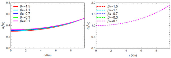
Figure 1.
Profiles of the metric coefficients ‘’ and ‘’, with respect to the radial coordinate r.
5.2. Energy Density, Pressure, and Anisotropy
The density (), the radial pressure (), and the tangential pressure () must all be positive within the stellar interior, decreasing towards the boundary and finite at the core for a model to be considered stable. In addition, for the solution of the present model to be physically accepted, the radial pressure () must be zero at the boundary.
At the center of a star, the anisotropy becomes zero as both the radial pressure and the transversal pressure are equal at that point. That means , indicating that the center of a star exhibits an isotropic situation. Furthermore, the anisotropic force will be repulsive or attractive based on or . If the force is repulsive, the stellar body may expand, becoming larger and potentially less stable. Nuclear fusion reactions and the star’s entire life cycle may be affected by this expansion, which could lower the density and pressure at the core. On the flip side, a contraction induced by an attractive force increases the density and pressure of the stellar body. The formation of black holes or neutron stars may be the outcome of this contraction, which can intensify gravitational forces under extreme circumstances.
Figure 2 and Figure 3 demonstrate that the physical quantities () remain finite and feasible through the stellar radius; that is, no singularity occurs. The aforementioned figures also show that the radial pressure drops to zero at km, and the energy density and pressures decrease monotonically toward the boundary. The graph of the anisotropic factor with respect to the radial coordinate r, as presented in Figure 4, shows that for various values of . Thus, the anisotropic nature turns outward-directed and repulsive, and thereby the proposed model depicts a more huge and compact star configuration. The radially symmetric diagram for matter variables with is shown in Figure 5.
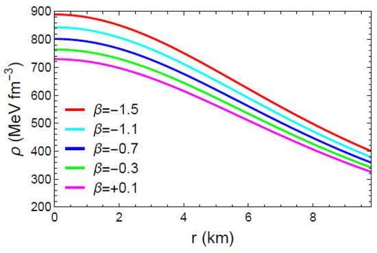
Figure 2.
Profile of the energy density () with respect to the radial coordinate r.
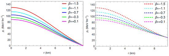
Figure 3.
Profile of the radial Pressure () (left) and tangential pressure () (right) w. r. t. the radial coordinate r.
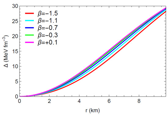
Figure 4.
Profile of the anisotropy w. r. t. the radial coordinate r.
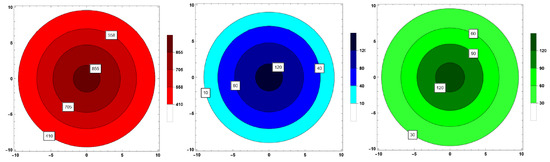
Figure 5.
Contour plots of energy density () (left), radial pressure () (middle) and tangential pressure () (right) with respect to the radial coordinate r corresponding to the compact star pulsar 4U1608-52 for = −1.5 respectively.
5.3. Equation of State Parameters
Determining the equation of state parameters (EoS) is an essential method to describe the relationship between pressure and density of matter. The EoS for the present model is defined by
The Zeldovich’s [47] requirement states that to maintain a physically feasible fluid arrangement, the value of the pressure density ratio must fall between 0 and 1.
Figure 6 displays the profiles of these two components () for various values of . As can be seen from the graphs, the radial and tangential components of the state parameters both monotonically decrease and fall between 0 and 1 throughout the matter distribution. Thus, in the case of our model, the EoS parameters met the physically correct conditions.
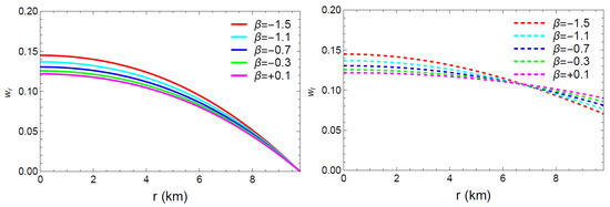
Figure 6.
Graphical representation of the ratio of state parameters () with respect to the radial coordinate ‘r’.
5.4. Gradients of Energy Density and Pressure
For being regarded as a viable model of an anisotropic compact star, the energy density and pressure should be maximum at the center with a monotonically decreasing trend over the stellar surface. That means
Figure 7, Figure 8 and Figure 9 show a graphical representation of the first order derivatives of , and . It is simple to infer from the figures that the energy density (), the radial pressure () and the tangential pressure () met the requirements of Equation (37) and reached their maximum value at the center of the celestial objects.
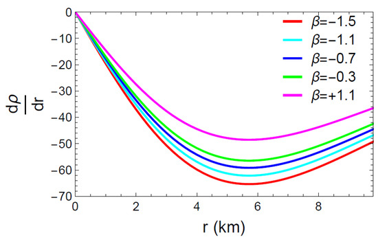
Figure 7.
Behavior of the derivative with respect to the radial coordinate r.
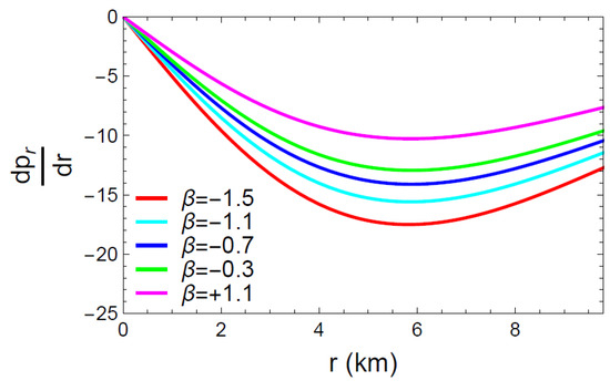
Figure 8.
Behavior of the derivative w.r.t. the radial coordinate r.
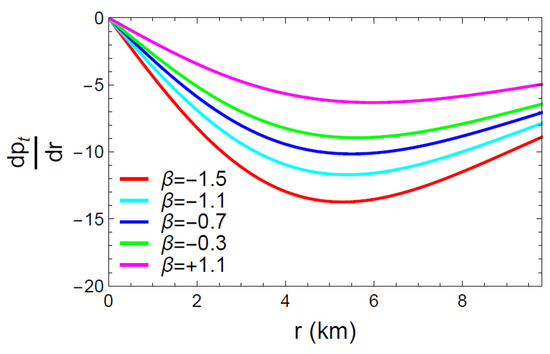
Figure 9.
Behavior of the derivative w.r.t. the radial coordinate r.
5.5. Energy Conditions
For being physically viable, the anisotropic fluid sphere composed of dense matter must be subjected to a set of constraints based on density and pressure known as energy conditions. There are different techniques for evaluating energy bounds, but in this study, the classification of these bounds is discussed as follows:
- Null Energy Condition (NEC): ;
- Weak Energy Condition (WEC): ;
- Strong Energy Condition (SEC): ;
- Trace Energy Condition (TEC): .
Figure 10 displays the left-hand side of the inequality of energy bounds versus r for the compact star pulsar 4U1608-52. According to the figure, the chosen star meets all the energy constraints, confirming the presence of a usual fluid configuration inside stellar structures, which implies the physical acceptability of the model.
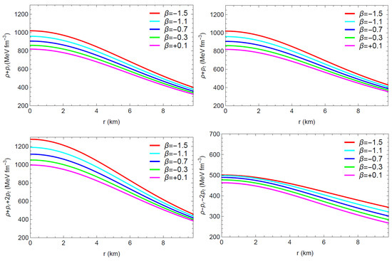
Figure 10.
Plots of energy conditions w.r.t. the radial coordinate ‘r’.
6. Stability Analysis
To examine realistic and reliable models of stellar structures, stability analysis is essential. Using various mathematical techniques, researchers can determine the precise parameters that determine whether the star remains stable or undergoes significant changes. In this section, the adiabatic index, the causality requirement, and the Herrera cracking criterion are used to assess the stability of the current model.
6.1. Adiabatic Index
For a given energy density and pressure (both radial and tangential), the stability of compact stars and the stiffness of the equation of state can be determined using the adiabatic index (). According to Heintzmann and Hillebrandt [48], the adiabatic index () value for a dynamically stable compact celestial object must be greater than over the entire inner area of the object. In contrast, if this is less than , the star will be unstable and might collapse due to its own gravity. There are a couple of techniques to define the adiabatic index for the suggested model, which are
- Radial adiabatic index: and tangential adiabatic index: .
Plots of these factors in Figure 11 reveal that, for the compact star pulsar 4U1608-52 with various values of the model parameter , and throughout the whole interior region. As a result, the model represents a dynamically stable stellar configuration.
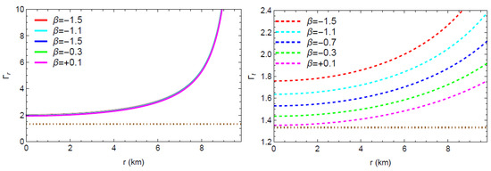
Figure 11.
Variations of adiabatic indices ( and ) w.r.t. the radial coordinate ‘r’.
6.2. Causality Requirement
In order to satisfy the causality constraint, the sound velocity within the compact object must be sub-luminal. A compact stellar structure must satisfy the causality requirements at every point throughout the entire interior region for the model to be physically accurate. The velocity of sound in an anisotropic stellar fluid, with (speed of light), is defined as
- Radial velocity: and tangential velocity: .
- From a mathematical point of view, the radial and tangential components of the sound velocity should meet the requirement that and .
Figure 12 exhibits the graphical behavior of and for the compact star model, pulsar 4U1608-52, with different values of . The figure confirms that both the graphs of radial and tangential components of sound velocity lie between 0 and 1 and monotonically decrease throughout the interior region. Therefore, it may be considered that the stellar solution satisfies the causality condition across the interior region.
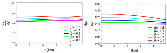
Figure 12.
Graphs of and with respect to the radial coordinate ‘r’.
6.3. Herrera Cracking Method
In order to investigate the stability of the anisotropic matter configuration, Herrera [49] developed the innovative idea of cracking (or overturning). According to the cracking concept, the radial velocity of sound exceeds the tangential velocity in a possibly stable region in the matter distribution. The theory also implies that the criterion must hold throughout the stable stellar interior, which assumes that there cannot be any cracking in that stellar structure. Furthermore, in order to figure out the potentially stable/unstable anisotropic compact object, Abren et al. [50] proposed a new range for Herrera’s cracking concept. According to their research, the following criterion determines that the star model inside the anisotropic matter configuration is possibly stable or unstable. for a potentially stable model and for a potentially unstable model.
Based on Figure 13, the inequality is satisfied, and thus Herrera’s cracking concept is inferred to be fulfilled by the present model. Consequently, it can be said that the model under consideration is physically stable.
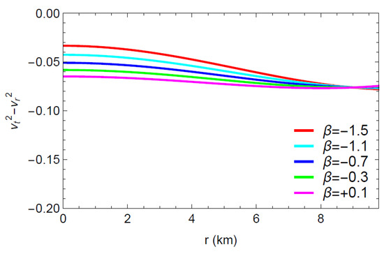
Figure 13.
Difference in sound velocities with respect to the radial coordinate ‘r’.
7. Equilibrium Through the Generalized TOV Equation
The Tolman–Oppenheimer–Volkhoff equation [51,52], or the TOV equation, is applied to examine whether the present model is in a hydrostatic state. The TOV equation in gravity with an anisotropic fluid configuration is defined as follows:
where , the effective gravitational mass can be obtained using the Tolman–Whittaker mass formula, which is as follows:.
Equation (38) yields the expressions as follows by applying the expression of :
The above equation can be rewritten in a simpler way as
where , , and represent the gravitational force, the hydrostatic force, and the anisotropic force, respectively.
The forces are expressed as follows:
Using the modified values for , and +0.1 as in the previous figures, the profiles of and for the present stellar model are shown in Figure 14. As seen in the figure, the condition of equilibrium for the system is amply justified by the reciprocal impact of the three forces and .
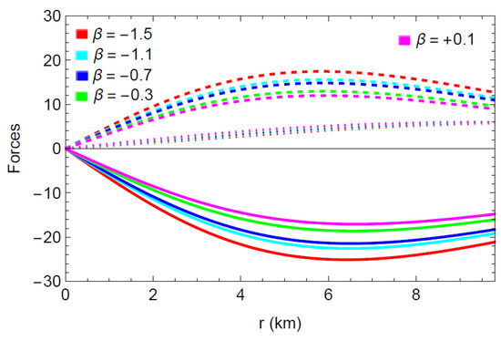
Figure 14.
Images of (plain curve), (dashed curve), and (dotted curve) with respect to the radial coordinate r for the compact star pulsar 4U1608-52 corresponding to the different values of .
8. Observations and Results
Predicting Einstein’s gravity variations inside of compact objects is merely natural. The development of massive objects under modified gravity theory has emerged as a central issue in relativistic astrophysics. gravity is a well-known modified theory that possesses many more significant properties than general relativity. In this article, an anisotropic uncharged compact stellar model is studied in the framework of gravity. An arbitrary linear function is considered to describe the framework of gravity with the formula , being an integrating constant. The Karmarkar condition is employed to get the exact solution for the field equation of the superdense compact stellar model by considering the Vaidya–Tikekar metric potential . The expressions for the model constants are determined by smooth matching of the interior solution with the Schwarzschild vacuum solution at the boundary of the stellar surface.
The present model is investigated graphically with respect to the compact star pulsar 4U1608-52 (mass and radius km) [53] and numerically in respect of the four compact stars KS1731-207, LMC X-4, Her X-1, and Cen X-3 at various levels. The model parameter emphasizes an important role in this investigation. According to the graphical analysis of the present model, a suitable range for , that is, , is determined to preserve the stability criterion of the anisotropic stellar structure.
Two instances of the graphical analysis can be expressed in the following manner.
Figure 15 shows that radial pressure vanishes at the boundary for but that acquires a positive value at the stellar boundary for . It is evident that the minimum value of is . Figure 16 exhibits that for and for . That justifies the fact that cannot be the maximum value of , whereas can be the largest value of .
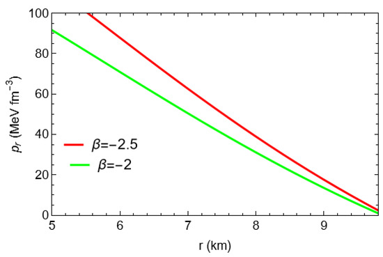
Figure 15.
Plots of radial pressure with respect to the radial coordinate ‘r’ for the compact star pulsar 4U1608-52 corresponding to and .
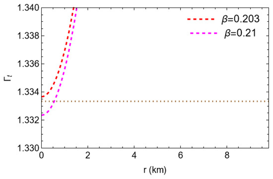
Figure 16.
Plots of tangential adiabatic index with respect to the radial coordinate ‘r’ for the compact star pulsar 4U1608-52 corresponding to and .
In order to test the model solution, five different values of are chosen within the range , such as , and . For the aforementioned known compact stars, Table 1 shows the values of the model constants that correlate with the various values, and Table 2 gives numerical data regarding the physical characteristics of the current model.

Table 1.
Model parameters and model constants that match many known compact stars.
Table 2.
Physical Features of the model corresponding to some known compact stars.
The final conclusions of the paper are summarized as follows:
In Figure 1, Figure 2 and Figure 3 and Figure 5, the metrices and the physical matter variables are investigated graphically. It seems that the metric potential is regular at the center and behaves nicely throughout the matter distribution. In the interiors of compact stars, the energy density , the radial pressure , and the tangential pressure are all positive, finite, and clearly defined. vanishes at the boundary of the star. The regularity of the matter variables () throughout the stellar structure is further supported by the contour plots in Figure 5. Most significantly, Figure 2 and Figure 3 and Table 2 provide evidence that the matter variables (, and ) gradually decrease as increases from negative to positive within the range of . Additionally, Figure 4 depicts that the anisotropy for the model grows throughout the stellar structure, providing a foundation for the stability of our model. Interestingly, within the intended range of , the anisotropy increases as increases.
- Figure 10 implies that the selected stars met all the energy requirements, indicating the presence of normal matter in the stellar interior of the present model.
- From Figure 11, Figure 12 and Figure 13 and Table 2, it can be seen that the adiabatic indices and , are both greater than within the stellar region. The radial and tangential sound velocity lie in the interval and the inequality holds for all selected compact stars at different levels. These suggest the physical stability of the proposed model.
- It is evident from Figure 14 that the combined influence of the hydrostatic and anisotropic forces balances the dominant gravitational force. Thus, the present model reaches the equilibrium state by the impact of three forces (). Consequently, the stability and conformity of the model with vital physical features indicates that the present anisotropic compact stellar object is considered physically acceptable.
Author Contributions
Conceptualization, S.D. and F.R.; Methodology, A.R.C.; Formal analysis, A.R.C. and S.D.; Investigation, F.R.; Writing—original draft, A.R.C.; Writing—review and editing, F.R.; Visualization, S.D.; Supervision, F.R. All authors have read and agreed to the published version of the manuscript.
Funding
This research received no external funding.
Data Availability Statement
No new data were created or analyzed in this study. Data sharing is not applicable to this article.
Acknowledgments
S.D. and F.R. express gratitude for the support from the Inter-University Center for Astronomy and Astrophysics (IUCAA), Pune, India, under its Visiting Research Associateship Program. S.D. would also like to thank ICARD, Malda College for providing support. F.R. is also thankful to ANRF, DST and DST FIST programme ( SR/FST/MS-II/2021/101(C)) for partial financial support respectively.
Conflicts of Interest
The authors declare no conflicts of interest.
References
- Schwarzschild, K. On the gravitational field of a mass point according to Einstein’s theory. Sitzungsber. Preuss. Akad. Wiss. Berlin (Math. Phys.) 1916, 1916, 189–196. [Google Scholar]
- Sotiriou, T.P.; Faraoni, V. f (R) theories of gravity. Rev. Mod. Phys. 2010, 82, 451. [Google Scholar] [CrossRef]
- Nojiri, S.I.; Odintsov, S.D. Gravity assisted dark energy dominance and cosmic acceleration. Phys. Lett. B 2004, 599, 137. [Google Scholar] [CrossRef]
- Hayashi, K.; Shirafuji, T. New general relativity. Phys. Rev. D 1979, 19, 3524. [Google Scholar] [CrossRef]
- Aldrovandi, R.; Pereira, J.G. Teleparallelism: A New Way to Think the Gravitational Interaction. Cienc. Hoje 2015, 55, 32. [Google Scholar]
- Maurya, S.K.; Errehymy, A.; Jasim, M.K.; Daoud, M.; AlHarbi, N.; AbdelAty, A.H. Complexity-free solution generated by gravitational decoupling for anisotropic self-gravitating star in symmetric teleparallel f (Q)-gravity theory. Eur. Phys. J. C 2023, 83, 317. [Google Scholar] [CrossRef]
- Aldrovandi, R.; Pereira, J.G. Teleparallel Gravity: An Introduction; Springer: New York, NY, USA, 2012; Volume 173. [Google Scholar]
- de Araujo, J.C.N.; Fortes, H.G.M. Mass of compact stars in f (T) gravity. Eur. Phys. J. C 2023, 83, 376. [Google Scholar] [CrossRef]
- Bamba, K.; Odintsov, S.D.; Sebastiani, L.; Zerbini, S. Finite-time future singularities in modified Gauss–Bonnet and F (R, G) gravity and singularity avoidance. Eur. Phys. J. C 2010, 67, 295. [Google Scholar] [CrossRef]
- Harko, T.; Lobo, F.S.N.; Nojiri, S.I.; Odintsov, S.D. f (R, T) gravity. Phys. Rev. D 2011, 84, 024020. [Google Scholar] [CrossRef]
- Xu, Y.; Li, G.; Harko, T.; Liang, S.D. f (Q, T) gravity. Eur. Phys. J. C 2019, 79, 708. [Google Scholar] [CrossRef]
- Nagpal, R.; Pacif, S.K.J.; Singh, J.K.; Bamba, K.; Beesham, A. Analysis with observational constraints in Λ-cosmology in f (R, T) gravity. Eur. Phys. J. C 2018, 78, 946. [Google Scholar] [CrossRef]
- Naseer, T.; Sharif, M.; Waqas, M.; Eid, M.R.; AbdelAty, A.H. Astrophysical stellar models in gravity under Tolman IV and Kohler-Chao-Tikekar spacetimes. Nucl. Phys. B 2025, 1020, 117146. [Google Scholar] [CrossRef]
- Shahzad, M.R.; Habib, W.; Noureen, I.; Ashraf, A.; Boukhris, I.; Alsaiari, N.S. Model of charged anisotropic compact sources in the framework of f (R, T) gravity. Eur. Phys. J. Plus 2025, 140, 691. [Google Scholar] [CrossRef]
- Ilyas, M. Compact stars in f (R, G, T) gravity. Int. J. Mod. Phys. A 2021, 36, 2150165. [Google Scholar] [CrossRef]
- Debnath, U. Constructions of f (R, G, T) gravity from some expansions of the universe. Int. J. Mod. Phys. A 2020, 35, 2050203. [Google Scholar] [CrossRef]
- Sharif, M.; Ikram, A. Energy Conditions in f (G, T) Gravity. Eur. Phys. J. C 2016, 76, 640. [Google Scholar] [CrossRef]
- Deb, D.; Rahaman, F.; Ray, S.; Guha, B.K. Strange stars in f (R, T) gravity. JCAP 2018, 2018, 44. [Google Scholar] [CrossRef]
- Das, K.P.; Debnath, U. Spherically symmetric anisotropic charged neutron stars in f (Q, T) gravity. Eur. Phys. J. C 2024, 84, 513. [Google Scholar] [CrossRef]
- Pradhan, S.; Mayura, S.K.; Sahoo, P.K.; Mustafa, G. Geometrically Deformed Charged Anisotropic Models in f (Q, T) Gravity. Fortschritte Phys. (Prog. Phys.) 2024, 72, 2400092. [Google Scholar] [CrossRef]
- Bhar, P. Charged strange star with Krori–Barua potential in f (R, T) gravity admitting Chaplygin equation of state. Eur. Phys. J. Plus 2020, 135, 757. [Google Scholar] [CrossRef]
- Zaman, U.; Ilyas, M.; Ahmed, I.; Khan, F. Modeling the structure and stability of compact stars in f (R, T) gravity using Tolman–Kuchowicz spacetime. Int. J. Geom. Meth. Mod. Phys. 2025, 34, 321. [Google Scholar] [CrossRef]
- Jeans, J. The Motions of Stars in a Kapteyn Universe. Mon. Not. R. Astron. Soc. 1922, 82, 122. [Google Scholar] [CrossRef]
- Weber, F. Strange quark matter and compact stars. Prog. Part. Nucl. Phys. 2005, 54, 193–288. [Google Scholar] [CrossRef]
- Sawyer, R.F. Condensed π—Phase in Neutron Star Matter. Phys. Rev. Lett. 1972, 29, 823. [Google Scholar] [CrossRef]
- Sokolov, A.I. Phase transition in a superfluid neutron liquid. Sov. Phys. JETP 1980, 79, 1137. [Google Scholar]
- Maurya, S.K.; Singh, K.N.; Govender, M.; Errerhymy, A. Anisotropic stars via embedding approach in Brans-Dicke gravity. Phys. Rev. D. 2019, 100, 044014. [Google Scholar] [CrossRef]
- Biswas, S.; Shee, D.; Guha, B.K.; Ray, S. Anisotropic strange star with Tolman–Kuchowicz metric under f (R, T) gravity. Eur. Phys. J. C. 2020, 80, 175. [Google Scholar] [CrossRef]
- Paul, B.C.; Deb, R. Relativistic solutions of anisotropic compact objects. Astrophys. Space Sci. 2014, 354, 421–430. [Google Scholar] [CrossRef]
- Bowers, R.L.; Liang, E.P.T. Anisotropic Spheres in General Relativity. Astrophys. J. 1974, 188, 657. [Google Scholar] [CrossRef]
- Karmarkar, K.R. Gravitational Matrices of Spherical Symmetry and Class One. Proc. Indian Acad. Sci. Sect. A 1948, 27, 56. [Google Scholar] [CrossRef]
- Sharif, M.; Gul, M.Z. Anisotropic compact stars with Karmarkar condition in energy-momentum squared gravity. Gen. Relativ. Gravit. 2022, 55, 10. [Google Scholar] [CrossRef]
- Nazeer, F.; Feroze, T. Karmarkar Bardeen anisotropic model for compact stars in gravity. Astrophys. Space Sci. 2025, 370, 33. [Google Scholar] [CrossRef]
- Wahid, S.; Mustafa, G.; Zubair, M.; Ashraf, A. Physically Acceptable Embedded Class-I Compact Stars in Modified Gravity with Karmarkar Condition. Symmetry 2020, 16, 962. [Google Scholar] [CrossRef]
- Maharaj, S.D.; Naidoo, N.; Amery, G.; Govinder, K.S. Lie group analysis of the general Karmarkar condition. Eur. Phys. J. C 2023, 83, 33. [Google Scholar] [CrossRef]
- Panday, D.M.; Thakore, B.; Goti, R.B.; Rank, J.P.; Shah, S. Anisotropic compact star model satisfying Karmarkar conditions. Astrophys. Space Sci. 2020, 365, 30. [Google Scholar] [CrossRef]
- Battista, E.; Capozziello, S.; Errehymy, A. Generalized uncertainty principle corrections in Rastall-Rainbow Casimir wormholes. Eur. Phys. J. C 2024, 84, 1314. [Google Scholar] [CrossRef]
- Naseer, T.; Sharif, M.; Fatima, A.; Manzoor, S. Constructing traversable wormhole solutions in f (R, Lm) theory. Chin. J. Phys. 2023, 86, 350–360. [Google Scholar] [CrossRef]
- Gul, M.Z.; Sharif, M. Spherically symmetric wormhole solutions admitting Karmarkar condition. Phys. Scr. 2024, 99, 055036. [Google Scholar] [CrossRef]
- Ospino, J.; Nunez, L.A. Karmarkar scalar condition. Eur. Phys. J. C 2020, 86, 166. [Google Scholar] [CrossRef]
- Vaidya, P.C.; Tikekar, R. Exact relativistic model for a superdense star. J. Astrophys. Astron. 1982, 3, 325–334. [Google Scholar] [CrossRef]
- Baskey, L.; Das, S.; Rahaman, F. An analytical anisotropic compact stellar model of embedding class I. Mod. Phys. Lett. A 2021, 36, 2150028. [Google Scholar] [CrossRef]
- Gauss, C.F. Disquisitiones Generales circa Supercies Curvas (General Investigations on Curved Surfaces). Comment. Soc. Regiæ Sci. Gottingensis Recent. 1827, VI, 99–146. [Google Scholar]
- Codazzi, D. Sulle coordinate curvilinee d’ una superficie e dello spazio. Ann. di Mat. 1868, 2, 269. [Google Scholar] [CrossRef]
- Pandey, S.N.; Sharma, S.P. Insufficiency of Karmarkar’s condition. Gen. Relativ. Gravit. 1981, 14, 113. [Google Scholar] [CrossRef]
- Birkhoff, G.D. Relativity and Modern Physics; Harvard University Press: Cambridge, UK, 1923; p. 253. [Google Scholar]
- Zeldovich, Y.B. The equation of state at ultrahigh densities and its relativistic limitations. Sov. Phys. JETP 1962, 14, 1143. [Google Scholar]
- Heintzmann, H.; Hillebrandt, W. Neutron stars with an anisotropic equation of state: Mass, redshift and stability. Astrophys. J. 1975, 38, 51–55. [Google Scholar]
- Herrera, L. Cracking of self-gravitating compact objects. Phys. Lett. A 1922, 165, 206–210. [Google Scholar] [CrossRef]
- Abreu, H.; Hernandez, H.; Nunez, L.A. Sound speeds, cracking and the stability of self-gravitating anisotropic compact objects. Class. Quant. Grav. 2007, 24, 4631. [Google Scholar] [CrossRef]
- Tolman, R.C. Static Solutions of Einstein’s Field Equations for Spheres of Fluid. Phys. Rev. 1939, 55, 364. [Google Scholar] [CrossRef]
- Oppenheimer, J.R.; Volkoff, G.M. On Massive Neutron Cores. Phys. Rev. 1939, 55, 374. [Google Scholar] [CrossRef]
- Ozel, F.; Psaltis, D.; Guver, T.; Baym, G.; Heinke, C.; Guillot, S. The dense matter equation of state from neutron star radius and mass measurements. Astrophys. J. 2016, 820, 28. [Google Scholar] [CrossRef]


Disclaimer/Publisher’s Note: The statements, opinions and data contained in all publications are solely those of the individual author(s) and contributor(s) and not of MDPI and/or the editor(s). MDPI and/or the editor(s) disclaim responsibility for any injury to people or property resulting from any ideas, methods, instructions or products referred to in the content. |
© 2025 by the authors. Licensee MDPI, Basel, Switzerland. This article is an open access article distributed under the terms and conditions of the Creative Commons Attribution (CC BY) license (https://creativecommons.org/licenses/by/4.0/).