1. Introduction
In recent years, biometrics has been studied as a method of authenticating people [
1], and modalities such as fingerprints and facial images have already been used in various applications. However, conventional biometrics is used in one time only authentication. Therefore, especially in user-management systems, conventional biometrics has the vulnerability that unregistered users can access the system after a registered user has logged in. An effective way to prevent this type of identity theft is to implement continuous authentication [
2,
3]. In continuous authentication, biometric data should be unconsciously presented because conscious presentation of biometric data would prevent the user from using the system. From a similar viewpoint, the password and ID card are also unsuitable for continuous authentication, while biometrics is more suitable.
Unconsciously presentable biometrics can be classified into two types. One is passively measured biometric data, such as the face and ears. However, biometric data of the face or the ear can easily be captured by using digital cameras. In other words, it is easy for others to steal biometric data while users are unaware of them being captured. As a result, fake faces or ears can be made by using captured data and then used for identity theft. The other type is biometrics that is detectable from the continuous actions of users, for example voiceprint in speaking, gait in walking, and keystrokes in typing. However, they are only usable in their actions; therefore, their applicable situations are limited. In conclusion, conventional biometric modalities are unsuitable for continuous authentication.
As a candidate of biometrics suitable for continuous authentication, brain waves measured by electroencephalography (EEG), which records electrical signals produced by an active human brain, are the focus. The signals are always produced as long as the person is alive, so this information can be continuously measured. Since brain waves are detectable only when the person is wearing a brain wave sensor, it is also not possible for others to covertly steal the data.
Using brain waves as biometrics has been actively studied [
4,
5,
6,
7,
8,
9,
10,
11,
12,
13,
14,
15,
16,
17,
18]. However, almost none of those studies have made mention of the applications. Using brain waves requires users to wear a brain wave sensor, but this takes time since users must set many electrodes on their scalp while moving their hair. It is not imaginable to do that when, for example, users enter a room, log in to a PC, or use an ATM. Therefore, brain waves as biometrics is not suitable for one time only authentication. On the other hand, once users wear a brain wave sensor in a continuous authentication environment, they are expected to work continuously for some time and will be focused on their work, becoming less conscious of wearing the sensor. In addition, as anyone can utilize brain waves, they are the most accessible biometric data. As a result, brain waves are the best for continuous authentication. However, it is accepted that wearing the brain wave sensor is an inconvenient process and takes time. Therefore, operator verification for high security systems is suitable for authentication using brain waves especially when the system is being used remotely by an assigned operator for some time [
19]. Operators are required to wear a brain wave sensor, and they are continuously verified while using the system. For instance, in a remote education system, students who are trying to obtain an academic degree or public qualification should be authenticated while learning. Operators of public transportation systems should be authenticated while operating the systems since hundreds of human lives depend on them. There are other examples: aircraft pilots, emergency vehicle drivers, and military weapon operators.
From that viewpoint, using brain waves as biometrics has been studied [
19,
20,
21,
22,
23,
24]. There are two types of brain waves: spontaneous brain waves that always occur and induced ones that are evoked by any thoughts or external stimuli. In [
19,
20,
21,
22,
23,
24], biometric authentication using spontaneous brain waves was studied, but the accuracy was not sufficient. Therefore, the uniqueness of induced brain waves when users are presented with stimuli is focused on here. However, since perceivable stimulation is a conscious activity for a user, it is unsuitable for continuous authentication. The stimuli must be unrecognizable to the user. Therefore, the acoustic sense, especially inaudible sounds, has been focused on [
25], and users were not distracted by this stimulation.
It has been proposed to use the stimulation for evoking some response in brain waves as biometrics, for example [
15,
26,
27] in a visual case and [
28] in an auditory case. However, all conventional approaches use perceivable stimulation.
2. Induced Brain Waves by Inaudible Sounds
The audible frequency range of human beings is generally from 20 Hz to 20 kHz, and sounds beyond 20 kHz are inaudible and called ultrasounds. However, it is known that such ultrasounds influence brain activity. For instance, analog record music has no frequency limitation; therefore, its sound quality was evaluated to be better than that of the compact disc, which has a frequency limitation of 22 kHz.
An evoked potential can occur when audible sounds are presented with ultrasounds [
29]. The
wave band (8–13 Hz) of brain waves is activated 20 s after the start of stimulus presentation. On the other hand, there is also a report that a similar phenomenon is only caused by ultrasounds [
30]. Therefore, it was necessary to investigate whether the phenomenon arose or not in an environment in this measurement. In the following, the abstract of the investigation is introduced, but for details, please refer to [
25] (in [
25], a surf sound was used, but it did not substantially include frequency elements beyond 20 kHz; therefore, it was removed, and re-evaluation was performed in this paper).
2.1. Making and Presenting Ultrasound Stimuli
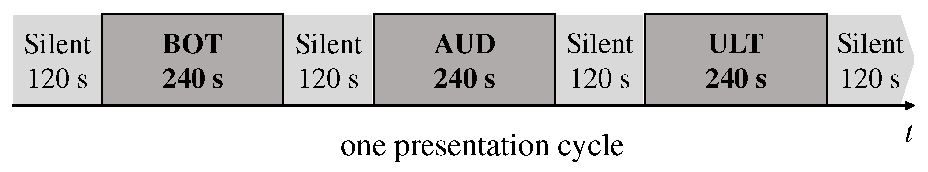
Four high resolution sounds were prepared that included ultrasounds, for which the sampling rate was 96 kHz and the bit depth was 24 bits. Ultrasound stimuli for 240 s were produced by filtering audible elements from high resolution sounds. For the sake of comparison, both audible and ultrasounds (BOT), only audible sound (AUD), and only an ultrasound (ULT) were presented in a presentation cycle, as shown in
Figure 1.
The reason why the interval of the presenting stimuli was 240 s was to take into account the phenomenon in which brain waves are activated 20 s after the start of stimulus presentation. It is also known that brain activity is maintained for approximately 100 s even after the end of stimulus presentation [
29]. In consideration of this, there was a silent interval of 120 s between stimulus presentations. However, the presentation order of the three stimuli was not random; therefore, its effect may not have been completely eliminated, even with inserting the long silent interval.
For presenting the ultrasound stimulation to the experiment subjects, the following general-purpose instruments that can deal with high resolution sounds were used: the amplifier was DS-DAC-10, produced by KORG Inc., and its frequency range was 10 Hz–40 kHz with ±1 dB precision; the speaker was GX-70HD ii, produced by ONKYO Corp. Japan, and its frequency range was 48 Hz–100 kHz.
2.2. Measurement of Induced Brain Waves
Measurement of brain waves was achieved by using five experiment subjects who were male students of Tottori University, Japan, did not have auditory abnormalities, and had had sufficient sleep. The measurement location was a room in Tottori University, and its quiescent state was kept as such as much as possible. The setup of the equipment in the room is shown in
Figure 2.
The produced auditory stimuli were output from a computer and presented to the experiment subjects through the amplifier and speaker. The distance between the speaker and the subjects was 2.0 m. Considering the straightness of ultrasound, the height of a speaker super tweeter was set to be equal to that of the subjects’ ear. A sound level meter was placed near the ear for adjusting the levels of the original high resolution sounds to approximately 70 dB. A recorder that could deal with high resolution sounds was also used to confirm after measurement that the ultrasound stimuli were actually presented. To prevent artifacts due to eye blinking or other movement, lights in the room were turned off, and the subjects were instructed to stay still and to close their eyes. The number of presentation cycles per subject was four.
The brain wave sensor was EPOC, produced by EMOTIVE, U.S.A, which is for commercial use, of which the sampling frequency was 128 Hz and the measurable frequency range was 0.16–43 Hz. It also had 14 electrodes based on the extended international 10–20 system as shown in
Figure 3.
Any physiological consequence of exposing subjects to inaudible sounds for an extended period of time was not reported in [
29,
30]. In this measurement, the inaudible sounds used were produced by filtering audible elements from high resolution sounds that had no physiological consequence on human beings and for which the level was approximately 70 dB, which was not an abnormal condition for listening to sounds.
2.3. Preprocessing of Measured Brain Waves
Since dedicated devices for presenting a stimulus and measuring brain waves were not used, their synchronization was not performed in this measurement. However, music player software for controlling the presentation of stimuli and software for controlling the brain wave sensor were installed in the same computer, and their operating times were simultaneously displayed on the computer. Thus, presentation of each stimulus always started after the start of measuring brain waves. Then, the display image where the operating times of both types of software were displayed was captured by a digital camera. After each measurement, the time–distance between operating times was calculated by using the captured image, and it was regarded as a time lag of synchronization. By subtracting the sampled data corresponding to the time lag from the initiation site of the measured EEG data, EEG synchronization with the stimulus presentation was achieved.
An EEG was measured as a variation of voltage at an electrode from the reference electrode of CMS or DRL in
Figure 3. Each EEG tended to have a trend and/or a ground bias. From each synchronized EEG, trend and/or bias were/was eliminated by using an approximate straight line that was obtained by using the least-squares method.
2.4. Analysis of Induced Brain Waves
According to [
29], the
wave band EEG increases in power 20 s post-stimuli on occipital channels. Thus, the
wave band at electrode O1 was focused on in the following.
In each preprocessed EEG, the sampled data (this was defined as one frame) were truncated for 2 s from the start, and then, their power spectrum was obtained using FFT with the Hamming window. This process was repeated sifting the frame with an overlap of 1 s in the sampled EEG data. Next, the total of the power spectral elements in the wave band was calculated in each frame. The difference between the two first frames was calculated, and it was approximated by using an exponential function , where A and B were constants. This process was repeated for the first two frames, then for the first three frames, and so on. As the number of frames increased, the exponential term B was obtained.
Comparing the absolute value of B with a threshold in each process, if the B was larger than the threshold, the power spectrum was regarded as increasing or decreasing. If the absolute value of B was smaller than the threshold, the power spectrum was regarded as unchanged. The threshold was empirically set to 0.001 in this evaluation. When the sign of the B was positive or negative, the power spectrum was regarded as increasing or decreasing, respectively. This process was performed while increasing the number of frames one by one up to 60 s. In each process, the numbers of increasing, decreasing, and unchanged cases were counted.
Results are shown in
Figure 4, where the vertical axis presents the number of cases and the horizontal axis presents the number of frames in each process. The total number of cases was 20 (5 subjects × 4 times). This figure indicates how the power spectrum in the
wave band varied with time after the start of stimulus presentation was increased. As a result, at 20 s, there were many cases where the power spectrum was increased, and it was confirmed that some response was only evoked by the ultrasound in the brain.
3. Verification Using Personal Ultrasound
A response in brain waves was confirmed to be evoked only by presenting ultrasounds, but it was not guaranteed that such a response contained sufficient individuality.
3.1. Personal Ultrasound
Stimuli that mean something to the person produce different evoked potentials compared with random stimuli [
31,
32]. In this section, we outline when sounds that meant something to the individuals were introduced in order to generate more individuality in the evoked responses. However, all research into personal sound stimuli has only used audible sound [
31,
32]. It is unknown what type of potential is evoked when personal stimuli are presented as ultrasounds. Therefore, EEGs of individuals when they were presented with personal ultrasound stimuli were examined. For this, memorable music for each individual was used. The memorable music was selected preventing duplicated selections by using a questionnaire with the experiment subjects.
The way of generating ultrasounds was equal to that in
Section 2.1. Examples of the memorable sound’s spectrum that were recorded near the subject’s ear are shown in
Figure 5. It was confirmed that ultrasonic components beyond 20 kHz were presented to the subjects. In addition, not only the amplitude, but also spectral distribution were different. Therefore, it was difficult to normalize the contained amounts of ultrasonic components in memorable sounds. The following evaluations included the effects of the different contained amounts.
The condition and environment for measuring EEGs were identical to those in the previous experiment. A presentation cycle is shown in
Figure 6. After a silent interval time of 30 s, a personal ultrasonic stimulus (P) was presented to each subject for 30 s, and then, an ultrasonic stimulus that was unrelated to the subject (U) and an ultrasonic stimulus that was common to all subjects (C) were sequentially presented, inserting a silent interval time of 120 s. The reasons why the interval time for stimulus presentation was 30 s and the silent interval time was 120 s are the same as the statements mentioned in
Section 2.1. As an ultrasonic stimulus that was unrelated to each subject, a personal ultrasound for the other subject was used supposing the spoofing attack. The common ultrasound to all subjects was orchestral music and used for the purpose of reference. The number of subjects was 10. Each subject underwent ten measurements, and the order of the three stimuli was changed for each measurement.
3.2. Preprocessing and Feature Extraction
By using the synchronization method mentioned in
Section 2.3, a section of data for the 30 s from the start to the end of each stimulus was extracted, and then, the trend and/or the bias were/was eliminated. After that, by using FFT, a power spectrum was calculated from the preprocessed EEG, and then, the spectral elements in the
wave band (8–13 Hz: 150 elements) and
wave band (13–30 Hz: 510 elements) were extracted as individual features.
3.3. Verification Performance
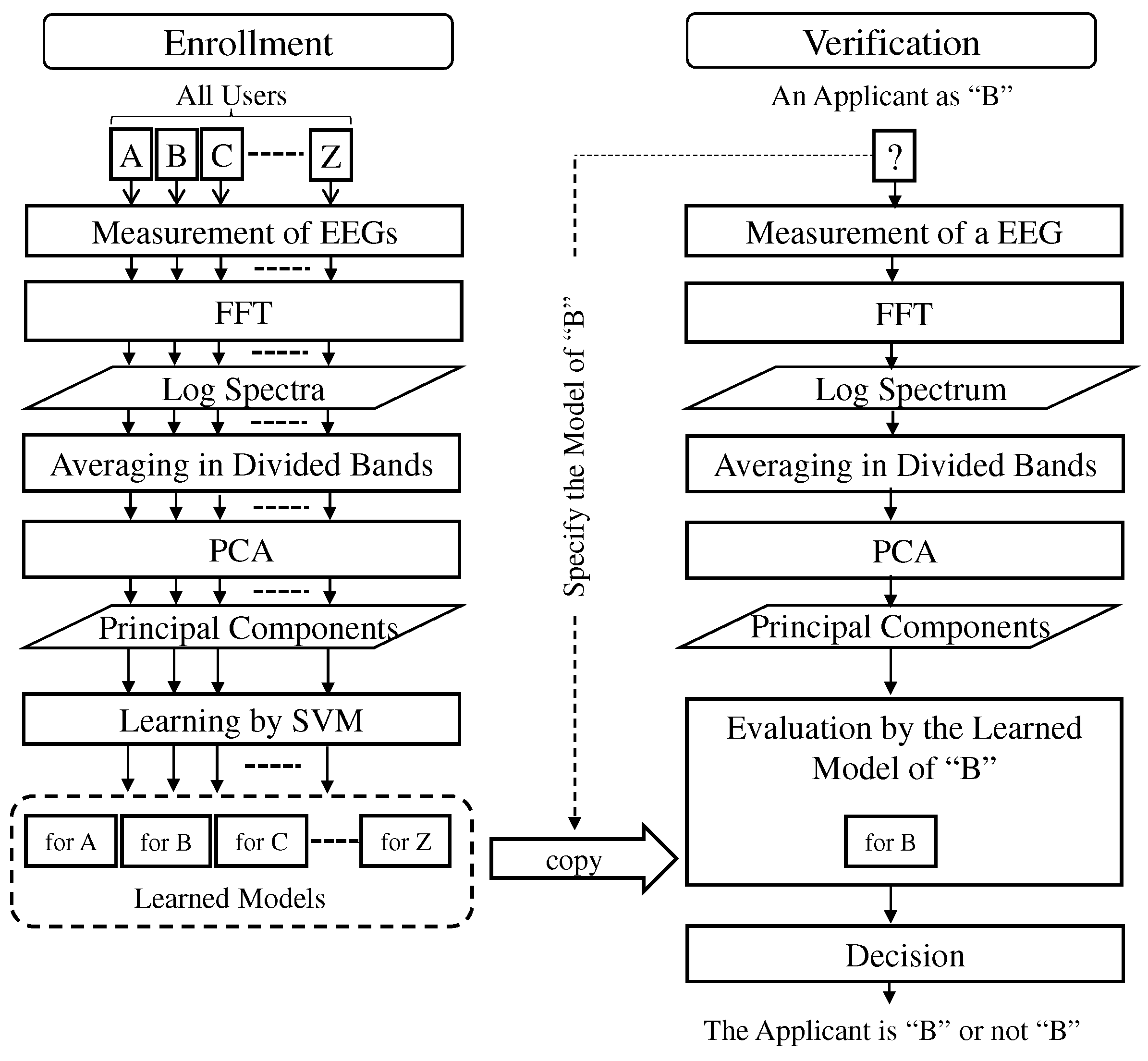
In this study, system-user verification was assumed. Verification was achieved by using Euclidean distance matching, and its procedure is shown in
Figure 7.
In the enrollment phase, EEGs were measured from all users, and then, their spectra in the
and
wave bands were obtained by FFT as individual features. To make a template, several EEGs of each subject were randomly chosen and then ensemble averaged. In the verification phase, an applicant who wanted to use the system specified for one of the enrolled users (for example, “A” in
Figure 7), his/her EEG was measured, and it was judged whether he/she was genuine based on Euclidean distance matching compared with the template relevant to the specified user. The obtained distance was compared with a threshold; then, if the distance was smaller than the threshold, the applicant was regarded as a genuine user. The threshold was empirically determined.
Measurements were performed ten times for each subject while changing an unrelated ultrasound in a presentation cycle, and as a result, for each subject, there were ten EEG data evoked by a personal ultrasound and ten EEG data evoked by nine unrelated ultrasounds (there were indeed two EEG data evoked by the same unrelated ultrasound for each subject). However, after measurement, abnormal EEG data caused by any measurement trouble were found (the measurement troubles did not happen on specified subjects and ultrasounds) and should be eliminated. In addition, the number of data for each subject should be equalized in evaluation. As a result, eight EEG data by a personal ultrasound and eight EEG data by unrelated ultrasounds were used as genuine data and imposter data, respectively, for each subject in this evaluation (The following concern may arise: There were unrelated sounds that were accordingly not used for a subject, and this might have an influence on the performance evaluation. However, the probability of eliminating abnormal EEG data was assumed quasi-random, and the cross-validation was achieved in this evaluation; therefore, their influence on performance evaluation was considered reduced.).
Among eight genuine data, four were used to make a template using ensemble averaging, and the remaining four were used in testing. Among eight imposter data, four were used in testing. However, this approach had a major disadvantage that, since only 50% of the dataset were used to make a template or in testing, there was a high possibility that some important information about the data might not be evaluated, and then, this would influence the verification performance. Therefore, to reduce the influence, cross-validation based on repeated random sub-sampling was introduced. Performance evaluation was conducted multiple times, and at each time, the data selection for making a template and imposter data was randomly changed. In other words, the subset of data were randomly sampled from the dataset. Verification performance was evaluated by averaging all results. In this evaluation, the number of random sub-sampling was 20.
In general, there are two error rates in an authentication system: a false acceptance rate (FAR), that is the rate of accepting imposters, and a false rejection rate (FRR), that is the rate of rejecting genuine users, were used, and there was trade-off between these error rates. The equal error rate (EER) where the FAR equals the FRR was used for the evaluation of authentication performance. A smaller EER showed a better performance.
Table 1 shows EERs when presenting personal ultrasounds (P) in the
and
wave bands for all electrodes and their averaged value compared with those when presenting the common ultrasound (C). From comparison of the averaged EERs, it was found that EERs when presenting the personal ultrasonic stimuli were smaller to those using the common one. This suggested that introducing the personal-ultrasound stimulation increased individuality in the evoked responses; therefore, verification performance was improved. However, the EER of around 40% was far from a satisfactory level.
4. Improvement of Verification Performance
In this section, several methods for improving the performance of the proposed verification method are introduced [
33].
4.1. Introduction of Log Spectrum
In the previous section, power spectra in the
and
wave bands were used as individual features. On the other hand, based on time frequency analysis using short time Fourier transform, an increase of the spectral content ratio was found at electrodes, especially in the front of the head, as shown in
Figure 8a, where the content ratio was the proportion of a power spectral element at each frequency bin to the sum of power spectral elements of all frequency bins. This phenomenon was not found in the case of unrelated stimulation, as shown in
Figure 8b.
However, in general, power spectral elements of the brain wave were localized in the
wave band (8–13 Hz), as shown in
Figure 9a, so there was a tendency that the variation of power spectral elements over 20 Hz was not reflected in the extraction of individual features. Therefore, a log spectrum was used where all frequency elements had logarithmic amplitudes, as shown in
Figure 9b. Higher frequency elements were emphasized, and this made it possible to reflect high frequency elements in the extraction of individual features.
In order to confirm the effect of using a log spectrum, verification performance using the log spectrum was compared with that by the conventional one. The verification method was Euclidean distance matching. Cross-validation was also performed.
Results are shown in
Table 2. EERs when using the log power spectrum (Lg) were slightly reduced compared with those when using power spectral elements (Sp). Considering the size of the database used, the differences might not be definitely significant. However, the log spectrum is commonly used for emphasizing high frequency elements, and its effect is confirmed in the field of signal processing; therefore, the log spectrum was also used in the following improvement steps.
4.2. Introduction of Support Vector Machine and Principal Component Analysis
For further performance improvement, an SVM was introduced into the verification procedure, which is shown in
Figure 10. SVMs are learning based two class classifiers that have the advantage of never having a local minimum, which is a weak point of neural networks [
34].
In the enrollment phase, EEGs were measured from all users (experiment subjects), and then, their log spectra (8–40 Hz, 960 dimensions) were obtained by FFT. However, the SVM tends to over-train when the number of dimensions is larger than that of the training data (in addition, fewer training times are useful in an authentication system). As mentioned in
Section 3.3, the number of training data per subject was a maximum of eight in this evaluation. Thus, to reduce the number of dimensions, the log power spectrum was divided into several partitions, and the average value was calculated in each partition. The number of partitions was empirically set to 24 in this evaluation (it was not confirmed whether 24 was the best). As a result, 40 average values were obtained. Furthermore, the average values were processed by PCA, in which the number of dimensions was reduced to three by extracting the top three principal components (the cumulative contribution of PCA was 80–90%), which were used as individual features. A one-vs.-all SVM model was trained to distinguish a user from others by teaching the SVM model to output
for genuine data and
for imposter data.
In the verification phase, an applicant specified a user (“B” in
Figure 10) and was judged by whether he/she was genuine by an SVM model relevant to the specified user. If the output of the SVM model was greater than a threshold, the applicant was regarded as a genuine user.
The EEG database obtained in the previous section was used. The number of genuine EEG data was eight, and the number of imposter EEG data was also eight. SVM is a two class method; therefore, it is better to equalize the number of data into two classes in training SVM models. Thus, when training each SVM model, four genuine data and four imposter data were used in training. The remaining data were used to evaluate the verification performance. To reduce the influence of selecting the data in learning and testing, cross-validation based on a random sampling method, which was introduced in
Section 3.3, was also used in this evaluation.
Tool kit
[
35], developed by Cornell University, was used to build the SVM models. To create an SVM model, it was necessary to set kernel functions and parameters. The cost parameter is a parameter that controls the trade-off between training error and model complexity. A too large parameter brings over-fitting, and a too small one brings under-fitting. The kernel function is to transform inseparable data into a space, where the transformed data becomes separable. In this evaluation, a polynomial function and a radial basis function (RBF) were used. The polynomial function had a parameter of
d, which defined the number of degrees. The RBF had a parameter of
, which defined a diameter of RBF. In general, these optimal values depend on a dataset; therefore, they were found with a grid search.
Table 3 shows the ranges of the parameters used in this evaluation.
Verification performance was evaluated where the number of random sampling for cross-validation was 10. EERs for all electrodes are shown in
Table 4. Their averaged value was 26.2% and greatly improved compared with 39.2% when using Euclidean distance matching. The effect of introducing PCA and SVM was notable, but further performance improvement was needed.
The best performance was EER = 22.0% for O2, and the EERs of O1 and O2 were relatively smaller than those of the others. O1 and O2 are located on the occipital lobe that mainly processes visual information. On the other hand, the EERs of electrodes O2, P8, T8, FC6, F4, F8, and AF4 in the right hemisphere were relatively smaller than O1, P7, T7, FC5, F3, F7, and AF3 in the left hemisphere. It is known that the right hemisphere is central for recognizing faces of known persons. Personal ultrasounds were also known to subjects. Such a condition might influence the above results, but further considerations are necessary.
4.3. Majority Decision Using Multiple Electrodes
EERs obtained by individual electrodes were inadequate. Therefore, multichannel judgment using the results from all electrodes was introduced. There are some approaches to fuse multiple modalities for authentication: input, feature, score, and decision level fusions. Between them, decision level fusion is easier to implement compared with the others. In decision level fusion, each modality is separately judged, and a final judgment is based on a logical operation of all judgment results. In this paper, decision level fusion was introduced into the decision stage in the verification procedure shown in
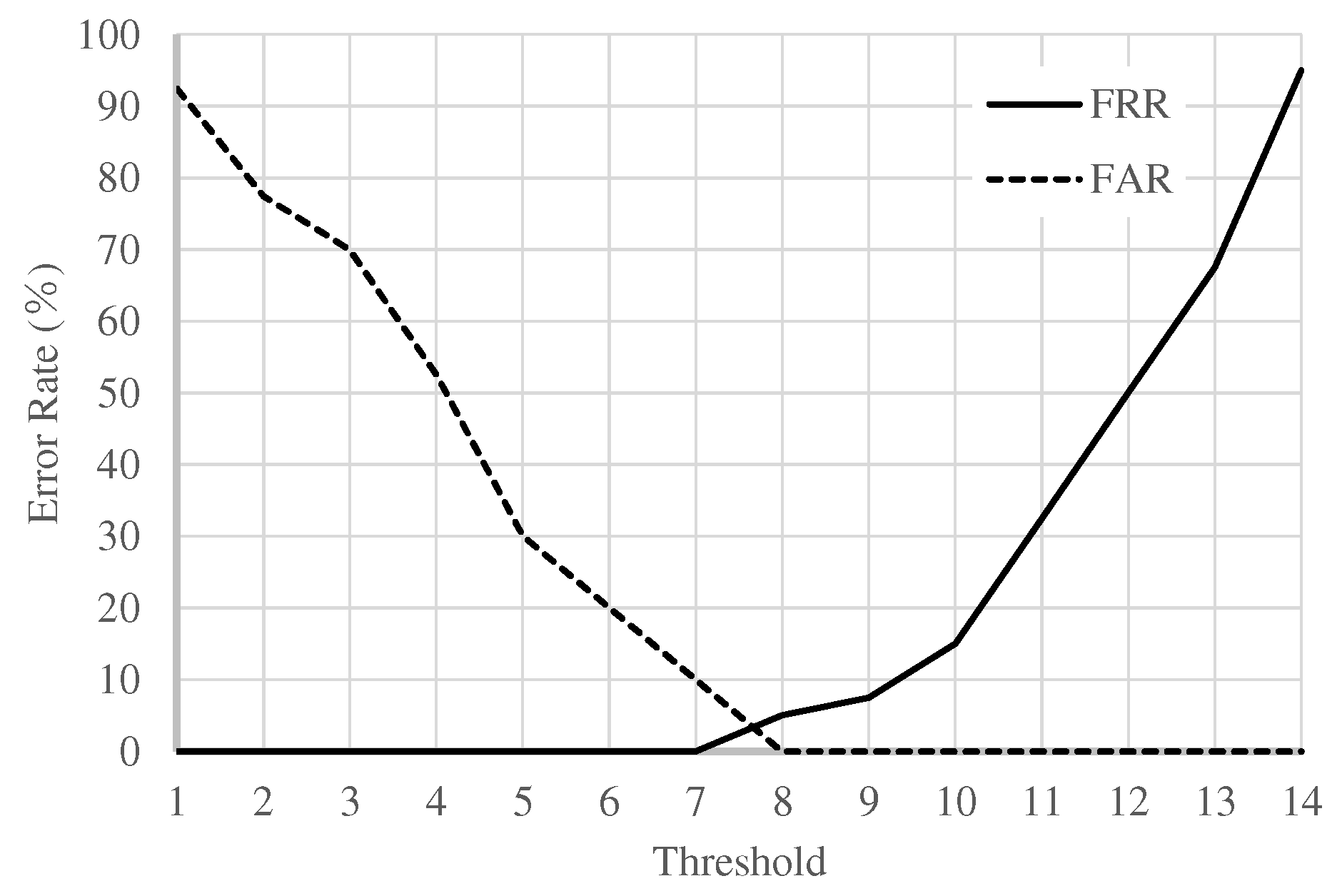
Figure 10. The most common verdict between the 14 electrodes (genuine or imposter) was adopted as the majority decision.
Figure 11 shows the error rate curves when using the majority decision rule. The value of the horizontal axis was a threshold, which was the number of electrodes (SVM models) needed to determine that the applicant was genuine based on the majority decision rule. As a result, the EER was 4.4%, which was dramatically improved compared with the EERs shown in
Table 4.
EERs were 5.9% and 11.0% when using the results from electrodes in the right hemisphere and the results from the top three electrodes, respectively; verification performance was not improved. In this case, robustness increased by using more electrodes, which might gain an advantage over accuracy improvement by selecting electrodes with better performance.
5. Introduction of Nonlinear Features
EERs using fingerprints as biometrics are less than 1%. Therefore, the EER of 4.4% in the previous section cannot be considered a great achievement. As a breakthrough, nonlinear analysis, especially chaos analysis, was introduced into feature extraction. The brain is a huge complicated system that consists of more than ten-billion neurons, and each neuron is connected to thousands or tens of thousands of other neurons. These activities are detected as electrical potential (EEG) on the scalp; therefore, it is not simple or linear. Chaos means the random and complicated behavior of a deterministic system. It is known that various phenomena in the natural world contain chaotic characteristics. The chaotic characteristics of biological signals have been studied [
36,
37] and have recently been utilized, for example, in autism assessment [
38] and in person authentication [
39].
5.1. Nonlinear Features Based on Chaos Analysis
In this paper, the maximum Lyapunov index, sample entropy, and permutation entropy based on chaos analysis were introduced as individual features. Please see the references cited in the following subsections for their definitions and estimation methods in detail.
5.1.1. Maximum Lyapunov Index
In chaos analysis, the maximum Lyapunov index indicates sensitivity to a system’s initial value. If a system shows a chaos characteristic, a delicate difference in initial value is exponentially propagated, thereafter having a large influence on the system. In a system with
k state variables, there are
k Lyapunov indices. If even one of them has a positive value, the system has sensitivity to an initial value. The maximum value of all the Lyapunov indices with a positive sign is called the maximum Lyapunov index. Using its amplitude and sign, sensitivity to the initial value can be evaluated. In this paper, Lyapunov indices were obtained using Takens’ embedding theorem [
40], and the maximum Lyapunov index was estimated using the Rosenstein method [
41].
5.1.2. Sample Entropy
A chaos system’s behavior is random and unpredictable, but never converges or diverges. Sample entropy is an index based on the regularity of a signal (sampled data) [
42]. As per chaos characteristics, small sample entropy indicates signal regularity, whereas large sample entropy indicates signal irregularity.
5.1.3. Permutation Entropy
Permutation entropy is an index based on the order of magnitudes of a signal [
43]. Similar to the case of sample entropy, a small value of permutation entropy indicates the low complexity of a signal, whereas large permutation entropy indicates the high complexity of a signal.
5.2. Parameter Determination
Before evaluating performance, the parameters of nonlinear features had to be determined. Generally, embedding delay for the maximum Lyapunov index is decided by the first local minimal value of the autocorrelation of an analyzed signal. In this evaluation, the first local minimal value from each EEG was obtained. Averaging the values obtained from all EEG data, was set to five.
The number of embedded dimension spaces
k for the maximum Lyapunov index was estimated using the false nearest neighbor method [
44], in which the embedded dimension space
k, which makes the number of false nearest neighbor zero, was regarded as optimum.
Figure 12 depicts the relationship between
k and the number of false nearest neighbors when
in this evaluation. As a result,
k was set to 4, where the number of false nearest neighbors asymptotically became zero.
The optimal parameters for sample entropy and permutation entropy were determined by trial and error by using Euclidean distance matching for verification. The reason for using the Euclidean distance matching method was its low computational cost.
6. Feature Multidimensionalization
Verification performance individually using the above mentioned nonlinear features was evaluated, but it was not improved. One of the reasons behind this was that the number of vectors in each nonlinear feature was only one. In this section, nonlinear features were fused to improve verification performance. Furthermore, extending nonlinear features in the time domain and the frequency domain was proposed. Finally, the extended nonlinear features were fused to the conventional spectral feature at the decision level.
6.1. Fusion of Nonlinear Features
First, the nonlinear features were fused. The simplest way to fuse features is to make a new feature that contains the original features as dimensions. Generally, each feature has a different variation range; therefore, in fusing several features, performing normalization is necessary to equalize them. However, the three above mentioned nonlinear features had an equivalent variation range; therefore, normalization was not introduced, and they were simply connected as a three-dimensional feature.
Results are presented in
Table 5, where the number of random samplings in cross-validation was 10. Mj represents the case of applying the majority decision to the results from all electrodes. The reduction of EERs for individual electrodes was not noticeable; however, the EER based on the majority decision was greatly reduced to 4.3%. On the other hand, little improvement was observed compared with the EER of 4.4% using the conventional spectrum feature in
Section 4.3.
6.2. Multidimensionalization of Nonlinear Features
To multidimensionalize, the above mentioned nonlinear features were proposed. In particular, the EEG was divided into several regions in the time domain or the frequency domain, and then nonlinear analysis was performed for each region. This resulted in the increase of the number of nonlinear features.
In the time domain, each EEG for 30 s was equally segmented without overlap, and a nonlinear feature was extracted from each segment. This was based on the assumption that the chaotic characteristic might vary with time. The time interval was discretionarily decided.
In the frequency domain, using a band pass filter bank, each EEG was divided into six signals, whose bandwidths were : 0.4–4 Hz, : 4–8 Hz, : 8–13 Hz, low : 13–20 Hz, high : 20–30 Hz, and : 30–43 Hz, and a nonlinear feature was extracted from each band.
There was no obvious criterion for the optimal time interval in the time domain extension and no knowledge about the optimal combination of a nonlinear feature and an extension method. Therefore, while changing the time interval and the combination, verification performance was evaluated using the Euclidean distance matching method in advance. For such a round-robin investigation, the Euclidean distance matching method, which has low computational cost, was suitable. As a result, the time interval and the combination with the best performance were decided as optimal.
Detailed results were omitted, but the best results were obtained when the sample entropy was combined with the time domain extension of eight segmentations, and permutation entropy was combined with the frequency domain extension. In the case of the maximum Lyapunov index, no great difference was observed between performances. Thus, the verification performance for the following four conditions was evaluated using PCA and SVM introduced in
Section 4.2.
- C1:
Maximum Lyapunov index and three time segmentations;
- C2:
maximum Lyapunov index and six frequency segmentations;
- C3:
sample entropy and eight time segmentations; and
- C4:
permutation entropy and six frequency segmentations.
The EERs for all electrodes and the EER fusing them based on the majority decision rule are presented in
Table 6. The electrodes with an even number were set on the right side of the brain, and those with odd numbers were set on the left side of the brain. It was found that the EERs for the electrodes set on the right side were smaller than EERs of the electrodes set on the left side of the brain. The right side of the brain controls the five senses of human beings, and the left side controls thinking; therefore, such a difference may be reflected in the above mentioned results.
Between the EERs based on the majority decision rule, the best performance of EER = 3.1% was obtained in the case of using the maximum Lyapunov index with frequency segmentation. Comparing with the conventional best result of EER = 4.4%, verification performance was observed to be slightly improved.
6.3. Fusion with Conventional Spectral Features
Finally, results obtained using the multidimensionalized nonlinear features were fused with those obtained using the conventional spectrum feature to further improve performance. As multidimensionalized nonlinear features, the maximum Lyapunov index in six frequency segmentations, sample entropy in eight time segmentations, and permutation entropy in six frequency segmentations were used. In particular, results for all electrodes in all features (14 × 4 = 56) were fused on the basis of the majority decision rule. The number of random samplings in the cross-validation was 10.
The error rate curves are illustrated in
Figure 13. Values in the horizontal axis correspond to the number of majorities, of which the maximum was 56. An EER of 0% was achieved in the end. However, 56 SVM models were needed, and the computational cost for making them was quite high. This was unrealistic from the viewpoint of computational time. Therefore, it was necessary to reduce the computational cost by selecting the electrodes used while maintaining verification performance.
6.4. Summary of Obtained Results
Figure 14 shows the summary of the results obtained in this paper. Nonlinear features, the maximum Lyapunov index, sample entropy, and permutation entropy were introduced, and fusion by combining three nonlinear features was evaluated. In addition, extension of nonlinear features in the time domain and the frequency domain was proposed and then evaluated. Finally, the decision level fusion of results by spectral features and extended nonlinear features were evaluated. As a result, an EER of 0% was achieved when the spectral features and extended nonlinear features were fused.
These results suggested which feature was not the most effective, feature multidimensionalization, especially fusion based on the majority decision rule, which was effective at improving performance.
7. Conclusions
The purpose of this study was to authenticate individuals using potentials evoked by ultrasound, which is never perceivable by human beings. In order to increase individuality in the evoked response, personal ultrasound stimuli were created using memorable sounds. A verification system using brain waves induced by personal stimulation was created, and its verification performance was evaluated. Features used in the proposed system were the log power spectrum and nonlinear features based on chaos analysis: the maximum Lyapunov index, sample entropy, and permutation entropy, and their extensions in the time domain and the frequency domain. As a result, by fusing the results of the extended nonlinear features and those of the spectral feature, an EER of 0% was achieved. This required high computational cost; therefore, it is not applicable to practical applications if the computational cost is not reduced. However, it was at least confirmed that person authentication using the induced brain waves by an inaudible sound was feasible.
Reducing the computational cost of the proposed method while keeping EER of 0% is now under research. Reducing the number of electrodes in fusing brings less computational cost. Using a more effective and smaller computational cost classifier than SVM is also a future work. Fractal dimension analysis is another nonlinear feature based on chaos. Future work will also introduce this as an individual feature and to evaluate its verification performance. In this paper, decision level fusion, in which the verdicts for all electrodes were integrated and the final verdict was the majority decision, was used. To further improve performance, feature level fusion and score level fusion will be considered. Furthermore, measuring the brain waves of more subjects is necessary to show the validity of the results obtained in this paper. Additionally, although memorable music to the users was used as the personal stimulus, it increased the risk of other users selecting the same piece of music when the number of users increased. Therefore, we considered using highly personalized stimuli, such as the person’s name.
Toward the practical use of the proposed method, some problems need to be overcome. A major one is artifacts in a brain wave due to eye blinking or other movement, which was restricted in this measurement. Many methods for reducing artifacts have been studied. By introducing some reduction method, the proposed approach can be evaluated in a more practical environment.
Author Contributions
Conceptualization, I.N.; methodology, I.N. and T.M.; software, T.M.; validation, I.N. and T.M.; formal analysis, I.N. and T.M.; investigation, I.N. and T.M.; resources, I.N.; data curation, T.M.; writing–original draft preparation, I.N.; writing–review and editing, I.N.; visualization, I.N. and T.M.; supervision, I.N.; project administration, I.N.; funding acquisition, I.N. All authors have read and agreed to the published version of the manuscript.
Funding
Part of this work was supported by KAKENHI (15K00184) in Japan.
Conflicts of Interest
The authors declare no conflict of interest.
References
- Jain, A.; Bolle, R.; Pankanti, S. BIOMETRICS Personal Identification; Kluwer Academic Publishers: Norwell, MA, USA, 1999. [Google Scholar]
- Altinok, A.; Turk, M. Temporal integration for continuous multimodal biometrics. In Proceedings of the 2003 Workshop on Multimodal User Authentication, Santa Barbara, CA, USA, 11–12 December 2003; pp. 207–214. [Google Scholar]
- Kwang, G.; Yap, R.H.C.; Sim, T.; Ramnath, R. An Usability Study of Continuous Biometrics Authentication; Tistarelli, M., Nixon, M.S., Eds.; ICB2009, LNCS5558; Springer: Berlin/Heidelberg, Germany, 2009; pp. 828–837. [Google Scholar]
- Poulos, M.; Rangoussi, M.; Chrissikopoulos, V.; Evangelou, A. Person identification based on parametric processing of the EEG. In Proceedings of the 9th IEEE International Conference on Electronics, Circuits and Systems, Pafos, Cyprus, 5–8 September 1999; Volume 1, pp. 283–286. [Google Scholar]
- Poulos, M.; Rangoussi, M.; Alexandris, N. Neural networks based person identification using EEG features. In Proceedings of the 1999 International Conference on Acoustic Speech and Signal Processing, Phoenix, AZ, USA, 15–19 March 1999; pp. 1117–1120. [Google Scholar]
- Poulos, M.; Rangoussi, M.; Chissikopoulus, V.; Evangelou, A. Parametric person identification from the EEG using computational geometry. In Proceedings of the 6th IEEE International Conference on Electronics, Circuits and Systems, Pafos, Cyprus, 5–8 September 1999; pp. 1005–1008. [Google Scholar]
- Paranjape, R.B.; Mahovsky, J.; Benedicent, L.; Koles, Z. The electroencephalogram as a biometric. In Proceedings of the 2001 Canadian Conference on Electrical and Computer Engineering, Toronto, ON, Canada, 13–16 May 2001; Volume 2, pp. 1363–1366. [Google Scholar]
- Ravi, K.V.R.; Palaniappan, R. Recognition individuals using their brain patterns. In Proceedings of the 3rd International Conference on Information Technology and Applications, Olympic City, Sydney, Australia, 4–7 July 2005. [Google Scholar]
- Palaniappan, R. Identifying individuality using mental task based brain computer interface. In Proceedings of the 3rd International Conference on Intelligent Sensing and Information Processing, Bangalore, India, 14–17 December 2005; pp. 239–242. [Google Scholar]
- Palaniappan, R. Multiple mental thought parametric classification: A new approach for individual identification. Int. J. Signal Process. 2005, 2, 222–225. [Google Scholar]
- Mohammadi, G.; Shoushtari, P.; Ardekani, B.M.; Shamsollahi, M.B. Person identification by using AR model for EEG signals. In Proceedings of the World Academy of Science, Engineering and Technology, Prague, Czech Republic, 24–26 February 2006; Volume 11, pp. 281–285. [Google Scholar]
- Palaniappan, R.; Ravi, K.V.R. Improving visual evoked potential feature classification for person recognition using PCA and normalization. Pattern Recognit. Lett. 2006, 27, 726–733. [Google Scholar] [CrossRef]
- Marcel, S.; Millan, J.R. Pearson authentication using brainwaves (EEG) and maximum a posteriori model adaption. IEEE Trans. Pattern Anal. Mach. Intell. 2007, 29, 743–748. [Google Scholar] [CrossRef]
- Palaniappan, R.; Mandic, D.P. Biometrics from brain electrical activity: A machine learning approach. IEEE Trans. Pattern Anal. Mach. Intell. 2007, 29, 738–742. [Google Scholar] [CrossRef]
- Singhal, G.K.; Ramkumar, P. Person identification using evoked potentials and peak matching. In Proceedings of the 2007 Biometric Symposium, Baltimore, MD, USA, 11–13 September 2007. [Google Scholar]
- Riera, A.; Soria-Frish, A.; Caparrini, M.; Grau, C.; Ruffini, G. Unobtrusive biometrics based on electroencephalogram analysis. EURASHIP J. Adv. Signal Process. 2007, 2008. [Google Scholar] [CrossRef]
- Pozo-Banos, M.D.; Alonso, J.B.; Ticay-Rivas, J.R.; Travieso, C.M. Electroencephalogram subject identification: A review. Expert Syst. Appl. 2014, 41, 6537–6554. [Google Scholar] [CrossRef]
- Thomas, K.P.; Vinod, A.P. EEG-based biometric authentication using gamma band power during rest state. Circ. Syst. Signal Process. 2018, 37, 277–289. [Google Scholar] [CrossRef]
- Nakanishi, I.; Ozaki, K.; Li, S. Evaluation of the Brain Wave as Biometrics in a Simulated Driving Environment. In Proceedings of the International Conference of the Biometrics Special Interest Group (BIOSIG2012), Darmstadt, Germany, 6–7 September 2012; pp. 351–361. [Google Scholar]
- Nakanishi, I.; Baba, S.; Miyamoto, C. EEG Based Biometric Authentication Using New Spectral Features. In Proceedings of the 2009 IEEE International Symposium on Intelligent Signal Processing and Communication Systems, Kanazawa, Japan, 7–9 January 2009; pp. 651–654. [Google Scholar]
- Nakanishi, I.; Miyamoto, C. On-demand biometric authentication of computer users using brain waves. In Networked Digital Technologies, Communications in Computer and Information Science (CCIS); Zavoral, F., Yaghob, J., Pichappan, P., El-Qawasmeh, E., Eds.; Springer: Berlin/Heidelberg, Germany, 2010; Volume 87, pp. 504–514. [Google Scholar]
- Nakanishi, I.; Miyamoto, C.; Li, S. Brain waves as biometrics in relaxed and mentally tasked conditions with eyes closed. Int. J. Biometrics 2012, 4, 357–372. [Google Scholar] [CrossRef]
- Nakanishi, I.; Ozaki, K.; Baba, S.; Li, S. Using brain waves as transparent biometrics for on-demand driver authentication. Int. J. Biometrics 2013, 5, 321–335. [Google Scholar] [CrossRef]
- Nakanishi, I.; Yoshikawa, T. Brain waves as unconscious biometrics towards continuous authentication—The effects of introducing PCA into feature extraction. In Proceedings of the 2015 IEEE International Symposium on Intelligent Signal Processing and Communication Systems, Nusa Dua, Indonesia, 9–12 November 2015; pp. 422–425. [Google Scholar]
- Maruoka, T.; Kambe, K.; Harada, H.; Nakanishi, I. A Study on evoked potential by inaudible auditory stimulation toward continuous biometric authentication. In Proceedings of the 2017 IEEE R10 Conference, Penang, Malaysia, 5–8 November 2017; pp. 1171–1174. [Google Scholar]
- Das, R.; Maiorana, E.; Rocca, D.L.; Campisi, P. EEG Biometrics for User Recognition Using Visually Evoked Potentials. In Proceedings of the 2015 International Conference of the Biometrics Special Interest Group, Darmstadt, Germany, 9–11 September 2015; pp. 303–310. [Google Scholar]
- Ruiz-Blondet, M.V.; Jin, Z.; Laszlo, S. CEREBRE: A Novel Method for Very High Accuracy Event-Related Potential Biometric Identification. IEEE Trans. Inf. Forensics Secur. 2016, 11, 1–12. [Google Scholar] [CrossRef]
- Seha, S.N.A.; Hatzinakos, D. Human recognition using transient auditory evoked potentials: A preliminary study. IET Biometrics 2018, 7, 242–250. [Google Scholar] [CrossRef]
- Oohashi, T.; Nishina, E.; Honda, M.; Yonekura, Y.; Fuwamoto, Y.; Kawai, N.; Maekawa, T.; Nakamura, S.; Hukuyama, H.; Shibasaki, H. Inaudible High-Frequency Sounds Affect Brain Activity: Hypersonic Effect. J. Neurophysiol. 2000, 83, 3548–3558. [Google Scholar] [CrossRef] [PubMed]
- Suo, Y.; Ishibashi, K.; Watanuki, S. Effects of Inaudible High-Frequency Sounds on Spontaneous Electroencephalogram. Jpn. J. Physiol. Anthropol. 2004, 9, 27–31. (In Japanese) [Google Scholar]
- Giudice, R.; Lechinger, J.; Wislowska, M.; Heib, D.P.J.; Hoedlmoser, K.; Schabus, M. Oscillatory brain responses to own names uttered by unfamiliar and familiar voices. Brain Res. 2014, 1591, 63–73. [Google Scholar] [CrossRef]
- Bauer, A.K.R.; Kreutz, G.; Herrmann, C.S. Individual Musical Tempo Preference Correlates with EEG Beta Rhythm. Psychophysiology 2015, 52, 600–604. [Google Scholar] [CrossRef]
- Nakanishi, I.; Maruoka, T. Biometric authentication using evoked potentials stimulated by personal ultrasound. In Proceedings of the 2019 42nd International Conference on Telecommunications and Signal Processing, Budapest, Hungary, 1–3 July 2019; pp. 365–368. [Google Scholar]
- Cristianini, N.; Shawe-Taylor, J. An Introduction to Support Vector Machines and Other Kernel-Based Learning Methods; Cambridge University Press: Cambridge, UK, 2000. [Google Scholar]
- Joachims, T. SVM-light Support Vector Machine. Available online: http://svmlight.joachims.org/ (accessed on 22 November 2019).
- Lake, D.E.; Richman, J.S.; Griffin, M.P.; Moorman, R.J. Sample entropy analysis of neonatal heart rate variability. Am. J. Physiol. Integr. Compar. Physiol. 2002, 283, 789–797. [Google Scholar] [CrossRef]
- Roerdink, M.; Hlavackova, P.; Vuillerme, N. Center-of-pressure regularity as a marker for attentional investment in postural control: A comparison between sitting and standing postures. Hum. Mov. Sci. 2011, 30, 203–212. [Google Scholar] [CrossRef]
- Kang, J.; Zhou, T.; Han, J.; Li, X. EEG-based multi-feature fusion assessment for autism. J. Clin. Neurosci. 2018, 56, 101–107. [Google Scholar] [CrossRef]
- Kang, J.; Jo, Y.C.; Kim, S. Electroencephalographic feature evaluation for improving personal authentication performance. Neurocomputing 2018, 287, 93–101. [Google Scholar] [CrossRef]
- Takens, F. Detecting strange attractors in turbulence. In Dynamical Systems and Turbulence, Warwick 1980; Lecture Notes in Mathematics; Springer: Berlin/Heidelberg, Germany, 1981; Volume 898. [Google Scholar]
- Rosenstein, M.T.; Collins, J.J.; Luca, C.J. A practical method for calculating largest Lyapunov exponents from small data sets. Phys. D Nonlinear Phenom. 1993, 65, 117–134. [Google Scholar] [CrossRef]
- Richiman, J.S.; Lechinger, J. Physiological time-series analysis using approximate entropy and sample entropy. Am. J. Physiol. 2000, 278, 2039–2049. [Google Scholar] [CrossRef]
- Bandt, C.; Pompe, B. Permutation entropy—A natural complexity measure for time series. Phys. Rev. Lett. 2002, 88, 174102. [Google Scholar] [CrossRef] [PubMed]
- Kennel, M.B.; Brown, R.; Abarbanel, H.D.I. Determining embedding dimension for phase-space reconstruction using a geometrical construction. Phys. Rev. A 1992, 45, 3403–3411. [Google Scholar] [CrossRef] [PubMed]
Figure 1.
Presentation cycle of auditory stimulation (1). BOT, both audible and ultrasounds; AUD, only audible sound; ULT, only an ultrasound.
Figure 1.
Presentation cycle of auditory stimulation (1). BOT, both audible and ultrasounds; AUD, only audible sound; ULT, only an ultrasound.
Figure 2.
Measurement environment.
Figure 2.
Measurement environment.
Figure 3.
Electrode position.
Figure 3.
Electrode position.
Figure 4.
Variation of the power spectrum in the wave band when ultrasonic sound is presented.
Figure 4.
Variation of the power spectrum in the wave band when ultrasonic sound is presented.
Figure 5.
Examples of different inclusion properties of ultrasonic components in recorded sounds.
Figure 5.
Examples of different inclusion properties of ultrasonic components in recorded sounds.
Figure 6.
Presentation cycle of auditory stimulation (2). P, personal ultrasonic stimulus; U, ultrasonic stimulus that was unrelated to the subject; C, ultrasonic stimulus that was common to all subjects.
Figure 6.
Presentation cycle of auditory stimulation (2). P, personal ultrasonic stimulus; U, ultrasonic stimulus that was unrelated to the subject; C, ultrasonic stimulus that was common to all subjects.
Figure 7.
Verification procedure using Euclidean distance matching.
Figure 7.
Verification procedure using Euclidean distance matching.
Figure 8.
EEG power spectrograms when presenting (a) stimulus linked to an individual and (b) stimulus not linked to an individual.
Figure 8.
EEG power spectrograms when presenting (a) stimulus linked to an individual and (b) stimulus not linked to an individual.
Figure 9.
(a) EEG power spectrum and (b) its logarithmic spectrum.
Figure 9.
(a) EEG power spectrum and (b) its logarithmic spectrum.
Figure 10.
Verification procedure using support vector machine (SVM) and principal component analysis (PCA).
Figure 10.
Verification procedure using support vector machine (SVM) and principal component analysis (PCA).
Figure 11.
Error rate curves when using the majority decision rule.
Figure 11.
Error rate curves when using the majority decision rule.
Figure 12.
Relationship between k and the number of false nearest neighbors.
Figure 12.
Relationship between k and the number of false nearest neighbors.
Figure 13.
Error rate curves when fusing all features.
Figure 13.
Error rate curves when fusing all features.
Figure 14.
Summary of the obtained results.
Figure 14.
Summary of the obtained results.
Table 1.
Equal error rate (EER, %) when presenting personal ultrasounds.
Table 1.
Equal error rate (EER, %) when presenting personal ultrasounds.
| | AF3 | F7 | F3 | FC5 | T7 | P7 | O1 | O2 | P8 | T8 | FC6 | F4 | F8 | AF4 | Ave. |
|---|
| P | 43.0 | 41.6 | 40.0 | 40.6 | 43.4 | 43.3 | 41.8 | 42.9 | 40.7 | 40.2 | 41.0 | 39.6 | 44.6 | 42.3 | 41.8 |
| C | 45.5 | 45.0 | 44.7 | 45.4 | 46.2 | 45.4 | 42.1 | 43.4 | 44.0 | 46.8 | 42.6 | 43.5 | 47.1 | 43.9 | 44.7 |
| P | 43.8 | 41.9 | 42.9 | 42.2 | 46.9 | 45.6 | 40.7 | 40.5 | 42.4 | 39.2 | 41.2 | 38.2 | 45.3 | 42.5 | 42.4 |
| C | 48.5 | 46.5 | 48.2 | 48.3 | 48.8 | 47.3 | 41.6 | 43.1 | 43.4 | 46.3 | 44.2 | 43.9 | 44.8 | 43.1 | 45.6 |
Table 2.
EERs (%) when using the log power spectrum.
Table 2.
EERs (%) when using the log power spectrum.
| | AF3 | F7 | F3 | FC5 | T7 | P7 | O1 | O2 | P8 | T8 | FC6 | F4 | F8 | AF4 | Ave. |
|---|
| Sp | 45.1 | 45.1 | 43.0 | 45.8 | 49.6 | 42.3 | 38.5 | 38.7 | 40.5 | 40.8 | 37.4 | 40.7 | 46.7 | 39.6 | 42.3 |
| Lg | 41.5 | 40.4 | 42.2 | 46.1 | 44.7 | 42.2 | 34.3 | 30.8 | 38.4 | 36.6 | 37.3 | 36.9 | 43.0 | 35.0 | 39.2 |
Table 3.
Parameter ranges in grid searching.
Table 3.
Parameter ranges in grid searching.
| Cost parameter | 0.001, 0.002, ⋯, 0.009,
0.010, 0.015, ⋯, 0.095,
0.10, 0.15, ⋯, 0.95,
1.0, 2.0, ⋯, 9.0, 10.0 |
| Kernel function | Polynomial: d | 1, 2, 3 |
| RBF: | 0.001, 0.002, ⋯, 0.009,
0.010, 0.015, ⋯, 0.095,
0.10, 0.15, ⋯, 0.95,
1.0, 2.0, ⋯, 9.0, 10.0 |
Table 4.
EERs (%) when introducing SVM and PCA.
Table 4.
EERs (%) when introducing SVM and PCA.
| AF3 | F7 | F3 | FC5 | T7 | P7 | O1 | O2 | P8 | T8 | FC6 | F4 | F8 | AF4 |
|---|
| 26.5 | 30.8 | 26.5 | 32.0 | 32.0 | 26.8 | 22.6 | 22.0 | 24.9 | 25.2 | 23.6 | 25.9 | 25.2 | 22.3 |
Table 5.
EERs (%) when fusing nonlinear features. Mj, majority decision.
Table 5.
EERs (%) when fusing nonlinear features. Mj, majority decision.
| AF3 | F7 | F3 | FC5 | T7 | P7 | O1 | O2 | P8 | T8 | FC6 | F4 | F8 | AF4 | Mj |
|---|
| 26.3 | 30.7 | 27.9 | 28.1 | 27.5 | 25.6 | 28.3 | 26.3 | 27.2 | 24.4 | 32.9 | 27.4 | 31.0 | 26.2 | 4.3 |
Table 6.
EERs (%) in four conditions.
Table 6.
EERs (%) in four conditions.
| | AF3 | F7 | F3 | FC5 | T7 | P7 | O1 | O2 | P8 | T8 | FC6 | F4 | F8 | AF4 | Mj |
|---|
| C1 | 28.0 | 31.9 | 28.8 | 29.0 | 32.2 | 32.2 | 30.2 | 28.5 | 28.8 | 27.8 | 28.4 | 29.4 | 31.2 | 31.4 | 3.9 |
| C2 | 30.7 | 32.3 | 26.1 | 28.7 | 31.1 | 30.0 | 34.3 | 29.3 | 33.5 | 30.9 | 29.5 | 30.7 | 32.1 | 28.3 | 3.1 |
| C3 | 32.8 | 27.9 | 30.6 | 35.0 | 29.5 | 28.8 | 30.5 | 30.3 | 27.6 | 28.6 | 32.3 | 30.1 | 32.4 | 27.1 | 5.1 |
| C4 | 35.5 | 32.8 | 30.0 | 32.8 | 30.2 | 27.1 | 29.7 | 29.0 | 34.3 | 29.3 | 31.2 | 32.8 | 30.0 | 32.1 | 4.3 |
© 2019 by the authors. Licensee MDPI, Basel, Switzerland. This article is an open access article distributed under the terms and conditions of the Creative Commons Attribution (CC BY) license (http://creativecommons.org/licenses/by/4.0/).


