Abstract
Chaos through-wall imaging radar has attracted wide attention due to its inherent low probability of detection/interception, strong anti-jamming, and high resolution. However, the target response is usually overwhelmed by strong clutter. This paper proposes an imaging-then-decomposition method based on two-stage robust principal component analysis (RPCA) to remove the clutter and recover the target image. The proposed method firstly focuses the energy of the preprocessing data by the back-projection imaging algorithm; then, it performs matrix decomposition on the full and the sparse component of the focused data, in succession, by the RPCA algorithm. Simulation and experimental results show that the proposed method can suppress the clutter dramatically and indicate human targets distinctly. Compared with the traditional methods, it has effectiveness and superiority in improving the signal-to-clutter ratio.
1. Introduction
Through-wall imaging (TWI) radar plays an important role in both military and civil applications, such as urban warfare, antiterrorism, homeland security, law enforcement, and disaster survivor detection [1]. According to radar architecture, existing TWI radar systems can be classified into five types: continuous-wave radar, impulse radar, frequency-modulated continuous-wave radar, stepped-frequency continuous-wave radar, and random noise radar. Among these, random noise TWI radar has attracted increasing attention due to its inherent unambiguous high-resolution performance, low probability of detection/interception, and good anti-jamming ability [2,3,4]. Chaotic signal is noise-like but deterministic in nonlinear dynamical systems. Compared with the random noise signal, a wideband chaotic signal with large amplitude can be easily generated by simple nonlinear dynamical systems. Moreover, unlike noise, the chaotic signal is deterministic in that it is controllable and offers the possibility of synchronization [5,6]. Extensive studies have demonstrated that chaos TWI radar, which transmits a chaotic signal directly or chaos-based amplitude/frequency/phase modulated signal, has good range-Doppler resolution, excellent sidelobe suppression, and anti-jamming performance [7,8,9,10]. However, similar to other TWI radars, the human echo is usually overwhelmed by strong clutter because of its complex environment, wall attenuation, multipath reflection, unnecessary interference, and low reflectivity of the human body [11,12,13,14,15,16,17].
In order to obtain the image of a human target, typically, clutter suppression methods (time-domain methods, frequency-domain methods, and subspace-based techniques) are used firstly, and then the imaging algorithm is applied. At present, there are many methods for clutter suppression. Among them, the simplest but effective method is background subtraction [17], which subtracts the complex data without a target from that with the target to suppress the clutter, especially the wall clutter. However, it is not realistic to collect background data in many practical applications. The time window threshold method is intuitive, but its performance depends on the choice of time window, which is difficult to select. The spatial filtering method [18] removes zero-frequency or low spatial frequencies through the notch filter to suppress the clutter. It is effective when the wall is homogeneous and array apertures are perfectly parallel to the wall surface; however, it may not work for walls with spatially varying characteristics or misaligned antenna arrays. Subspace-based techniques [14,15,16,19], such as singular value decomposition (SVD), principal component analysis (PCA), and independent component analysis (ICA), which decompose raw data into subspaces corresponding to the clutter and the target components based on the strength difference between the clutter and the target reflection, but their performances rely on the selection of noise components. However, the target components may also contain wall clutter residual due to the interrelationships between the wall and nearby targets, and the multiple targets may not be represented by a single component. Besides that, these methods work ineffectively in heavy clutter environments.
Recently, Wright et al. [20] proposed a robust principal component analysis (RPCA) method (also called low-rank and sparse representation or sparse and low-rank decomposition) and showed that under rather broad conditions, the method can recover a low-rank matrix or a sparse matrix from highly corrupted measurements via decomposition. It has been demonstrated that RPCA is an effective clutter removal method in through-wall imaging applications [21,22,23,24]. For TWI radar, as the number of human targets is usually limited, the target responses are contained in a sparse matrix, and the clutters form a low-rank matrix. Therefore, RPCA can separate human targets and the background clutter, even in highly corrupted conditions. Zhang et al. [21] used RPCA to detect targets behind a reinforced concrete wall and proved that the clutter can be dramatically suppressed to improve the target detection performance. Tang et al. [22] presented a joint low-rank and sparsity-based method for compressed sensing TWI radar, which can mitigate the wall reflection and reconstruct an image of the scene even when the number of measurements is significantly reduced. Later, they proposed a low-rank and sparse imaging model to combine wall clutter mitigation with image formation for multipolarization TWI radar and verified its effectivity in removing unwanted wall clutter and enhancing the stationary targets under considerable reduction in measurements [23]. Qiu et al. [24] applied the RPCA method to micromotion human indication in UWB through-wall radar, and verified that the method can remove most of the clutter and avoid introducing extra ringing artifacts. Similarly, RPCA has also been widely used in ground penetrating radar (GPR) applications [24,25,26,27]. In [27], an improved clutter removal method that combines migration with RPCA was proposed in GPR detection of antipersonnel mines. Robust nonnegative matrix factorization (RNMF) [28] was also proposed recently for GPR detection, which is quite similar to the RPCA, but the low-rank and sparse decomposition algorithm is different.
For chaos TWI radar, target information cannot be obtained directly from the echo signal due to the randomness of the chaotic signal [9,10]. Cross-correlation between the echo signal and the reference signal is necessary to determine the position of the reflection events, which results in the target reflections appearing as wide and flat hyperbolas, which are sometimes nearly straight lines. In this case, the direct RPCA method performs insufficiently due to the degradation of the sparsity of the target responses.
In this paper, motivated by the success of the RPCA, an imaging-then-decomposition clutter suppression method based on two-stage RPCA is proposed for chaos TWI radar. Instead of using RPCA directly, it firstly enhances the sparsity of the cross-correlation data by the back-projection (BP) imaging algorithm and then extracts the target from the focused image by using RPCA twice. Unlike [27], where RPCA is used once with a general regularization parameter, the proposed method applies RPCA twice and optimizes the regularization parameter to balance the low-rank and sparsity components and to enhance the target detection performance for chaos TWI radar. Besides that, the layered range migration algorithm is used to focus the raw data in [22], while the proposed method adopts the back-projection method to enhance the correlation data.
The remainder of this paper is organized as follows. Section 2 introduces the principle of the conventional RPCA method. The proposed novel clutter removal method for chaos TWI radar is elaborated in Section 3. Numerical simulation and experimental demonstrations are presented in Section 4. Finally, Section 5 offers some conclusions.
2. Principle of the RPCA
The robust principal component analysis is proposed to recover corrupted low-rank data. Compared to classical PCA, it can effectively deal with incomplete or missing data suffering greater corruption; thus, it is attractive in practical applications. Note that in different cases, the object of interest could be in either a low-rank component or sparse component.
Mathematically, it decomposes the observed data matrix into a superposition of a low-rank matrix and a sparse matrix , where m is the number of sampling points and n is the number of scanning positions. The mathematical expression is D = L + S. Through Lagrangian reformulation, we can obtain the low-rank and sparse matrices by solving the following convex optimization problem:
where λ is a positive regularization parameter to control the tradeoff between the two components, and is the number of non-zero entries of a matrix. Unfortunately, the rank (L) and are both nonlinear and non-convex in Equation (1). To solve this NP-hard problem, a relaxed optimization model is presented by replacing the rank minimization with nuclear norm minimization and the l0-norm penalty with an l1-norm penalty [20]:
where is the sum of the singular values of the matrix, is the sum of the absolute values of the matrix entries, and λ universally equals 1/(max(m, n))1/2. It has been proven in [20] that under surprisingly broad conditions, exact recovery of the low-rank and the sparse components can be achieved by Equation (2), provided that the rank of the low-rank component is not too large and the sparse component is reasonably sparse, which can be described as follows:
where , are some positive constants and µ is a parameter related to the incoherence conditions on left- and right-singular vectors of L. According to [29], if are sufficiently small numerical constants, the decomposition can be more exact with high probability. It is worth noting that many variants of Equation (2) have been proposed with the goal being either lower complexity or better performance, but we just use the original one, since we focus on the utilization of the RPCA-based method in chaos TWI radar. Besides that, there are many algorithms for solving Equation (2), and we adopt the inexact augmented Lagrange multiplier (IALM) method [30] because it is easy to implement with high accuracy, fast computation speed, and less storage requirement.
3. A Proposed Novel Clutter Removal Method for Chaos TWI Radar
Consider a monostatic synthetic aperture radar for imaging targets behind the wall. Figure 1 depicts a through-wall imaging geometry, where the radar signal propagates through the air–wall–air interfaces. The wall with a thickness of d is non-magnetic and homogeneous. The wall plane is the (x,z) plane, and the down range is along the positive y axis. We assume that the transmitting (TX) and receiving (RX) antennas with a fixed separation cling to the wall, and they are both moved horizontally along a straight line with a fixed step size to synthesize an N-element linear antenna array. The target is located in the imaging area. At each scanning position, a wideband chaotic signal is transmitted, and an echo signal from the scene is received. Meanwhile, the reference signal, which is the replica of the transmitting signal, is also collected.
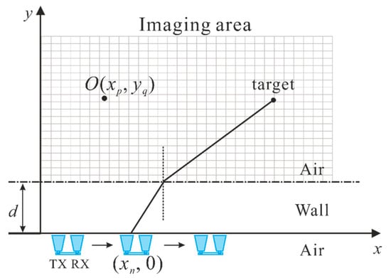
Figure 1.
A schematic diagram of a through-wall imaging scene.
Let denote the echo signal at the nth scanning position, which can be simply modeled as the superposition of the clutter and the target response :
The clutter can be caused by the wall reflections (including the reflections from the front surface and the back surface of the wall), the direct coupling between TX and RX (including antenna internal reflections), and the scattering response from non-target objects in the background [31]. Among these, wall reflection is dominant.
For the chaos TWI radar, the echo signal should be cross-correlated with the reference signal at each scanning position to obtain the target range. The cross-correlation function between them is as follows
where T represents the cross-correlation integral time, and τ is the delay time of the echo signal relative to the reference signal. Due to the natural characteristic of the chaotic signal, the cross-correlation result exhibits a delta-like profile, and the position of the correlation peak corresponds to the target range.
Upon the discretizing time, the echo signal and the reference signal at the nth observation position can be represented as and , respectively, where and is the number of sampling points; then, the cross-correlation result can be recorded as , where .
After cross-correlation, the Hilbert transform is applied to calculate the instantaneous amplitude of the cross-correlation signal. The mathematical expression is:
where denotes Hilbert transformation.
Since the cross-correlation and Hilbert transform are linear operations and do not change the low-rank and the sparse structures of the echo signal, the signal at the nth scanning position can also be modeled as
where is the low-rank background clutter and is the reflection signal from the target after the wall.
Denote , , and as (2M − 1) × 1 vectors , , and , respectively. Assembling the data of all the N scanning positions leads to the following (2M − 1)×N matrices
In the conventional method, firstly, the target reflection S is solved by Equation (2); then an imaging algorithm is used to obtain a two-dimensional image. However, we find that the performance of clutter removal is inadequate, since the target response in the cross-correlation matrix D often presents a wide and flat hyperbola signature that violates the sparsity constraint to some extent. According to [29], improving the sparsity of the sparse component will generally lead to a better decomposition. Therefore, we propose an imaging-then-decomposition method based on two-stage RPCA, which uses a prior BP imaging algorithm to enhance the sparsity of the target response and then applies RPCA twice to suppress the clutter.
The BP imaging algorithm is actually a delay-and-sum beamforming algorithm, which is the most popular and least complex imaging method for TWI radar [32,33]. The idea of this imaging algorithm is to sum all of the data coherently at each pixel point at a time and repeat for all of the points in the region. During the imaging, the pixel point moves from one position to another within the whole imaging region. As all of the time-shifted responses are coherently summed and integrated at each position, the hyperbola signatures of targets are focused, while the clutter maintain their original positions. Therefore, the sparsity of the target response is improved, and the low-rank property of the clutter remains unchanged. Moreover, the coherent imaging enhances the strength of the target response, which is beneficial to identify the target.
Suppose that the target area is divided into P×Q pixels, and O is a pixel in the imaging area located at , as shown in Figure 1. The amplitude of the pixel point O is the sum of the signals corresponding to the echo signals at different delay times. The mathematical formula of the BP algorithm can be represented as
where represents the round-trip delay time from the nth scanning position to the pixel point . Ignoring the wall effect, it can be simply obtained by
where c is the speed of light. The above equation can be revised according to [32] if considering the propagation delay through the wall.
The process, which is described by Equations (9) and (10), is performed for all the pixels in the imaging area to generate a whole image with a size of P×Q. For clarity, we give the detailed steps for BP in the discrete form.
Step (1): Construct an imaging area with a size of P×Q.
Step (2): Calculate the round-trip delay time by Equation (10).
Step (3): Calculate the amplitude of a pixel corresponding to a scanning position. According to the delay time , we can find the amplitude of the pixel in . However, the round-trip delay time usually does not coincide with the sampling points of , so linear interpolation should be used to obtain an approximation one.
where interp() means the linear interpolation method.
Step (4): Sum all the amplitudes corresponding to the N scanning positions for the pixel.
Step (5): Repeat Steps (2) to (4) for all pixels to form a whole image M.
From Equation (9), we can find that if the target is located at the pixel point O, the signal amplitude at the corresponding scanning position is strong, which means that the energy at the point O is focused; while if there is no target at the pixel point O, the signal amplitude is very small after coherent superposition. Therefore, the sparsity of the matrix is greatly improved, which is conducive to further decomposition. Besides that, after BP imaging, the image size is dramatically smaller than the correlation data, which is beneficial to accelerate decomposition.
After the BP imaging algorithm, the RPCA can be used effectively. The matrix M can be modeled as
where L contains the low-rank background clutter component, and S represents the sparse target component. The matrix S can be obtained by solving Equation (2).
The regularization parameter λ controls the tradeoff between the low-rank component and the sparse component, and it greatly affects the decomposition result. As the value of λ decreases, more sparse component information (target) is included in S, and if it falls below a certain value, clutter and noise information is transferred along the target information; then, the S image will contain not only the target component, but also the low-rank clutter component. On the contrary, with the increasing of the value of λ, more low-rank component information (clutter and noise) is included in L, and when the value is too large, the matrix S has little target information, sometimes resulting in the disappearance of the weak target. Therefore, in our proposed method, the λ value is optimized according to image quality criterion rather than equaling 1/(max(m, n))1/2. It is just selected in one experiment and fixed for all the experiments.
Moreover, we use RPCA twice to enhance the clutter removal performance. For the first RPCA, we select a suitable regularization parameter λ1 with a relative small value to ensure that the very strong clutter is removed while the weak target remains. We called it the coarse decomposition. After the first RPCA, the target component is contained in the sparse matrix S, as well as the remained clutter component. According the principle of the RPCA, assume that the sparse matrix S is the observed matrix; then, it can be decomposed into the superposition of a low-rank matrix L’ and a sparse matrix S’. We called it the fine decomposition. Through coarse-to-fine decomposition, the matrix S’ corresponds to the target image with little clutter.
This two-stage RPCA is more efficient in real applications or heavy clutter environments because in these cases, the target reflection is very weak, and it is difficult to remove the clutter effectively while retaining the weak target. Usually, after the conventional RCPA decomposition (even with the optimized parameter), some ghosts will still exist. Our proposed method has a larger selection range of regularization parameters to balance the clutter and the target components for each decomposition, and then makes sure that there is a better clutter removal performance, which will be demonstrated in Section 4. The procedures of the proposed method (referred to as BP-RPCA2) are presented in Figure 2.
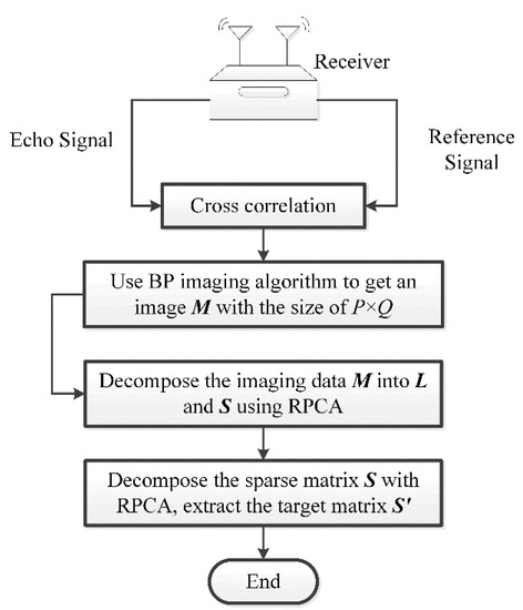
Figure 2.
Flow chart of the proposed method.
To quantitatively evaluate the proposed method, the signal-to-clutter ratio (SCR) is used as a criterion of image quality, which is defined as
where is the ith pixel in the image. Nt and Nc are the number of pixels in the target region Rt and pixels in the clutter region Rc, respectively. The larger the value of SCR, the better the result of the algorithm.
Figure 3 depicts the change in the value of λ versus the SCR in one experiment, where λ1 = 1/(λx)1/2 for the first RPCA and λ2 = 1/(λy)1/2 for the second RPCA. The red part means the higher SCR and the optimum value (λ1 = 1/(2005)1/2, λ2 = 1/(130)1/2) is given by the peak (the black point in the figure) of the SCR contour, where the highest SCR is approximately 34.40 dB. For comparison, the SCR curve varying with λx for the conventional RPCA is also given. We can find that the highest value is about 27.79 dB, which is lower than that of the proposed method. Therefore, our proposed method can improve the SCR through coarse-to-fine RPCA decomposition. Note that this result is obtained for the image with a size of 175 × 175, and it can be used for different circumstances as long as the image size is the same. Therefore, we use the optimized regularization parameters in all simulations and experiments. If the image size is changed, the parameters should be recomputed, or the subimage including the target with the same size is selected to suppress the clutter.
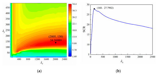
Figure 3.
Signal-to-clutter ratio (SCR) (dB) versus λ values for (a) the proposed method; (b) conventional robust principal component analysis (RPCA).
4. Results
In order to validate the proposed clutter removal method, both numerical simulation and real experiments are conducted. The synthesized data are generated by XFDTD software, and the laboratory experiment data are collected with chaos TWI radar developed by our research group. In the following experiments, the regularization parameters are set at λ1 = 1/(2005)1/2, λ2 = 1/(130)1/2 as optimized in Figure 3, and the image size is 175 × 175.
4.1. Numerical Simulation
The electromagnetic model with a human target is shown in Figure 5a. The length, width, and height of the room are 3.5 m. The human with a size of 0.2 m × 1.65 m (body radius × height, as shown in the top right corner) is located at (1.7, 2.0) m. The relative permittivity and the conductivity of the human are 50 and 1 mS/m, respectively [34]. The wall with a thickness of 0.2 m is assumed to be homogeneous, and its material is concrete (the relative permittivity is 4.5 and the conductivity is 0.03 mS/m [34]). The spatial grid of the model is 2.43 cm × 2.43 cm × 2.43 cm. The entire region uses the perfectly matched layer (PML) [35] as the truncated boundary. The PML is an artificial absorbing layer for wave equations to simulate problems with open boundaries. The receiving antenna with a height of 1.40 m is scanned 61 times along the x-axis (the blue points in Figure 5a represent some scanning positions) with a step size of 0.0243 m, and the number of sampling points per scan is 65537.
The emission direction of the electromagnetic wave is the y-axis, and the waveform is a chaotic pulse position modulation (CPPM) signal [36,37], which is composed of pulse sequences with equal amplitude and width. Its characteristic is that the inter-pulse intervals are modulated by a chaos map such as the logistic map, as shown in Figure 4a. The mathematical model of the CPPM signal is
where is the pulse waveform at time , is the initial time, and is the time interval between the nth and the (n−1)th pulse, which is produced by iterations of a nonlinear function . By choosing a with suitable parameters, will change in a chaotic way and has a random-like behavior. Here, we select the logistic map to modulate the pulse, which is defined as
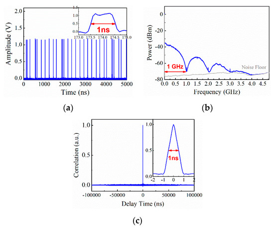
Figure 4.
Properties of the chaotic pulse position modulation (CPPM) signal. (a) Time series; (b) Power spectrum; (c) autocorrelation trace.
When k is set to 4, and is selected as 0.4, the output value of the logistic map varies between 0 and 1 and exhibits good random characteristics.
In our earlier work [10], a CPPM signal with 1 GHz bandwidth is generated from a field programmable gate array (FPGA), and the up-converted one is used as the transmitting signal in TWI radar [10] and life detection radar [38]. Simulation and experimental results have demonstrated that CPPM-based chaos TWI radar has good range resolution, unambiguous detection, and excellent jamming immunity to the noise and radio frequency interference. Besides that, the CPPM signal has a low crest factor, which can be used in the limited dynamics of real systems and it can eliminate the harmonics, since this kind of modulation smoothes the energy uniformly. Therefore, we select the CPPM signal as the transmitting signal to verify our proposed method.
Figure 4 shows the time series, power spectrum, and autocorrelation curve of the CPPM signal, which has been depicted in [10]. Obviously, the waveform has a delta-like autocorrelation, leading to high-range resolution.
The simulation results are presented in Figure 5. Figure 5b shows the cross-correlation image, which is generated by selecting the data corresponding to the imaging region from the matrix D. The red part of 0–0.5 m corresponds to the reflection of the front surface of the wall. Between 2 m and 3 m at the down range, the body’s reflection shows a hyperbolic curve, in which the energy is not focused. Figure 5c indicates the BP imaging result. The reflection energy of the human is well focused. The first-stage RPCA result (called BP-RCPA2-1) is shown in Figure 5d. We can see that the wall reflection disappears, but there is still some clutter in the background, so the subsequent decomposition can be performed. The result of the proposed method is shown in Figure 5e. We can see that the wall reflection disappears, and the target is very clearly, nearly without ghosts. Note that the human target is distinct, but its position at the down range is slightly farther away than 2.0 m, because the distance is calculated in free space and the thickness of the wall is ignored. Besides that, the clutter in the simulation is mainly the wall clutter, since there are no other objects in the background and the antenna is assumed as the observation point, not the real antenna.
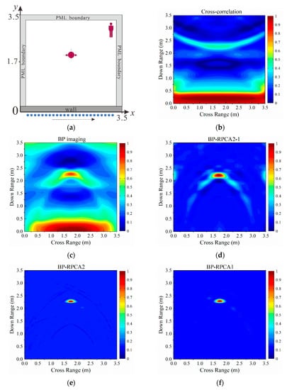
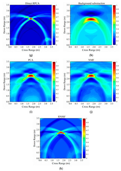
Figure 5.
Simulation results of a single target. (a) Simulation model for through-wall detection; (b) Cross-correlation result; (c) Back-projection (BP) imaging; (d) The first stage of BP-RPCA2; (e) BP-RPCA2; (f) BP-RPCA1; (g) Direct RPCA; (h) Background subtraction; (i) Principal component analysis (PCA); (j) Nonnegative matrix factorization (NMF); (k) Robust nonnegative matrix factorization (RNMF).
To demonstrate the superiority of the proposed method, one-stage RPCA with an optimized regularization parameter (λ = 1/(260)1/2) (referred to as BP-RPCA1), the direct RPCA decomposition method [24,25] (direct RPCA) with an optimized regularization parameter (λ = 1/(2200)1/2), the background subtraction method, PCA, nonnegative matrix factorization (NMF) [39], and RNMF [28] are applied to cross-correlation data for comparison. Note that except for BP-RPCA1, other methods are used before imaging, as in the conventional clutter suppression method.
The results are shown in Figure 5f–k. It can be found that the performance of BP-RCPA1 is similar to that of the proposed method when the clutter is not high. The direct RPCA decomposition eliminates the low-rank component of the cross-correlation data. The clutter is suppressed to some extent, but its performance is less effective compared with our proposed method. For the background subtraction method, the reflection of the wall disappears. and we can get the position of the human body. However, there are still some ghosts around the target. PCA and NMF present similar visual results, containing some ghosts that remain. RNMF has a similar result to direct RPCA.
Table 1 lists the SCR values of the above methods. The best SCR values are obtained by our proposed method followed by BP-RPCA1 and RNMF, which is consistent with the results in Figure 5. The corresponding running times are also given. All the methods are tested on an Intel Core i74790 at 3.6-GHz, 16-GB RAM, on a Windows 10 64-bit environment. Obviously, the direct RPCA is time-consuming, since it works on the correlation matrix, whose size is 131073 × 61, while the proposed method works on the focused 175 × 175 image, leading to a greatly shorter running time. For PCA and the NMF method, the computation time is also short, but the performance is not very good. RNMF has less running time than direct RPCA, but it is higher than our proposed method. Therefore, considering both image quality and running time, the proposed method is the best choice.

Table 1.
Quantitative analysis of different clutter removal methods in simulation.
To further demonstrate the originality of the proposed imaging-then-decomposition clutter suppression method, and explain the BP algorithm effect in this method, the sparsity of the target matrix is analyzed quantitatively. According to [20,29], the constant in Equation (3) can be used as the measure of the matrix’s sparsity. The smaller ρs corresponds to a more sparse matrix. Since the target responses are contained in the sparse matrix, the more focused they are, the more sparse the sparse matrix. For our proposed method and direct RPCA method, the ρs value of the normalized sparse component is 0.091 and 0.308, respectively. Here, zero entries of the sparse matrix are the elements that less than a threshold, i.e., 0.01. From the ρs values, it can be concluded that the BP algorithm can improve the sparsity, which is why a better decomposition is obtained.
Note that in the above simulation, we just consider the front wall in the scene. Indeed, even if the back wall exists, our proposed method can still perform well. Figure 6 presents a simulation result. The scene is the same as in Figure 5a; only a back wall with a thickness of 0.2 m is added. We can find that the reflection from the front wall and the back wall are both removed (for BP imaging, the reflection of the back wall is different of that of the front wall, since we did not consider the wall effect, and the delay time is not calibrated).
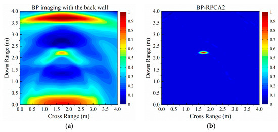
Figure 6.
Simulation results of a single target with the back wall. (a) BP imaging; (b) BP-RPCA2.
A multi-target experiment is also presented in Figure 7. In this case, two persons are located at (1.1,1.1) m and (2.2,2.2) m, respectively. It can be seen that after using our proposed method, the clutter is less remained and two targets are more clearly identified compared with the results of other methods. Note that BP-RPCA1 with optimized (λ = 1/(160)1/2) has lower contrast than BP-RPCA2. The images of direct RPCA (λ = 1/(2100)1/2) and RNMF both contain hyperbola signatures. The SCR values are also shown in Table 1. Similar to the results of a single-target experiment, BP-RPCA2 presents the best SCR value with less running time.
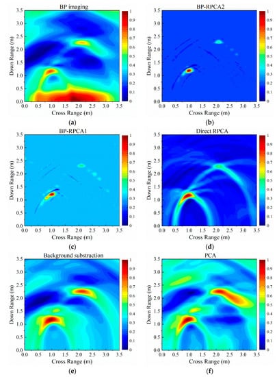
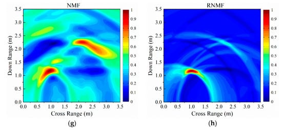
Figure 7.
Simulation results of multiple targets. (a) BP imaging; (b) BP-RPCA2; (c) BP-RPCA1; (d) Direct RPCA; (e) Background subtraction; (f) PCA; (g) NMF; and (h) RNMF.
4.2. Laboratory Experiments
The experimental setup of chaos TWI radar is shown in Figure 8a, which is developed by our research group, and its details can be found in [10]. The chaotic signal is also a CPPM signal used in the simulation, and it is up-converted to 2.4 GHz as the radar transmitting signal. The average power of the emitted radiation is 8.3 dBm, which is measured by an average power sensor, as mentioned in [10]. A cinder block wall with a thickness of 0.2 m is constructed, and it has about 30 dB transmission loss at 2.4 GHz [10]. After wall attenuation, the power captured by the receiving antenna is only –53.2 dBm, so the amplifier is used. The antennas with 0.2 m separation are broadband horn antennas with a bandwidth of 1 to 18 GHz. They are fixed at the scanner and moved horizontally along the wall with a step size of 0.05 m. The number of scanning positions is 51, and the number of sampling points per scan is 125,000. The image area is 3.5 m × 3.5 m, and a person behind the wall is located at (1.3,1.5) m, as shown in Figure 8b,c.
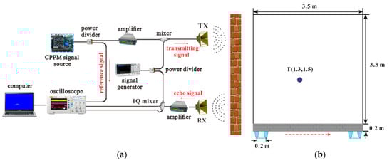
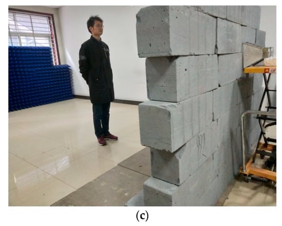
Figure 8.
Experiment setup. (a) Chaos through-wall imaging (TWI) radar system; (b) Scene layout; (c) Scenario of a standing man in the laboratory.
Figure 9a shows the range matrix after cross-correlation computation, where line signatures are obvious, and the target barely can be found. After BP imaging, the energy of the target response is enhanced, but strong clutter is dominant and the target is still submerged, as shown in Figure 9b. The BP-RPCA2 result is depicted in Figure 9c, where strong wall reflection and most of the clutter are removed, and the target is distinct, whose position is close to the real value. Note that the wall in the experiment is indeed heterogeneous, which will affect the propagation time of the electromagnetic wave through the wall, and thus affect the range of the target, so the range is calibrated in the experiment by placing a metallic plate behind the wall to find the delay due to the system and the wall effect.
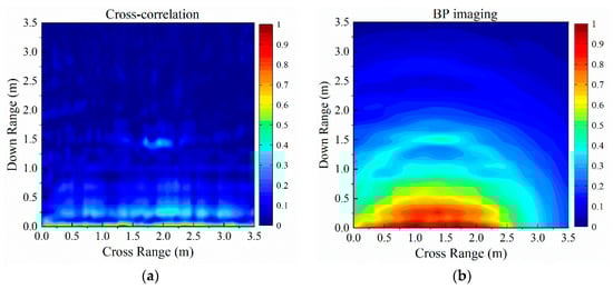
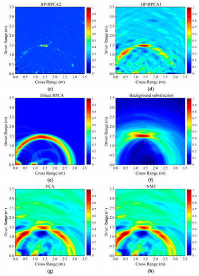
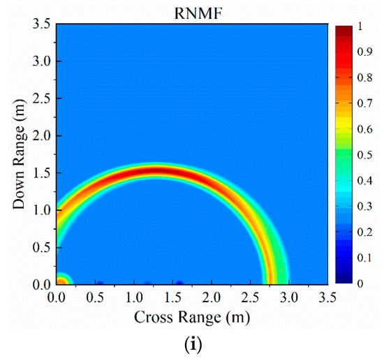
Figure 9.
Experiment results of single target. (a) Cross-correlation result; (b) BP imaging; (c) BP-RPCA2; (d) BP-RPCA1; (e) Direct RPCA; (f) Background subtraction; (g) PCA; (h) NMF; and (i) RNMF.
For comparison, BP-RPCA1 (λ = 1/(1740)1/2), direct RPCA (λ = 1/(225)1/2), background subtraction, PCA, NMF, and RNMF are also implemented. The results are shown in Figure 9d–i. It can be found that BP-RPCA1 presents a worse result than BP-RPCA2, although the regularization parameter λ is optimized. For the direct RPCA method, a distinct hyperbola is presented around the target position, but strong wall reflection also remains. RNMF has a comparable result to direct RPCA, but with better wall reflection suppression. The SCR values of different methods are listed in Table 2. Again, our proposed method has the highest SCR value among all the other methods, which is in accordance with the results in Figure 9. Besides that, the proposed method is time-saving compared with direct RPCA and RNMF methods.
Table 2.
Quantitative analysis of different clutter removal methods in experiment.
Figure 10 presents the multi-target experimental results. In the BP imaging result, wall reflections are dominant and the targets are not obvious, especially for the person far from the antenna. After using our proposed method, most of the strong wall clutter is removed and both of the two targets are distinct, although the farther one is weak to some extent. For the BP-RPCA1 (λ = 1/(400)1/2) method, the wall reflection is not removed completely, and the targets are less clear than BP-RPCA2. From all the simulation and experimental results, we can find that two-stage RPCA has better performance than one-stage RPCA, especially in complex and heavy clutter cases. Direct RPCA (λ = 1/(240)1/2) and RNMF present similar results, which contain hyperbola curves around the target positions. The corresponding SCR values and running times are also provided in Table 2. Similarly, our proposed method has the best SCR value followed by BP-RPCA1 and RNMF, and has less running time than direct RPCA and RNMF. Note that our proposed method BP-RPCA2 is about 14 times faster than direct RPCA. Thus, in addition to its higher visual performance, it is suitable to work in real time.
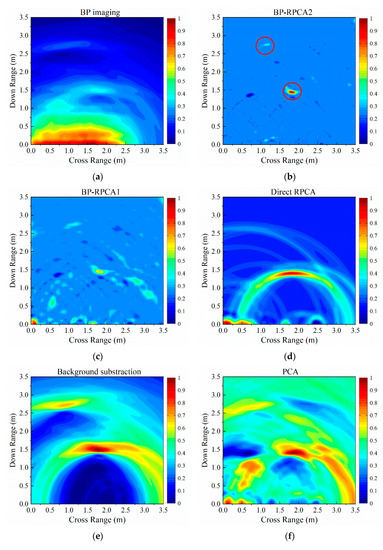
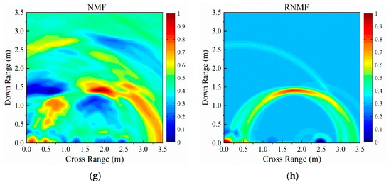
Figure 10.
Experiment results of multiple targets. (a) BP imaging; (b) BP-RPCA2; (c) BP-RPCA1; (d) Direct RPCA; (e) Background subtraction; (f) PCA; (g) NMF; (h) RNMF.
5. Conclusions
In this paper, an imaging-then-decomposition clutter suppression method based on two-stage RPCA is proposed for chaos TWI radar. Instead of decomposing the raw data, the presented method firstly strengthens the energy of cross-correlation data by the BP imaging method and then performs optimized RPCA twice to suppress the clutter and indicate the target.
Simulation and experimental results of single/multiple targets demonstrate that the proposed method can effectively suppress the clutter, reveal the location of human targets, and thus enhance the SCR ratio, which is beneficial for further identification. It possesses superiority in comparison to background subtraction, PCA, NMF, and RNMF methods. Compared with the conventional direct RPCA decomposition method, it has a higher SCR value and greatly faster computation time. Compared with one-stage optimized RPCA, it is more effective in real applications and heavy clutter environments. We also try to apply RPCA three times after BP imaging (called BP-RPCA3), but we find that the SCR value just increases a little while the running time is about 1.4 times. It is also time-consuming to optimize the regularization parameters for BP-RPCA3. Besides that, there is a risk of losing the weak target, since the weak target may be considered as the background clutter and removed in the third decomposition. Additionally, the running time analysis in this paper is performed on a PC. In real applications, the proposed algorithm can be implemented on an embedded system, such as FPGA, since an implementation of RPCA on FPGA has been proposed [40], and thus the time will be greatly reduced in an order of one or two by conservative estimation, which is beneficial to real-time applications.
Note that identical to other general clutter removal methods (e.g., PCA, SVD, ICA), the proposed method can be used in most of the TWI scenarios with other types of wall materials (e.g., brick, concrete, wood, asbestos; metallic is excluded). Moreover, it can be applied to other radar systems if ignoring cross-correlation processing. Future work will focus on improving the method to tackle multiple targets with low reflections.
Author Contributions
Conceptualization, L.L.; experimental work, Q.C. and Y.H.; writing—original draft preparation, Y.H.; writing—review and editing, L.L. and H.X.; supervision, L.L. and H.X.; funding acquisition, L.L., H.X., J.L. and B.W. All authors have read and agreed to the published version of the manuscript.
Funding
This research was funded by the National Natural Science Foundation of China, grant number 41704147, 41604127, 61601319, the Natural Science Foundation of Shanxi Province, grant number 201801D221185, 201801D121140, and the Key Research and Development (R&D) Project of Shanxi Province, grant number 201703D321036, 201803D31037.
Conflicts of Interest
The authors declare no conflict of interest.
References
- Baranoski, E.J. Through-wall imaging: Historical perspective and future directions. J. Franklin Inst. 2008, 345, 556–569. [Google Scholar] [CrossRef]
- Narayanan, R.M. Through-wall radar imaging using UWB noise waveforms. J. Franklin Inst. 2008, 345, 659–678. [Google Scholar] [CrossRef]
- Lai, C.P.; Narayanan, R.M. Ultrawideband random noise radar design for through-wall surveillance. IEEE Trans. Aerosp. Electron. Syst. 2010, 46, 1716–1730. [Google Scholar] [CrossRef]
- Susek, W.; Stec, B. Through-the-wall detection of human activities using a noise radar with microwave quadrature correlator. IEEE Trans. Aerosp. Electron. Syst. 2015, 51, 759–764. [Google Scholar] [CrossRef]
- Liu, Z.; Zhu, X.; Hu, W.; Jiang, F. Principles of chaotic signal radar. Int. J. Bifurc. Chaos 2007, 17, 1735–1739. [Google Scholar] [CrossRef]
- Pappu, C.S.; Flores, B.C.; Debroux, P.S.; Verdin, B.; Boehm, J. Synchronisation of bistatic radar using chaotic AM and chaos-based FM waveforms. IET Radar Sonar Navig. 2017, 11, 90–97. [Google Scholar] [CrossRef]
- Venkatasubramanian, V.; Leung, H.; Liu, X. Chaos UWB radar for through-the-wall imaging. IEEE Trans. Image Process. 2009, 18, 1255–1265. [Google Scholar] [CrossRef]
- Quan, Y.; Li, Y.; Hu, W.; Zhai, Y.; Xing, M. FM sequence optimisation of chaotic-based random stepped frequency signal in through-the-wall radar. IET Signal Process. 2017, 11, 830–837. [Google Scholar] [CrossRef]
- Liu, L.; Ma, R.; Li, J.; Zhang, J.; Wang, B. Anti-jamming property of Colpitts-based direct chaotic through-wall imaging radar. J. Electromagn. Wave 2016, 30, 2268–2279. [Google Scholar] [CrossRef]
- Xu, H.; Wang, B.; Zhang, J.; Liu, L.; Li, Y.; Wang, Y.; Wang, A. Chaos through-wall imaging radar. Sens. Imaging 2017, 18, 6. [Google Scholar] [CrossRef]
- Solimene, R.; Cuccaro, A. Front wall clutter rejection methods in TWI. IEEE Geosci. Remote Sens. Lett. 2013, 11, 1158–1162. [Google Scholar] [CrossRef]
- Verma, P.K.; Gaikwad, A.N.; Singh, D.; Nigam, M.J. Analysis of clutter reduction techniques for through wall imaging in UWB range. Prog. Electromagn. Res. 2009, 17, 29–48. [Google Scholar] [CrossRef]
- Gaikwad, A.N.; Singh, D.; Nigam, M.J. Application of clutter reduction techniques for detection of metallic and low dielectric target behind the brick wall by stepped frequency continuous wave radar in ultra-wideband range. IET Radar Sonar Navig. 2011, 5, 416–425. [Google Scholar] [CrossRef]
- Singh, A.P.; Jain, P.K. Acompartive study of SVD and ICA for target detectionin through-the-wall radar images. In Proceedings of the 2016 11th International Conference on Industrial and Information Systems (ICIIS), Roorkee, India, 3–4 December 2016; pp. 608–613. [Google Scholar]
- Guo, S.; Yang, X.; Cui, G.; Song, Y.; Kong, L. Multipath ghost suppression for through-the-wall imaging radar via array rotating. IEEE Geosci. Remote Sens. Lett. 2018, 15, 868–872. [Google Scholar] [CrossRef]
- Bivalkar, M.; Singh, D.; Kobayashi, H. Entropy-based low-rank approximation for contrast dielectric target detection with through wall imaging system. Electronics 2019, 8, 634. [Google Scholar] [CrossRef]
- Nkwari, P.K.M.; Sinha, S.; Ferreira, H.C. Through-the-wall radar imaging: A review. IETE Tech. Rev. 2018, 35, 631–639. [Google Scholar] [CrossRef]
- Yoon, Y.S.; Amin, M.G. Spatial filtering for wall-clutter mitigation in through-the-wall radar imaging. IEEE Trans. Geosci. Remote Sens. 2009, 47, 3192–3208. [Google Scholar] [CrossRef]
- Tivive, F.H.C.; Bouzerdoum, A.; Amin, M.G. A subspace projection approach for wall clutter mitigation in through-the-wall radar imaging. IEEE Trans. Geosci. Remote Sens. 2015, 53, 2108–2122. [Google Scholar] [CrossRef]
- Candes, E.J.; Li, X.; Ma, Y.; Wright, J. Robust Principal Component Analysis? J. ACM 2011, 58, 1–37. [Google Scholar] [CrossRef]
- Zhang, Y.; Xia, T. In-wall clutter suppression based on low-rank and sparse representation for through-the-wall radar. IEEE Geosci. Remote Sens. Lett. 2016, 13, 671–675. [Google Scholar] [CrossRef]
- Tang, V.H.; Bouzerdoum, A.; Phung, S.L.; Tivive, F.H.C. Indoor scene reconstruction for through-the-wall radar imaging using low-rank and sparsity constraints. In Proceedings of the 2016 IEEE Radar Conference (RadarConf), Philadelphia, PA, USA, 2–6 May 2016; pp. 1–4. [Google Scholar]
- Tang, V.H.; Bouzerdoum, A.; Phung, S.L. Multipolarization through-wall radar imaging using low-rank and jointly-sparse representations. IEEE Trans. Image Process. 2018, 27, 1763–1776. [Google Scholar] [CrossRef] [PubMed]
- Qiu, L.; Jin, T.; He, Y.; Lu, B.Y.; Zhou, Z.M. Sparse and low-rank matrix decomposition based micro-motion target indication in through-the-wall radar. Electron. Lett. 2017, 53, 191–192. [Google Scholar] [CrossRef]
- Kalika, D.; Knox, M.T.; Collins, L.M.; Torrione, P.A.; Morton, K.D., Jr. Leveraging robust principal component analysis to detect buried explosive threats in handheld ground-penetrating radar data. In Proceedings of the SPIE Detection and Sensing of Mines, Explosive Objects, and Obscured Targets XX, Baltimore, MD, USA, 21 May 2015; Volume 9454, p. 94541D. [Google Scholar]
- Zhang, Y.; Xia, T. Extracting sparse crack features from correlated background in ground penetrating radar concrete imaging using robust principal component analysis technique. In Proceedings of the SPIE Nondestructive Characterization and Monitoring of Advanced Materials, Aerospace, and Civil Infrastructure, Las Vegas, NV, USA, 8 April 2016; Volume 9804, p. 980402. [Google Scholar]
- Song, X.; Xiang, D.; Zhou, K.; Su, Y. Improving RPCA-based clutter suppression in GPR detection of antipersonnel mines. IEEE Geosci. Remote Sens. Lett. 2017, 14, 1338–1342. [Google Scholar] [CrossRef]
- Kumlu, D.; Erer, I. Improved Clutter Removal in GPR by Robust Nonnegative Matrix Factorization. IEEE Geosci. Remote Sens. Lett. 2019, in press. [Google Scholar]
- Zhou, Z.; Li, X.; Wright, J.; Candes, E.; Ma, Y. Stable principal component pursuit. In Proceedings of the 2010 IEEE International Symposium on Information Theory, Austin, TX, USA, 13–18 June 2010; pp. 1518–1522. [Google Scholar]
- Lin, Z.; Liu, R.; Su, Z. Linearized alternating direction method with adaptive penalty for low-rank representation. Adv. Neural Inf. Process. Syst. 2011, 2011, 612–620. [Google Scholar]
- Chen, X.; Leung, H.; Tian, M. Multitarget detection and tracking for through-the-wall radars. IEEE Trans. Aerosp. Electron. Syst. 2014, 50, 1403–1415. [Google Scholar] [CrossRef]
- Ahmad, F.; Amin, M.G.; Kassam, S.A. Synthetic aperture beamformer for imaging through a dielectric wall. IEEE Trans. Aerosp. Electron. Syst. 2005, 41, 271–283. [Google Scholar] [CrossRef]
- Cui, G.; Kong, L.; Yang, J. A back-projection algorithm to stepped-frequency synthetic aperture through-the-wall radar imaging. In Proceedings of the 1st Asian and Pacific Conference on Synthetic Aperture Radar, Huangshan, China, 5–9 November 2007; pp. 123–126. [Google Scholar]
- Wang, H.; Narayanan, R.M.; Zhou, Z.O. Through-wall imaging of moving targets using UWB random noise radar. IEEE Antennas Wirel. Propag. Lett. 2009, 8, 802–805. [Google Scholar] [CrossRef]
- Johnson, S.G. Notes on perfectly matched layers (PMLs). Lect. Notes Mass. Inst. Technol. Mass. 2008, 29, 1–16. [Google Scholar]
- Sushchik, M.; Rulkov, N.; Larson, L.; Tsimring, L.; Abarbanel, H.; Yao, K.; Volkovskii, A. Chaotic pulse position modulation: A robust method of communicating with chaos. IEEE Commun. Lett. 2000, 4, 128–130. [Google Scholar] [CrossRef]
- Rulkov, N.F.; Sushchik, M.M.; Tsimring, L.S.; Volkovskii, A.R. Digital communication using chaotic-pulse-position modulation. IEEE Trans. Circuits Syst. I Fundam. Theor. Appl. 2001, 48, 1436–1444. [Google Scholar] [CrossRef]
- Xu, H.; Li, Y.; Zhang, J.; Han, H.; Zhang, B.; Wang, L.; Wang, Y.; Wang, A. Ultra-wideband chaos life-detection radar with sinusoidal wave modulation. Int. J. Bifurc. Chaos 2017, 27, 1730046. [Google Scholar] [CrossRef]
- Kumlu, D.; Erer, I. Clutter removal in GPR images using non-negative matrix factorization. J. Electromagn. Wave. 2018, 32, 2055–2066. [Google Scholar] [CrossRef]
- Karunaratne, M.; Samarawickrama, J. Low rank matrix estimation using robust principal component analysis on FPGA. In Proceedings of the 7th International Conference on Information and Automation for Sustainability, Colombo, Sri Lanka, 22–24 December 2014; pp. 1–6. [Google Scholar]
© 2019 by the authors. Licensee MDPI, Basel, Switzerland. This article is an open access article distributed under the terms and conditions of the Creative Commons Attribution (CC BY) license (http://creativecommons.org/licenses/by/4.0/).