Large-Scale Outdoor SLAM Based on 2D Lidar

Abstract

For autonomous driving, it is important to navigate in an unknown environment. In this paper, we propose a fully automated 2D simultaneous localization and mapping (SLAM) system based on lidar working in large-scale outdoor environments. To improve the accuracy and robustness of the scan matching module, an improved Correlative Scan Matching (CSM) algorithm is proposed. For efficient place recognition, we design an AdaBoost based loop closure detection algorithm which can efficiently reject false loop closures. For the SLAM back-end, we propose a light-weight graph optimization algorithm based on incremental smoothing and mapping (iSAM). The performance of our system is verified on various large-scale datasets including our real-world datasets and the KITTI odometry benchmark. Further comparisons to the state-of-the-art approaches indicate that our system is competitive with established techniques.

1. Introduction

Simultaneous localization and mapping (SLAM) is one of the key problems for an autonomous mobile robot and has been actively researched for over two decades [1]. As a fundamental module of mobile robot, SLAM has wide application domains ranging from exploration to autonomous driving. While other sensor modalities such as IMU, camera, GPS or RGBD sensors are commonly used, SLAM based on lidar sensor has been very popular, in part because lidar sensor has the advantages of high precision and strong resistance to interference, and is robust to illumination variations. In particular, in this work we focus on large-scale outdoor SLAM based on 2D lidar sensor. 2D lidar sensor enjoys the merits of both high-accuracy range measurement and low-cost compared to the expensive 3D lidar scanners, making it a more suitable choice for cost-sensitive application scenarios.

Typically, a lidar SLAM system consists of a lidar odometry front-end and a back-end that performs the pose graph optimization to obtain a globally optimized map and the full trajectory of the robot. Besides, loop closure detection plays an important role that provides constraints between poses that were captured at the same place but at different times. For the front-end, Iterative Closest Point (ICP) [2], Normalized Distribution Transform (NDT) [3] and Correlative Scan Matcher (CSM) [4] are typical algorithms that were commonly used for 2D lidar scan matching. In particular, ICP and NDT are efficient local scan matching algorithms that depend on an accurate initial guess, but may get stuck in a local optimum if the initial guess is far from the ground-truth. On the contrary, CSM is a global scan matching algorithm that could find the global optimum at a fixed resolution in a probabilistic framework. Various approaches [5,6] have been proposed to improve the performance of CSM for 2D lidar scan matching. Previous works have obtained satisfactory results in relatively small indoor environment, whilst the application in large-scale outdoor environment is still a challenging task.

The primary challenges in designing a 2D lidar SLAM system for large-scale outdoor environment lie in three aspects: Firstly, the front-end should be designed computationally-efficient and robust to initialization error, generating a good prior for loop closure detection and global optimization, especially in low-texture and dynamic environment. Secondly, an efficient loop closure detection algorithm is needed to reduce accumulation drift when loops are detected. This is of particular importance in large-scale settings. However, most existing loop closure detection algorithms are designed for visual SLAM systems [7,8,9,10], and little attention has been given to 2D lidar SLAM systems [11,12,13]. Finally, an accurate and robust optimization back-end is needed to reject false loop closures.

To tackle the above challenges, this paper makes the following three contributions:

(1)

Firstly, a modified CSM algorithm is proposed to improve the accuracy and robustness of the front-end scan matching algorithm, especially in low-texture and dynamic environment.

(2)

Secondly, we propose an AdaBoost based loop closure detection algorithm and a false loop closure rejection algorithm which work efficiently to perform place recognition.

(3)

Thirdly, we propose a light-weight back-end optimization algorithm that works in real-time. The optimization results are also utilized to eliminate false loop closures.

The remainder of this paper is organized as follows. In Section 2, some related works are introduced. The details of the implementation of our approach are presented in Section 3. Section 4 provides the experimental results and comparisons with state-of-the-art approaches on both publicly available datasets and our own collected datasets. Finally, the conclusions and future works are summarized in Section 5.

2. Related Works

2.1. Scan Matching Approaches

The aim of scan matching [14] is to estimate the rigid-body transformation between two laser scans. The Iterative Closest Point (ICP) [2] and Iterative Closest Line [15] are the most popular scan matching algorithms which estimate the relative transform by finding the nearest points between the two laser scans. Zhang et al. [16] proposed a low-drift and real-time lidar odometry and mapping (LOAM) algorithm, which selects feature points based on the roughness of the point’s local region. The feature points are then matched using either point-to-line or point-to-plane distances. There have been other scan matching approaches, including NDT [3], hough transform-based approaches [17] and histogram-based approaches [18,19]. All these approaches rely on some model assumptions, and may get stuck in a local optimum, especially in large-scale, low-texture and dynamic environments.

Olson et al. [4] proposed the Correlative Scan Matcher (CSM) to search for the best rigid transformation in a probabilistic framework. Compared with other scan matching approaches, CSM is robust to large initialization errors while running in real-time by utilizing the multi-resolution lookup-table rasterization technique. Chong et al. [5] proposed the Extended Correlative Scan Matcher (ECSM) which improves the scan matching accuracy with surface normal information.

2.2. Loop Closure Detection

There have been works based on Monte Carlo localization [20] and Rao-Blackwellized filtering [21] to tackle the 2D lidar loop closure detection problem. Recent works on loop closure detection can be roughly classified into three categories: feature based approaches, optimization based approaches and learning based approaches [13].

Bosse et al. [22] proposed to use orientation histogram and projection histogram for loop closure detection. Himstedt et al. [23] augmented the original Fast Laser Interest Point Transform (FLIRT) [24] descriptor with the orientation and distances of landmarks to accelerate place recognition. The approach of cartographer [12] firstly built submaps and then aligned scans to submaps to generate closed loops by a branch-and-bound approach. Li et al. [13] utilized deep learning to perform loop closure detection in indoor environment. The most similar work to our approach is the method proposed in [11], which treat the loop closure detection problem as a classification problem, and use AdaBoost to detect loop closures.

2.3. Pose Graph Optimization

There exists several graph-based back-end optimization algorithms, including iSAM [25], iSAM2 [26], g2o [27], etc. Some recent researches focused on utilizing these algorithms to reject false loop closures, such as the Max-Mixture Model [28], Switchable Constraints [29], and Realizing, Reversing, Recovering (RRR) [30]. The analysis of [31] showed that none of these methods work perfectly.

3. Methodology

As shown in Figure 1, our full system mainly contains three parts: The front-end (Section 3.1), the loop closure detection part (Section 3.2) and the back-end (Section 3.3). The front-end is in charge of key frame selection, data preprocessing, point cloud feature extraction and scan matching. The loop closure detection part is responsible for the detection and validation of the loop closures. The back-end optimizes vehicle poses and global map based on the loop closure detection results and the scan matching results obtained from the front-end. Unlike traditional descriptions, we separate the loop closure part from the front-end to emphasize its importance, especially in mapping large-scale outdoor environment.

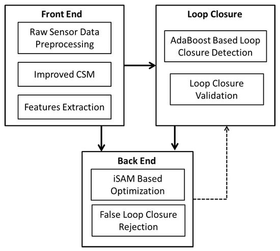
Figure 1. The overview of our 2D-SLAM system.

3.1. Front-End Based on Improved CSM

3.1.1. Probabilistic Formulation and CSM Overview

Given two lidar scans, CSM is applied to calculate the optimal rigid body transform between the two lidar poses. The scan matching problem can be described in a probabilistic framework. Let the vehicle move from $x_{i-1}$ to $x_i$, with motion u obtained from the IMU and the wheel encoder. The goal of scan matching is to find the maximum posterior probability $p\left(x_i\right|x_{i-1},u,m,z)$, where m is the environment model and z is the current observation. According to Bayes rule, we have

$$p\left(x_i\right|x_{i-1},u,m,z)\propto p\left(z\right|x_i,m)p\left(x_i\right|x_{i-1},u).$$

(1)

Supposing every lidar observation $z_j$ is independent, the observation model can be written as

$$p\left(z\right|x_i,m)=\prod _{j}p\left(z_j\right|x_i,m).$$

(2)

In the context of scan matching, we set the target scan as $\mathcal{P}$, and the source scan as $\mathcal{Q}$. Let $\mathcal{T}$ be the rigid body transform that transforms points in $\mathcal{Q}$ into $\mathcal{P}$’s coordinate. The observation model can be written as

$$p\left(z\right|x_i,m)=p\left(\mathcal{Q}\right|\mathcal{T},\mathcal{P})=p\left(\mathcal{T}\left(\mathcal{Q}\right)\right|\mathcal{P}).$$

(3)

Based on Equations (2) and (3), the problem of finding the optimal transformation ${\mathcal{T}}^{*}$ is thus equivalent to search for the maximum log likelihood of the observation model

$$\begin{array}{cc}\hfill {\mathcal{T}}^{*}& =\arg \underset{\mathcal{T}}{\max }\log p\left(\mathcal{T}\left(\mathcal{Q}\right)|\mathcal{P}\right)\hfill \\ & =\arg \underset{\mathcal{T}}{\max }\log \prod _{i}p\left(\mathcal{T}\left({\mathcal{Q}}_i\right)|{\mathcal{P}}_{raster}\right)\hfill \\ & =\arg \underset{\mathcal{T}}{\max }\sum _i\log p\left(\mathcal{T}\left({\mathcal{Q}}_i\right)|{\mathcal{P}}_{raster}\right),\hfill \end{array}$$

(4)

where ${\mathcal{P}}_{raster}$ stands for the grid map rasterized from the target scan $\mathcal{P}$ and ${\mathcal{Q}}_i(i\in N)$ is a single point of scan $\mathcal{Q}$. $\mathcal{T}$ corresponds to a 3*3 homogeneous matrix, defined as

$$\mathcal{T}=\left[\begin{array}{ccc}cos{\xi }_{\theta }& -sin{\xi }_{\theta }& {\xi }_x\\ sin{\xi }_{\theta }& cos{\xi }_{\theta }& {\xi }_y\\ 0& 0& 1\end{array}\right].$$

(5)

3.1.2. The Improved Correlative Scan Matcher

The multi-resolution CSM proposed in [4,5,6] is described in Algorithm 1. This approach could obtain satisfactory results in most structured environment; however, it will encounter difficulties in handling large-scale, low-texture, and dynamic environment, especially for corridors and tunnels. Based on this algorithm, we make the following improvements:

Algorithm 1 The multi-resolution CSM algorithm

Require: Target scan $\mathcal{P}$, Source scan $\mathcal{Q}$, Initial guess ${\mathcal{T}}_0$  1: Rasterization of lookup table: $L_{high}$, $L_{low}$  2: Initialization of scan matching score and transformation: $S_L^{best}\leftarrow 0$, $S_H^{best}\leftarrow 0$, ${\mathcal{T}}_L^{*}\leftarrow {\mathcal{T}}_0$  3: for$i=1$ to N do  4:  $S_L^i\leftarrow {\sum }_{k=1}^m{L}_{low}\left({\mathcal{T}}_i{q}_k\right)$ where $q_k\in \mathcal{Q}$ and ${\mathcal{T}}_i=△{\mathcal{T}}_i{\mathcal{T}}_L^{*}$  5:  if $S_L^i>S_L^{best}$ then  6:   $S_L^{best}\leftarrow S_L^i,{\mathcal{T}}_L^{*}\leftarrow {\mathcal{T}}_i$  7:  end if  8: end for  9: for$j=1$ to M do 10:  $S_H^j\leftarrow {\sum }_{k=1}^m{L}_{high}\left({\mathcal{T}}_j{q}_k\right)$ where $q_k\in \mathcal{Q}$ and ${\mathcal{T}}_j=△{\mathcal{T}}_j{\mathcal{T}}_L^{*}$ 11:  if $S_H^j>S_H^{best}$ then 12:   $S_H^{best}\leftarrow S_H^j,{\mathcal{T}}_H^{*}\leftarrow {\mathcal{T}}_j$ 13:  end if 14: end for 15: ${\mathcal{T}}^{*}\leftarrow {\mathcal{T}}_H^{*}$ 16: return${\mathcal{T}}^{*}$

(1) Firstly, we improved the rasterization of the lookup table. Instead of rasterizing the single target scan, we utilize historical multi-frame to generate a more robust and more comprehensive rasterized cost table. The multi-frame rasterization algorithm is summarized in Algorithm 2, and the comparison with traditional rasterization approach is shown in Figure 2. To increase the accuracy of the raster table, a weighted sum of historical raster tables can be used, as shown in line 7 of Algorithm 2. A scan that is far away from the current scan will be set a smaller weight.

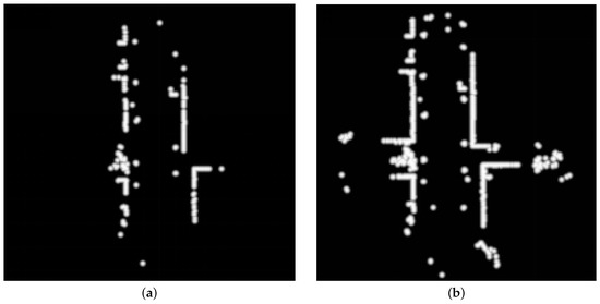
Figure 2. The comparative results of different rasterization methods. (a) Rasterized cost table from single scan. (b) Rasterized cost table from multiple scans.

Algorithm 2 The multi-frame rasterization algorithm

1: Initialization of the look up table  2: for$i=t-k$ to $t-1$ do  3:  Transform historical scan ${\chi }_i$ to coordinate $t-1$:  4:  ${\chi }_i^{{}^{\prime }}\leftarrow {\mathcal{T}}_{i,t-1}{\chi }_i$  5:  for $j=1$ to $n_i$ do  6:   Rasterization of ${\chi }_i^{{}^{\prime }}$:  7:   $p_j\leftarrow {\omega }_i{L}^{\left(j\right)}\left({\chi }_i^{{}^{\prime }}\right)$  8:   if $p_j>p_j^{*}$ then  9:    $p_j^{*}\leftarrow p_j$ 10:   end if 11:   $L^{\left(j\right)}\left({\chi }_{t-1}\right)\leftarrow p_j^{*}$ 12:  end for 13: end for 14: return$L\left({\chi }_{t-1}\right)$

(2) Secondly, the covariance of the transformation $\mathcal{T}$ is utilized to recognize scenes that have high matching uncertainty, such as corridors or tunnels. Similar to [4], we calculate the mean and the covariance for $\mathcal{T}$ as follows: Suppose ${\mathcal{T}}_i$ is a particle corresponding to a single transform along with its weight $S_i$, $\{{\mathcal{T}}_i,S_i\}$ is the posterior distribution of $\mathcal{T}$. Let ∑ be the covariance of transformation $\mathcal{T}$, we have

$$\left\{\begin{array}{c}\begin{array}{cc}\hfill K& =\sum _i{\mathcal{T}}_i{\mathcal{T}}_i^T{S}_i\hfill \\ \hfill u& =\sum _i{\mathcal{T}}_i{S}_i\hfill \\ \hfill s& =\sum _i{S}_i\hfill \\ \hfill \sum & =\frac{1}{s}K-\frac{1}{s^2}u{u}^T\hfill \end{array}\hfill \end{array}.\right.$$

(6)

Let ${\sum }_x,{\sum }_y,{\sum }_z$ be the diagonal values of $\sum$, we define ${\sum }_l$ and ${\sum }_s$ as

$$\left\{\begin{array}{c}\begin{array}{cc}\hfill {\sum }_l& =\max \{{\sum }_x,{\sum }_y\}\hfill \\ \hfill {\sum }_s& =\min \{{\sum }_x,{\sum }_y\}\hfill \end{array}\hfill \end{array}.\right.$$

(7)

We further define k as the ratio of ${\sum }_s$ and ${\sum }_l$

$$k=\frac{{\sum }_s}{{\sum }_l}.$$

(8)

The comparative results of the k-value in different scenes are shown in Figure 3. As shown, scenes that are well constrained in both x and y directions have a value of k nearby $1.0$. And scenes like corridors have small values of k, which implies high uncertainty of translation. Figure 4 shows examples taken from the KITTI odometry benchmark [32]. The score distribution is visualized according to the respective translation for a fixed orientation, and the corresponding raw scans are visualized above.

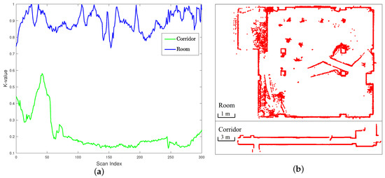
Figure 3. The comparative results of the k-value in different scenes. (a) The k-value in two typical scenes. (b) The corresponding lidar scan maps.

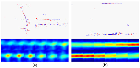
Figure 4. Comparative examples of different scenes. The cost function is visualized with each tile representing a slice of the cost volume for a fixed orientation. Red color represents high cost volume and blue color represents low cost volume. (a) An example with the value of k near $1.0$. (b) An example with a small value of k.

Our improved CSM algorithm utilizes k as the penalty factor $\omega \left(k\right)$ to increase the odometry accuracy by means of motion model $p\left(x_i\right|x_{i-1},u)$ as

$$S_j=S_j+\omega \left(k\right)\Vert {\mathcal{T}}_j-u\Vert ,$$

(9)

where $\Vert {\mathcal{T}}_j-u\Vert$ means the difference between the observation model and the motion model, and ${\mathcal{T}}^{*}$ corresponds to ${\mathcal{T}}_j$ with the maximum score $S_j$. We set $\omega \left(k\right)=\lambda (k-1)$, where $\lambda >0$.

3.2. Loop Closure Detection and Validation

Our loop closure detection and validation method is mainly composed of three parts: Detecting loop closure candidates based on AdaBoost, hierarchically selecting positive loops with high confidence and rejecting false loops according to the residual error from the back-end optimizer. It should be noted that, our method of detecting loop closure candidates is similar to [11]. However, we improve the accuracy of classification by introducing more robust features and decrease the false alarm by several validation steps.

3.2.1. Point Cloud Feature Extraction

Similar to [11], we extract rotation invariant features as follows: (1) Area features: Area, close area; (2) Distance features: Distance, close distance, far distance, average range, centroid, maximum range, mean deviation, standard deviation of range; (3) Shape features: Circularity radius, circularity residual, curvature mean, curvature standard deviation, regularity; (4) Cluster features: Number of groups, mean group size; and (5) Others: Size and mean of angular difference. For detailed definition and formulation of these features, please refer to [11,33]. Based on [11,33], we have improved the feature extraction in three aspects.

(1) Firstly, for the mean and the standard deviation of the curvatures, the original method in [11] only takes three consecutive points into account to calculate the curvature of the middle point, which is sensitive to noise. Let $p_i$ be a point in the lidar cloud $P_k$, and let ${\mathcal{S}}_i$ be the neighboring consecutive point sets of $p_i$. We choose three points on each side of $p_i$, and the smoothness is evaluated as

$$c_i=\frac{1}{|{\mathcal{S}}_i|·\Vert X_{k,i}\Vert }\Vert \sum _{j\in {\mathcal{S}}_i,j\ne i}(X_{k,i}-X_{k,j})\Vert .$$

(10)

The curvature mean $\overline{c}$ and the standard deviation $\sigma \left(c\right)$ are defined as

$$\overline{c}=\frac{1}{N}\sum _{i=1}^N{c}_i,\sigma \left(c\right)=\sqrt{\frac{1}{N-1}\sum _{i=1}^N{(c_i-\overline{c})}^2}.$$

(11)

(2) Secondly, for the number of groups and the mean of group size, rather than using a constant maximum distance to separate consecutive points [11], we adopt an adaptive breakpoint detector as introduced in [34]. The adaptive distance threshold of point $p_i$ is defined as

$$D_{Th}^i=r_i·\frac{\sin (\Delta \phi )}{\sin (\lambda -\Delta \phi )}+3\sigma ,$$

(12)

where $r_i$ is the distance from $p_i$ to the origin of the coordinate, $\Delta \phi$ corresponds to the angle interval of the range scan, $\lambda$ is an empirical value determining the radius of the threshold circle and $\sigma$ corresponds to the measurement accuracy of the laser scanner. A breakpoint is detected when the distance between consecutive points exceeds $D_{Th}^i$. An example is shown in Figure 5, where the black points represent breakpoints and the red point sets between two consecutive breakpoints belong to one cluster.

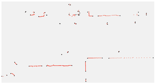
Figure 5. Segmentation results based on the adaptive breakpoint detector. The black points represent breakpoints and the red point sets between two consecutive breakpoints belong to one cluster.

Besides the above two features, we introduce another five-dimensional feature based on the size of the cluster. We discretize the size of the cluster into 5 levels, and calculate the ratio of each level $L=[l_1,l_2,l_3,l_4,l_5]$, where $l_i$ is normalized. We termed this feature as Cluster Distribution Histogram (CDH). The size of each level is set empirically. This five-dimensional feature together with the first two features constitutes the distribution of the point cloud clusters. Three examples of CDH from our real scan data is shown in Figure 6.

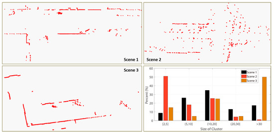
Figure 6. Comparative examples of CHD and their corresponding visualized scans.

(3) Thirdly, we introduce three more features based on scan matching result, including the normalized score of the maximum scan matching alignment, the k-value computed by Equation (7) and the missing rate of query scan points. In particular, the k-value reflects the characteristic of the scene, and the missing rate corresponds to the rate of the query scan points which are projected into the black region of the rasterized cost table as shown in Figure 2.

3.2.2. Classification Based on AdaBoost

All those m rotation invariant features are computed for each scan, defined as ${\mathsf{\Lambda }}^i=[{\lambda }_1^i,{\lambda }_2^i,\cdots ,{\lambda }_m^i],i\in N$, where N corresponds to the total number of scans. Given two laser scans k and l, the set of features for the classifier is defined as

$$\left\{\begin{array}{c}\begin{array}{c}x({\mathsf{\Lambda }}^k,{\mathsf{\Lambda }}^l)=[f_1,f_2,\cdots ,f_m]\hfill \\ f_j=\Vert {\lambda }_j^k-{\lambda }_j^l\Vert ,j\in [1,m].\hfill \end{array}\hfill \end{array}\right.$$

(13)

For the training data, a set of n labeled scan pairs are provided

$$\left(x_1({\mathsf{\Lambda }}^k,{\mathsf{\Lambda }}^l),y_1\right),\left(x_2({\mathsf{\Lambda }}^k,{\mathsf{\Lambda }}^l),y_2\right),\cdots ,\left(x_n({\mathsf{\Lambda }}^k,{\mathsf{\Lambda }}^l),y_n\right),$$

(14)

where $y_i\in \{1,-1\}$ is the label of a sample input indicating matching and nonmatching scan pairs.

AdaBoost is applied as the classifier constituted with a series of weak classifiers. The AdaBoost algorithm is described in Algorithm 3. The algorithm firstly trains a base classifier from the initial training sets, and then adjusts the distribution of the training samples according to the classification error, so that the previously misclassified samples receive more attention in the following step. And then the next weak classifier is trained based on the updated sample distribution. The above two steps are repeated until the maximum iteration T is reached. The final classifier is a weighted combination of T weak classifiers, and these weak classifiers with smaller classification errors have larger weights.

3.2.3. Loop Closure Validation

It is worth noting that one single wrong loop closure can cause severe damage to the whole pose graph. It is necessary to perform validation to eliminate the false loop closures. Our system adopts three strategies to reject false loops:

(1) Firstly, for every positive loop closure detected by the AdaBoost classifier, we calculate the best score of the query scan projected to the coarse raster table, defined as $S_L^{best}$. The candidates detected from the classifier with $S_L^{best}<S_L^{Th}$ are rejected.

(2) Secondly, we calculate the scan matching results at high resolution, including the best score $S_H^{best}$, the k computed by Equation (8) and the missing rate of query scan points defined as $p_{miss}$. Three thresholds are used to select positive loop closures with high confidence.

(3) Thirdly, we perform consistency validation by inverse scan alignment which we named as Direct-Inverse Matching Consistency (DIMC). Unlike local matching algorithms such as ICP and ICL, CSM may produce a large deviation between the direct matching and the inverse matching when two scans belong to a false loop closure. An example from our data is shown in Figure 7, where the blue points belong to the target scan and the red points belong to the source scan. Due to the significant changes in viewpoint, the scan matching result is unreliable, which can be verified through DIMC.

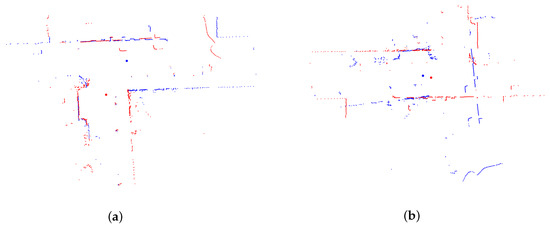
Figure 7. An example of false loop closure detected by DIMC. The blue points belong to the target scan and the red points belong to the source scan. The translation error between (a) and (b) is 2.624 meters. (a) Direct matching result. (b) Inverse matching result.

Algorithm 3 Classifier based on AdaBoost

Require: Training set $\mathcal{D}=\{(x_1,y_1),(x_2,y_2),\cdots ,(x_n,y_n)\},$ Maximum iteration T  1: Initialize the sample weight distribution: ${\omega }_1\left(x\right)=\frac{1}{n}$;  2: for$t=1$ to T do  3:  Train a weak classifier $h_t$ based on ${\omega }_t$:  $h_t=\zeta (\mathcal{D},{\omega }_t);$  4:  Compute classification error of $h_t$:  ${\epsilon }_t=P(h_t\left(x\right)\ne f\left(x\right));$ where $f\left(x\right)$ is the authenticity discriminant function.  5:  if ${\epsilon }_t\ge 0.5$ then  6:   continue;  7:  end if  8:  Compute the weight of the weak classifier $h_t$:  ${\alpha }_t=\frac{1}{2}\ln (\frac{1-{\epsilon }_t}{{\epsilon }_t});$  9:  Update the sample weight distribution:  ${\omega }_{t+1}\left(x\right)=\frac{{\omega }_t\left(x\right)\exp \left(-{\alpha }_{t}f\left(x\right)h_t\left(x\right)\right)}{{\eta }_t};$ where ${\eta }_t$ is the normalization factor. 10: end for 11: $H\left(x\right)=\mathrm{sign}\left({\displaystyle \sum _{t=1}^T}{\alpha }_t{h}_t\left(x\right)\right)$ 12: return$H\left(x\right)$

3.3. Back-End Optimization

The back-end performs graph optimization based on the results generated from the front-end and the loop closure detection, resulting in a consistent trajectory and an optimized map.

The problem can be represented as the Bayesian belief network [25]. The joint probability of the variables is modeled as

$$P\left(X\right|U)\propto \underset{\mathrm{adjacent}\mathrm{constraints}}{\underbrace{\prod _{i}P\left(x_{i+1}\right|x_i,u_i)}}·\underset{\mathrm{loop}\mathrm{closures}}{\underbrace{\prod _{ij}P\left(x_j\right|x_i,u_{ij})}},$$

(15)

where X is the set of nodes and U stands for the set of edges, $P\left(x_{i+1}\right|x_i,u_i)$ is the motion model constructed from adjacent frame constraints given by the front-end, $P\left(x_j\right|x_i,u_{ij})$ corresponds to the measurement model generated from loop closure detections.

The state transformation model corresponding to $P\left(x_{i+1}\right|x_i,u_i)$ is defined as

$$x_{i+1}=f_{i,i+1}(x_i,u_i)+w_{i,i+1},$$

(16)

where $f_{i,i+1}(·)$ is the state transformation function, $w_{i,i+1}$ is the Gaussian noise with zero-mean and covariance ${\sum }_i$. Similarly, the state transformation model corresponding to $P\left(x_j\right|x_i,u_{ij})$ is defined as

$$x_j=f_{i,j}(x_i,u_{ij})+w_{i,j},$$

(17)

and the covariance of $w_{i,j}$ is ${\mathsf{\Lambda }}_{ij}$. Combining ((15),(16),(17)), the maximum-a-posteriori estimation can be formed into a nonlinear optimization problem

$$\begin{array}{cc}\hfill X^{*}& =\arg \underset{X}{\max }P\left(X\right|U)\hfill \\ & =\arg \underset{X}{\min }\underset{\mathrm{adjacent}\mathrm{constraints}}{\underbrace{\sum _i{\Vert f(x_i,u_i)-x_{i+1}\Vert }_{{\sum }_i}^2}}+\underset{\mathrm{loop}\mathrm{closures}}{\underbrace{\sum _{ij}{\Vert f(x_i,u_{ij})-x_j\Vert }_{{\mathsf{\Lambda }}_{ij}}^2}},\hfill \end{array}$$

(18)

where ${\Vert e\Vert }_{\sum }^2=e^T{\sum }^{-1}e$.

As described in [25], the above nonlinear optimization problem can be transformed into the standard least squares problem based on Gauss-Newton or Levenberg-Marquardt algorithm

$$X^{*}=\arg \underset{X}{\min }{\Vert AX-b\Vert }^2,$$

(19)

where $X\in {\mathbb{R}}^n$ contains all pose variables, the sparse measurement matrix $A\in {\mathbb{R}}^{m\times n}$ contains all edges, and $b\in {\mathbb{R}}^m$ is the right hand side (RHS) vector corresponding to the difference between the estimated state and the measurement vector.

Different from the work in [25], we improved the back-end mainly in two aspects.

(1) Firstly, the covariance matrix computed in Equation (6) can be embedded into the above optimization framework as an adaptive information matrix. This will ensure that edges with strong confidence are not prone to be adjusted during the optimization procedure, whilst edges with low confidence are more likely to be tuned.

(2) Secondly, our system rejects false loops according to the residual error from the back-end optimizer. The residual error is computed between trajectories before and after the optimization. A large difference indicates a high likelihood of false loops.

4. Experiments and Results

During our experiments, the algorithms run on a laptop computer with 2.4 GHz Intel Core i7 CPU and 8 GB of RAM. In order to achieve real-time performance, multiple CPU threads are utilized in parallel. We perform experiments both on the data collected by our own platform and also on KITTI benchmark. Our platform is a golf cart equipped with a Velodyne VLP-16, a wheel encoder and a low cost IMU, as shown in Figure 8. Although VLP-16 produces 16 scanning lines, we only utilize one single horizontal scanning line to mimic a 2D lidar. The same method is also applied on the KITTI datasets.

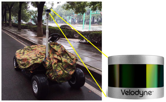
Figure 8. Our platform and lidar sensor.

4.1. The Results of the Improved Correlative Scan Matcher

For the first experiment, we perform the simple laser scan alignment without loop closure detection or back-end optimization to validate the improvement of our front-end method. The comparative results of the original CSM and our improved CSM are shown in Figure 9. The translation errors are evaluated following the KITTI’s protocol with lengths (100 m, 200 m, ⋯, 800 m) in 2D coordinates [32].

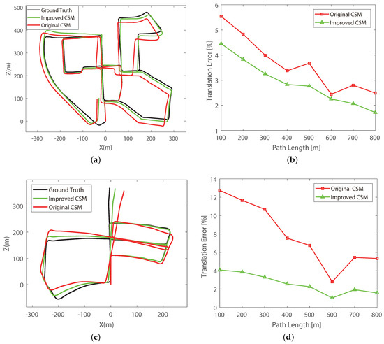
Figure 9. Results of the odometry estimation with only the front-end. (a) Trajectories of the 0th sequence. (b) Translation errors of the 0th sequence. (c) Trajectories of the 5th sequence. (d) Translation errors of the 5th sequence.

As shown in Figure 9, the trajectories of our improved CSM are closer to the ground truth than those of the original CSM in both the 0th sequence and the 5th sequence. While the average running time of our improved CSM increases by less than 0.01 s.

4.2. The Results of Loop Closure Detection and Validation

As described in Section 3.2, the loop closure classifier based on AdaBoost is trained from our dataset campus $\#1$. The dataset is collected around the campus covering an area of 1750 m × 910 m while traveling around 15.99 kilometers with 22,935 scans. We choose 2000 matching and 2000 nonmatching laser pairs which are pre-labeled to train the classifier by 10-fold cross validation.

We choose three other approaches for comparison: Method 1 [11] is the most similar one to our method, and the main difference is that we utilize more features as described in Section 3.2; method 2 is based on Support Vector Machine (SVM) using the same features as our method; method 3 is based on deep learning algorithm similar to [13]. Figure 10 shows the precision-recall curves for all these three approaches together with our proposed approach.

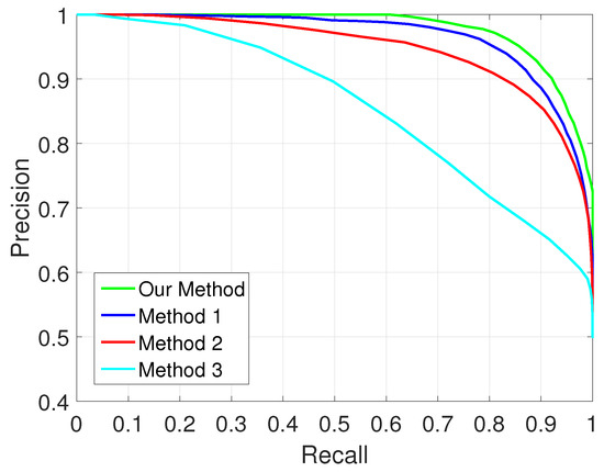
Figure 10. Precision-recall curves for the results of loop closure detection.

Compared with method 1, our algorithm performs better on the campus $\#1$ dataset. A threshold of $K=0.3$ gives a detection rate of $92.6\%$ and a false alarm rate of $2.7\%$. Although the false alarm rate of our method is a bit higher than method 1, it will be further reduced through validation (DIMC) and false loop closure rejection based on the back-end optimization. The subsequent experiments will show that our system can achieve nearly $0\%$ false alarm for different types of datasets. Method 3 achieves the worst performance on our dataset. The main reason is that the dataset tested in [13] is a much smaller dataset collected in structured indoor environment whilst our campus $\#1$ dataset is built in large-scale outdoor environment.

For time complexity, our method outperforms method 1 both in feature extraction and classification, as shown in Table 1.

Table 1. Time performance of loop closure detection.

Method	Time Consumption
	Feature Extraction	Classification
Method 1	19 ms	2 ms
Our Method	100 us	42 us

During all the experiments including fifteen datasets from campus $\#1$, one dataset from the Zhongdian Science and Technology Park and eleven datasets from KITTI benchmark, only two false loop closures are rejected according to the residual error from the back-end optimizer. Our loop closure detection and validation algorithm performs consistently well.

4.3. Test with Our Datasets

Figure 11 shows the mapping of campus $\#1$ area, where the map (shown in red dots) is projected onto a satellite image. The map shows a good consistency with the satellite image. Besides campus $\#1$, we also test our 2D-SLAM system on several other datasets including a dataset from the Zhongdian Science and Technology Park as shown in Figure 12. Results indicate that our system works consistently well in large-scale outdoor environment. Figure 13 shows a snapshot of our mapping process. The red points are obstacles mapped online; the blue points represent the current laser scan; the green points represent the vehicle trajectory and the dark yellow lines are the loop closures. The current vehicle pose is shown as the yellow arrow.

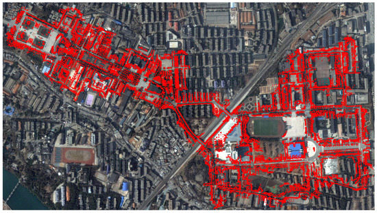
Figure 11. Mapping of the campus $\#1$ area.

Figure 12. Mapping of the Zhongdian Science and Technology Park.

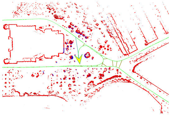
Figure 13. The mapping process visualization. The red points are obstacles mapped online; the blue points represent the current laser scan; the green points represent the vehicle trajectory and the dark yellow lines are the loop closures.

We qualitatively compare our method with a state-of-the-art 2D SLAM algorithm: Cartographer [12]. Figure 14 shows the trajectories generated by our method and cartographer. As can be seen from Figure 14, our method can compete with cartographer in terms of accuracy. For computational efficiency, our method built the whole map in 27.54 minutes compared with 31.09 min for cartographer. Detailed comparisons of these two approaches are shown in Figure 15, where scenes $\#1$, $\#2$ and $\#3$ are labeled in Figure 14. For scene $\#1$, cartographer generates a wrong loop closure which results in blurry lines at place A. As for our map rendering step applies dynamic objects filtering borrowed from Wang et al. [35], the unreliable points are filtered effectively. The different results can be seen from B and C in scene $\#1$, A and B in scene $\#2$ as well as C in scene $\#3$. Place C in scene $\#2$ along with A and B in scene $\#3$ indicate that our map contains richer details with less noise than cartographer.

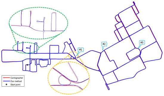
Figure 14. Comparison of trajectories between cartographer and our method.

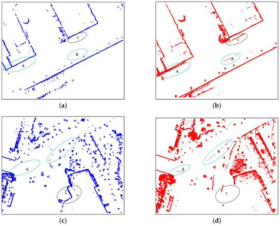
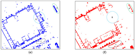
Figure 15. Comparison of mapping details from different methods. (a) Our map of scene $\#1$. (b) Cartographer’s map of scene $\#1$. (c) Our map of scene $\#2$. (d) Cartographer’s map of scene $\#2$. (e) Our map of scene $\#3$. (f) Cartographer’s map of scene $\#3$.

4.4. Test with KITTI Datasets

Our system has also been tested on the large-scale and publicly available KITTI datasets, and the experimental results are shown in Figure 16. To mimic the 2D laser setting, we extract one single laser scan of the Velodyne HDL-64 lidar. Due to space issue, we present results of two typical sequences (Sequences 13 and 15). We choose LOAM, ICP and NDT as the comparison approaches. ICP and NDT are widely used scan matching approaches in lidar SLAM system. LOAM is ranked $\#1$ among all lidar based methods on KITTI dataset.

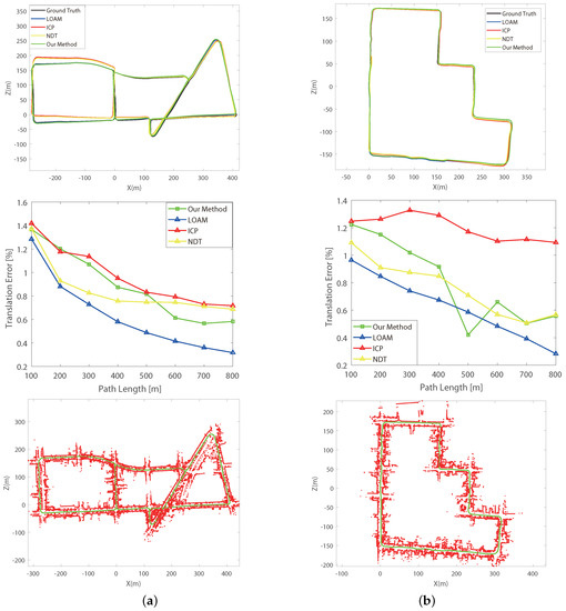
Figure 16. Paths and mapping results from the KITTI datasets. (a) Scequence 13. (b) Scequence 15.

It is worth mentioning that all these comparison approaches are based on the whole 3D lidar data, whilst our approach only utilizes one single scanning line of the 3D lidar. As shown in Figure 16, the experimental results indicate that our system achieves comparable performance compared to other benchmark approaches. It is worth mentioning that sequence 13 is prone to false loop closures around the viaduct due to the limitation of 2D framework. However, our system can detect and eliminate these wrong loops successfully. For computational efficiency, our system achieves a superior runtime of 0.06 s per scan compared with 0.1 s of LOAM.

5. Concluding Remarks

In this paper, a robust 2D lidar SLAM system for large-scale outdoor environment is proposed. To improve the accuracy and robustness of scan matching, an extension to the CSM is proposed. For efficient place recognition, an AdaBoost based loop closure detection is proposed. We also propose a light-weight back-end optimization algorithm that works in real-time. The optimization results are also utilized to eliminate false loop closures. Experiments both on our own collected dataset and the publicly available KITTI dataset confirmed the effectiveness of our approach. For the future work, we would like to apply our method to 3D mapping and localization. Moreover, the implementation of our map for localization on different platforms will be verified in our further work.

References

- Cadena, C.; Carlone, L.; Carrillo, H.; Latif, Y.; Scaramuzza, D.; Neira, J.; Reid, I.; Leonard, J.J. Past, Present, and Future of Simultaneous Localization and Mapping: Toward the Robust-Perception Age. IEEE Trans. Robot. 2016, 32, 1309–1332. [Google Scholar] [CrossRef]
- Rusinkiewicz, S.; Levoy, M. Efficient variants of the ICP algorithm. In Proceedings of the Third International Conference on 3-D Digital Imaging and Modeling, Quebec City, CA, USA, 28 May–1 June 2001; pp. 145–152. [Google Scholar] [CrossRef]
- Biber, P.; Strasser, W. The normal distributions transform: a new approach to laser scan matching. In Proceedings of the 2003 IEEE/RSJ International Conference on Intelligent Robots and Systems (IROS 2003) (Cat. No.03CH37453), Las Vegas, NV, USA, 27–31 October 2003; Volume 3, pp. 2743–2748. [Google Scholar] [CrossRef]
- Olson, E.B. Real-time correlative scan matching. In Proceedings of the 2009 IEEE International Conference on Robotics and Automation, Kobe, Japan, 12–17 May 2009; pp. 4387–4393. [Google Scholar] [CrossRef]
- Chong, Z.J.; Qin, B.; Bandyopadhyay, T.; Ang, M.H.; Frazzoli, E.; Rus, D. Mapping with synthetic 2D LIDAR in 3D urban environment. In Proceedings of the 2013 IEEE/RSJ International Conference on Intelligent Robots and Systems, Tokyo, Japan, 3–8 November 2013; pp. 4715–4720. [Google Scholar] [CrossRef]
- Olson, E. M3RSM: Many-to-many multi-resolution scan matching. In Proceedings of the 2015 IEEE International Conference on Robotics and Automation (ICRA), Seattle, WA, USA, 26–30 May 2015; pp. 5815–5821. [Google Scholar] [CrossRef]
- Gao, X.; Wang, R.; Demmel, N.; Cremers, D. LDSO: Direct Sparse Odometry with Loop Closure. In Proceedings of the 2018 IEEE/RSJ International Conference on Intelligent Robots and Systems (IROS), Madrid, Spain, 1–5 October 2018; pp. 2198–2204. [Google Scholar] [CrossRef]
- Galvez-López, D.; Tardos, J.D. Bags of Binary Words for Fast Place Recognition in Image Sequences. IEEE Trans. Robot. 2012, 28, 1188–1197. [Google Scholar] [CrossRef]
- Engel, J.; Koltun, V.; Cremers, D. Direct Sparse Odometry. IEEE Trans. Pattern Anal. Mach. Intell. 2018, 40, 611–625. [Google Scholar] [CrossRef] [PubMed]
- Mur-Artal, R.; Tardós, J.D. ORB-SLAM2: An Open-Source SLAM System for Monocular, Stereo, and RGB-D Cameras. IEEE Trans. Robot. 2017, 33, 1255–1262. [Google Scholar] [CrossRef]
- Granstrom, K.; Callmer, J.; Ramos, F.; Nieto, J. Learning to detect loop closure from range data. In Proceedings of the 2009 IEEE International Conference on Robotics and Automation, Kobe, Japan, 12–17 May 2009; pp. 15–22. [Google Scholar] [CrossRef]
- Hess, W.; Kohler, D.; Rapp, H.; Andor, D. Real-time loop closure in 2D LIDAR SLAM. In Proceedings of the 2016 IEEE International Conference on Robotics and Automation (ICRA), Stockholm, Sweden, 16–21 May 2016; pp. 1271–1278. [Google Scholar] [CrossRef]
- Li, J.; Zhan, H.; Chen, B.M.; Reid, I.; Lee, G.H. Deep learning for 2D scan matching and loop closure. In Proceedings of the 2017 IEEE/RSJ International Conference on Intelligent Robots and Systems (IROS), Vancouver, BC, Canada, 24–28 September 2017; pp. 763–768. [Google Scholar] [CrossRef]
- Xue, H.; Fu, H.; Dai, B. IMU-Aided High-Frequency Lidar Odometry for Autonomous Driving. Appl. Sci. 2019, 9, 1506. [Google Scholar] [CrossRef]
- Alshawa, M. ICL: Iterative closest line a novel point cloud registration algorithm based on linear features. Ekscentar 2007, 10, 53–59. [Google Scholar]
- Zhang, J.; Singh, S. Low-drift and real-time lidar odometry and mapping. Auton. Robots 2017, 41, 401–416. [Google Scholar] [CrossRef]
- Censi, A.; Iocchi, L.; Grisetti, G. Scan Matching in the Hough Domain. In Proceedings of the 2005 IEEE International Conference on Robotics and Automation, Barcelona, Spain, 18–22 April 2005; pp. 2739–2744. [Google Scholar] [CrossRef]
- Rofer, T. Using histogram correlation to create consistent laser scan maps. In Proceedings of the IEEE/RSJ International Conference on Intelligent Robots and Systems, Lausanne, Switzerland, 30 September–4 October 2002; Volume 1, pp. 625–630. [Google Scholar] [CrossRef]
- Bosse, M.; Roberts, J. Histogram Matching and Global Initialization for Laser-only SLAM in Large Unstructured Environments. In Proceedings of the 2007 IEEE International Conference on Robotics and Automation, Roma, Italy, 10–14 April 2007; pp. 4820–4826. [Google Scholar] [CrossRef]
- Fox, D.; Burgard, W.; Dellaert, F.; Thrun, S. Monte Carlo localization: Efficient position estimation for mobile robots. In Proceedings of the Sixteenth National Conference on Artificial Intelligence and Eleventh Conference on Innovative Applications of Artificial Intelligence, Orlando, FL, USA, 18–22 July 1999; pp. 343–349. [Google Scholar]
- Grisetti, G.; Stachniss, C.; Burgard, W. Improved Techniques for Grid Mapping With Rao-Blackwellized Particle Filters. IEEE Trans. Robot. 2007, 23, 34–46. [Google Scholar] [CrossRef]
- Bosse, M.; Zlot, R. Map Matching and Data Association for Large-Scale Two-dimensional Laser Scan-based SLAM. Int. J. Robot. Res. 2008, 27, 667–691. [Google Scholar] [CrossRef]
- Himstedt, M.; Frost, J.; Hellbach, S.; Böhme, H.; Maehle, E. Large scale place recognition in 2D LIDAR scans using Geometrical Landmark Relations. In Proceedings of the 2014 IEEE/RSJ International Conference on Intelligent Robots and Systems, Chicago, IL, USA, 14–18 September 2014; pp. 5030–5035. [Google Scholar] [CrossRef]
- Tipaldi, G.D.; Arras, K.O. FLIRT-Interest regions for 2D range data. In Proceedings of the 2010 IEEE International Conference on Robotics and Automation, Anchorage, AK, USA, 3–7 May 2010; pp. 3616–3622. [Google Scholar] [CrossRef]
- Kaess, M.; Ranganathan, A.; Dellaert, F. iSAM: Incremental Smoothing and Mapping. IEEE Trans. Robot. 2008, 24, 1365–1378. [Google Scholar] [CrossRef]
- Kaess, M.; Johannsson, H.; Roberts, R.; Ila, V.; Leonard, J.; Dellaert, F. iSAM2: Incremental smoothing and mapping with fluid relinearization and incremental variable reordering. In Proceedings of the 2011 IEEE International Conference on Robotics and Automation, Shanghai, China, 9–13 May 2011; pp. 3281–3288. [Google Scholar] [CrossRef]
- Kümmerle, R.; Grisetti, G.; Strasdat, H.; Konolige, K.; Burgard, W. G2o: A general framework for graph optimization. In Proceedings of the 2011 IEEE International Conference on Robotics and Automation, Shanghai, China, 9–13 May 2011; pp. 3607–3613. [Google Scholar] [CrossRef]
- Roy, N.; Newman, P.; Srinivasa, S. Inference on Networks of Mixtures for Robust Robot Mapping. In Robotics: Science and Systems VIII; The MIT Press: Cambridge, MA, USA, 2013. [Google Scholar]
- Sünderhauf, N.; Protzel, P. Towards a robust back-end for pose graph SLAM. In Proceedings of the 2012 IEEE International Conference on Robotics and Automation, Saint Paul, MN, USA, 14–18 May 2012; pp. 1254–1261. [Google Scholar] [CrossRef]
- Latif, Y.; Cadena, C.; Neira, J. Realizing, reversing, recovering: Incremental robust loop closing over time using the iRRR algorithm. In Proceedings of the 2012 IEEE/RSJ International Conference on Intelligent Robots and Systems, Vilamoura, Portugal, 7–12 October 2012; pp. 4211–4217. [Google Scholar] [CrossRef]
- Sünderhauf, N.; Protzel, P. Switchable constraints vs. max-mixture models vs. RRR—A comparison of three approaches to robust pose graph SLAM. In Proceedings of the 2013 IEEE International Conference on Robotics and Automation, Karlsruhe, Germany, 6–10 May 2013; pp. 5198–5203. [Google Scholar] [CrossRef]
- Geiger, A.; Lenz, P.; Urtasun, R. Are we ready for autonomous driving? The KITTI vision benchmark suite. In Proceedings of the 2012 IEEE Conference on Computer Vision and Pattern Recognition, Providence, RI, USA, 16–21 June 2012; pp. 3354–3361. [Google Scholar] [CrossRef]
- Tatistical, S.; Ancouver, S.A.V.; Jones, P.M. Robust Real-time Object Detection. Int. J. Comput. Vis. 2001, 57, 137–154. [Google Scholar]
- Borges, G.A.; Aldon, M. Line Extraction in 2D Range Images for Mobile Robotics. J. Intell. Robot. Syst. 2004, 40, 267–297. [Google Scholar] [CrossRef]
- Wang, D.Z.; Posner, I.; Newman, P. Model-free detection and tracking of dynamic objects with 2D lidar. Int. J. Robot. Res. 2015, 34, 1039–1063. [Google Scholar] [CrossRef]
© 2019 by the authors. Licensee MDPI, Basel, Switzerland. This article is an open access article distributed under the terms and conditions of the Creative Commons Attribution (CC BY) license (http://creativecommons.org/licenses/by/4.0/).