Rollover-Free Path Planning for Off-Road Autonomous Driving

Abstract

Perception, planning, and control are three enabling technologies to achieve autonomy in autonomous driving. In particular, planning provides vehicles with a safe and collision-free path towards their destinations, accounting for vehicle dynamics, maneuvering capabilities in the presence of obstacles, traffic rules, and road boundaries. Existing path planning algorithms can be divided into two stages: global planning and local planning. In the global planning stage, global routes and the vehicle states are determined from a digital map and the localization system. In the local planning stage, a local path can be achieved based on a global route and surrounding information obtained from sensors such as cameras and LiDARs. In this paper, we present a new local path planning method, which incorporates a vehicle’s time-to-rollover model for off-road autonomous driving on different road profiles for a given predefined global route. The proposed local path planning algorithm uses a 3D occupancy grid and generates a series of 3D path candidates in the s-p coordinate system. The optimal path is then selected considering the total cost of safety, including obstacle avoidance, vehicle rollover prevention, and comfortability in terms of path smoothness and continuity with road unevenness. The simulation results demonstrate the effectiveness of the proposed path planning method for various types of roads, indicating its wide practical applications to off-road autonomous driving.

1. Introduction

Autonomous driving has had strong potential in the field of industry in recent years, and the technique has been improved since the late 1990s. In 1997, Demonstrations on California highways proved that autonomous cars can drive on a highway with magnets. Currently, Tesla has equipped its Model S car with a self-driving system, the “autopilot system”. With the improvement of the autonomous driving system, more challenges show up for autonomous vehicles in real-time problems, particularly for off-road autonomous driving with road unevenness [1,2,3].

Perception, planning, and control are three critical components in autonomous vehicles [4,5]. Especially, the planning part makes the vehicle able to decide the path itself [6]. A path planning [7] algorithm for autonomous driving is usually divided into global and local stages. In the global stage, a global route and vehicle states are determined through information from a digital map and a localization system. In the local stage, local paths can be generated to avoid collisions based on the global route and surrounding information from sensors such as LiDARs and cameras. The study of this paper focuses on local path planning methods for vehicles on a predefined uneven global route. In recent years, there have many studies that focused on local path generation. These studies can be categorized into the following three types of approaches: sampling-based approaches, potential-field approaches and grid-based approaches, and discrete optimization approaches.

Sampling-based approaches construct a collision-free path from the initial place to the destination by sampling the configuration that describes the positions and orientations of the vehicle. Typical examples of sampling-based approaches include rapidly exploring random tree (RRT) and RRT variants that are widely used in nonholonomic motion planning [8]. RRTs are incrementally constructed in a manner that the expected distance from a randomly-chosen point to the tree is quickly reduced. However, RRT-based local path planning algorithms for real-time implementations require efficient guiding heuristics for the sampling configuration.

Potential-field approaches assign repulsive forces to obstacles and attractive forces to the goal position virtually, building a potential field for the area from the vehicle to the goal position. A local path can be built along the steepest gradient of the potential field [9]. However, this algorithm can be trapped in local minima of the potential field, and the steepest gradient path is not guaranteed to achieve the goal position.

Grid-based approaches use a set of cells to map the environment. Each cell represents either an empty space or an obstacle at that position in the environment. Within such environment representation, it can be formulated as an optimization problem to find the globally-optimal path that connects each cell from an initial position to the goal position while avoiding obstacles, and many optimization algorithms can be applied [10].

Discrete optimization approaches have achieved huge success in recent years in the field of autonomous vehicles. In this type of algorithm, a finite set of paths is computed by the numerical integration of differential equations that describe the vehicle motion. From this set, an optimal path that has the minimal cost is selected. The idea of using a finite set of paths can greatly reduce the solution space and enable real-time implementation through fast computation [11].

In past decades, there have been many research works concentrating on the highway path planning field, and many 2D local path planning methods were built on this model. However, there is barely no research on local path planning in off-road autonomous driving [12]. Although there were recently some related works focusing on off-road path planning in wheeled robots such as “Robot navigation in cross-country environments” [13], in legged robots such as the “BigDog, the rough-terrain quadruped robot” [14,15], and in tracked robots such as “A novel traveling wave piezoelectric actuated tracked mobile robot utilizing friction effect” [16], to the best of our acknowledge, this is the first work considering rollover-free local path planning in off-road autonomous driving.

In this paper, we propose a local path planning approach, which is a type of discrete optimization approach (DOA) for off-road autonomous driving. Compared to RRT algorithms, DOA algorithms do not have to acquire efficient guiding heuristics, which are more suitable and have a better performance on real-time path planning in autonomous driving. While most path planning approaches have been proposed for highway autonomous driving, there has been relatively little path planning discussion for off-road situations. Compared to the highway autonomous driving, the major challenges of off-road autonomous driving are that the road could be uneven and the obstacles’ size, e.g., heights or depths, can be varied. Some obstacles must be avoided for collision and/or rollover avoidance, while others might be able to safely pass through such as a small falling tree or a small rock. To address this challenge, the off-road path planning approach we proposed in this paper takes the collision avoidance, the pass angle, and the vehicle rollover condition into consideration to enhance both comfortability and safety in off-road autonomous driving. In particular, vehicle rollover models, known as time-to-rollover (TTR) models [17], are seamlessly incorporated for path planning, serving as the basis for rollover warning and avoidance. To generate path candidates, a $s-\rho$ coordinate system, where s is arc length and $\rho$ is the offset distance, is utilized, and the directional information for the global route is blended with the maneuvering of the vehicle by adjusting the lateral offset to the baseline [18]. Overall, this paper has the following contributions:

• To the best of our knowledge, this paper is the first time the vehicle rollover model has been introduced into path planning for off-road autonomous driving to enhance its safety.
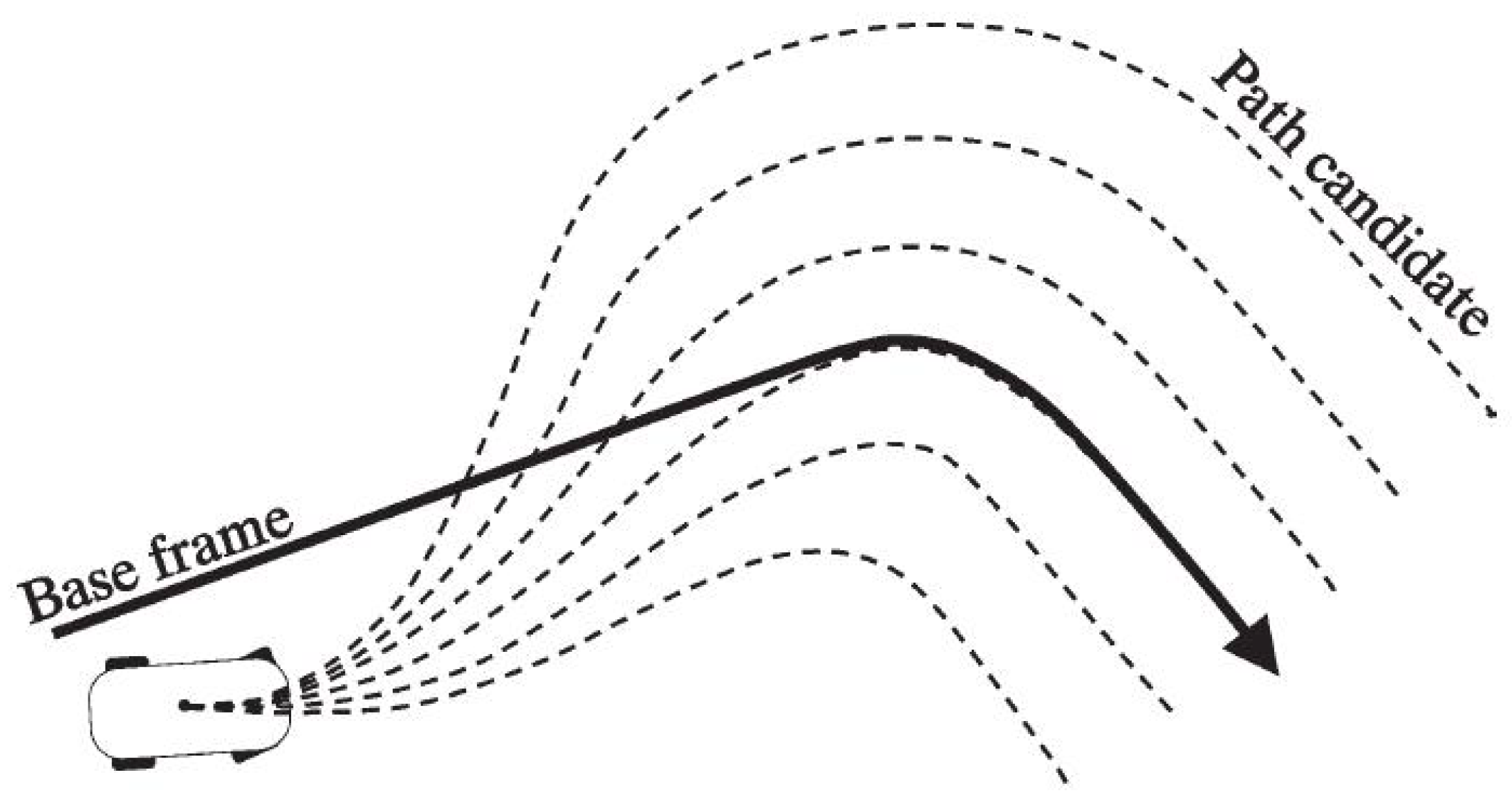
• A path generation method is developed to generate a set of 3D path candidates following the off-road baseline.
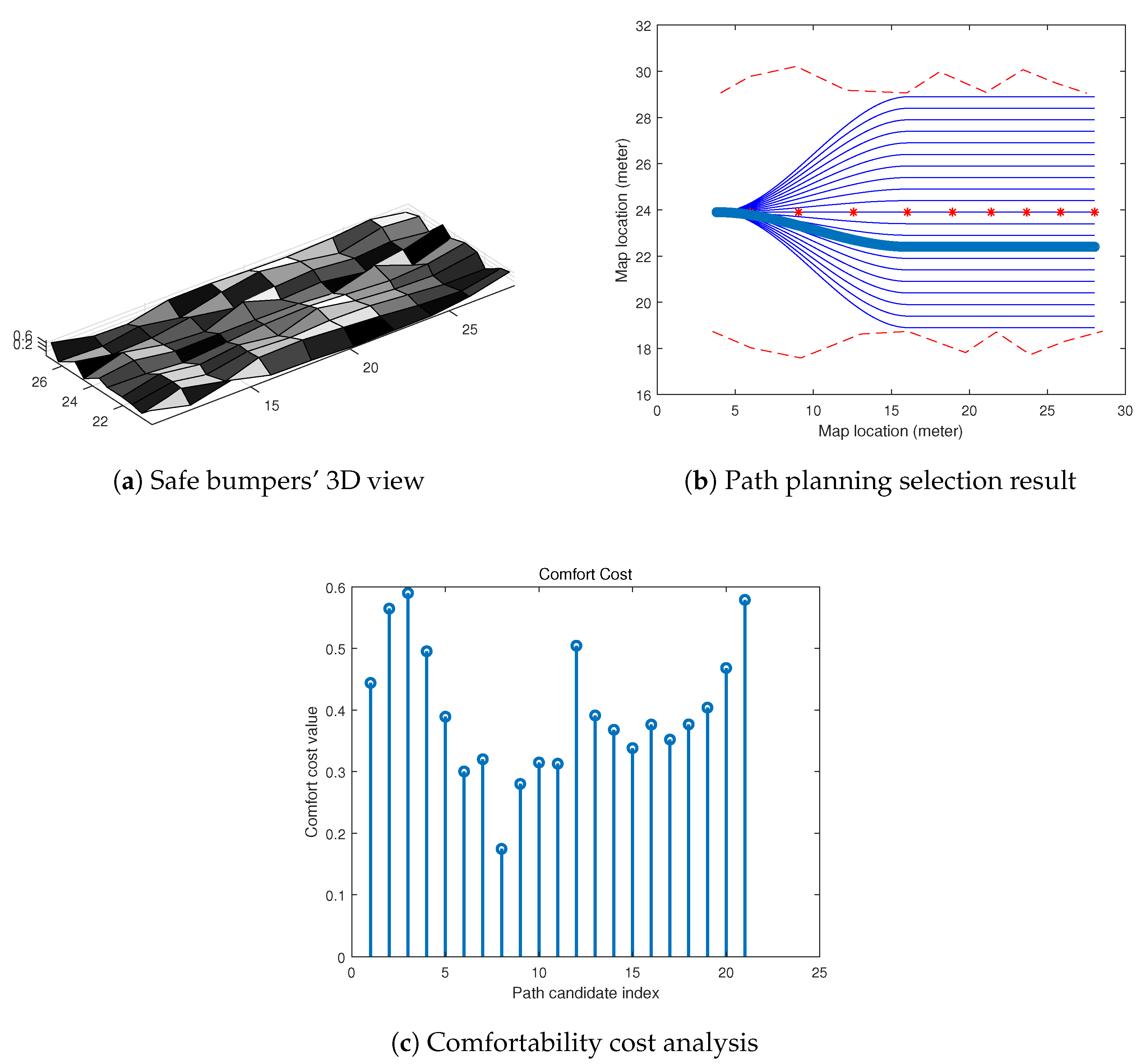
• For each path candidate, a cost function to measure its driving comfortability is proposed with the consideration of road unevenness and path curvature.
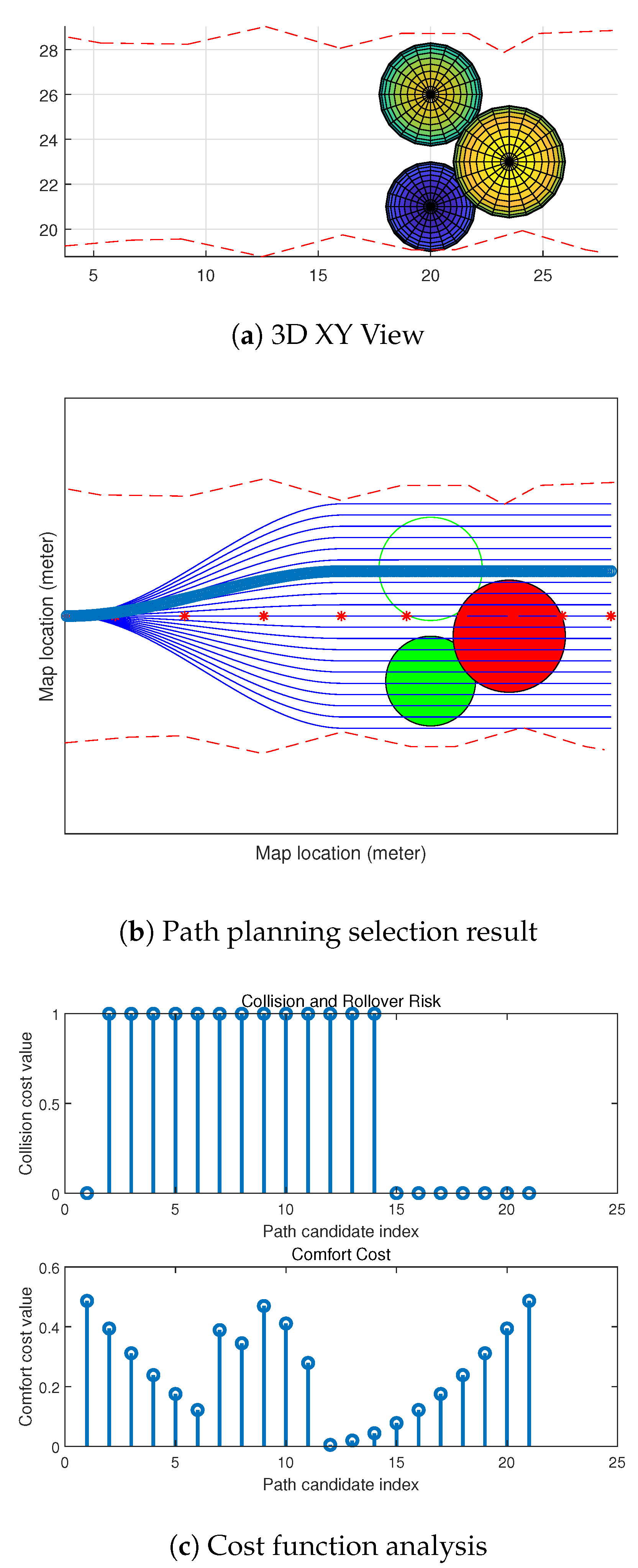
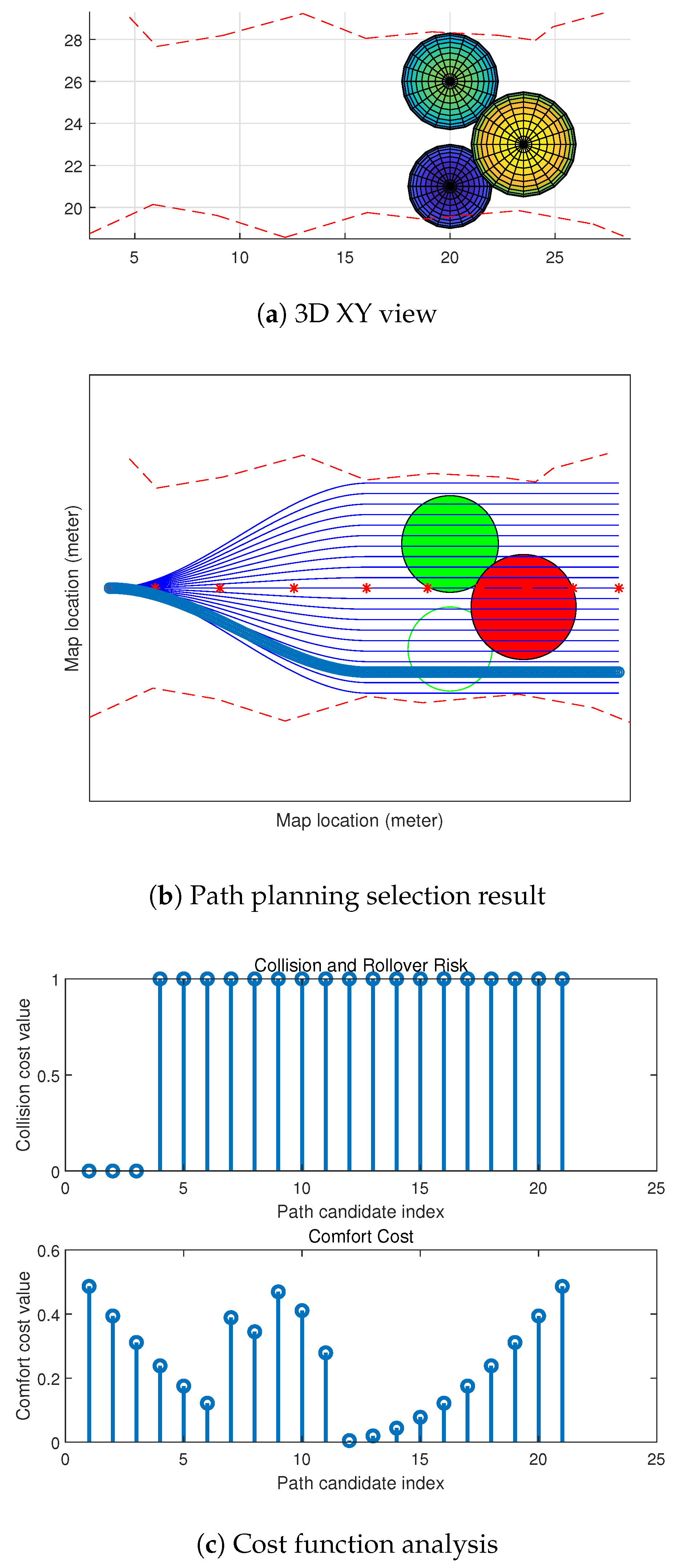
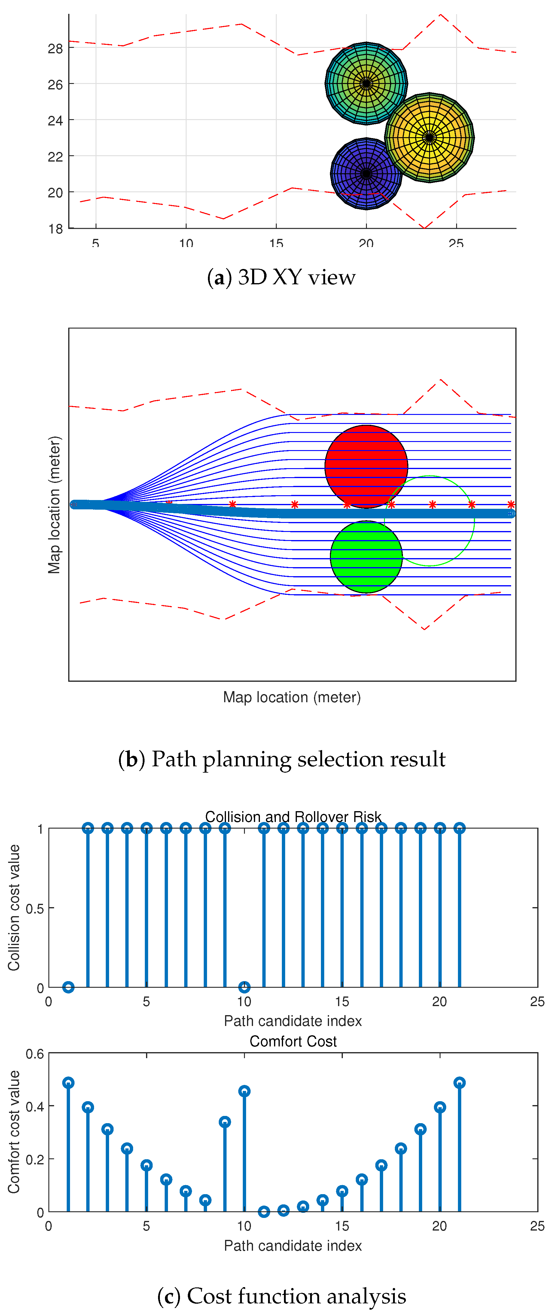
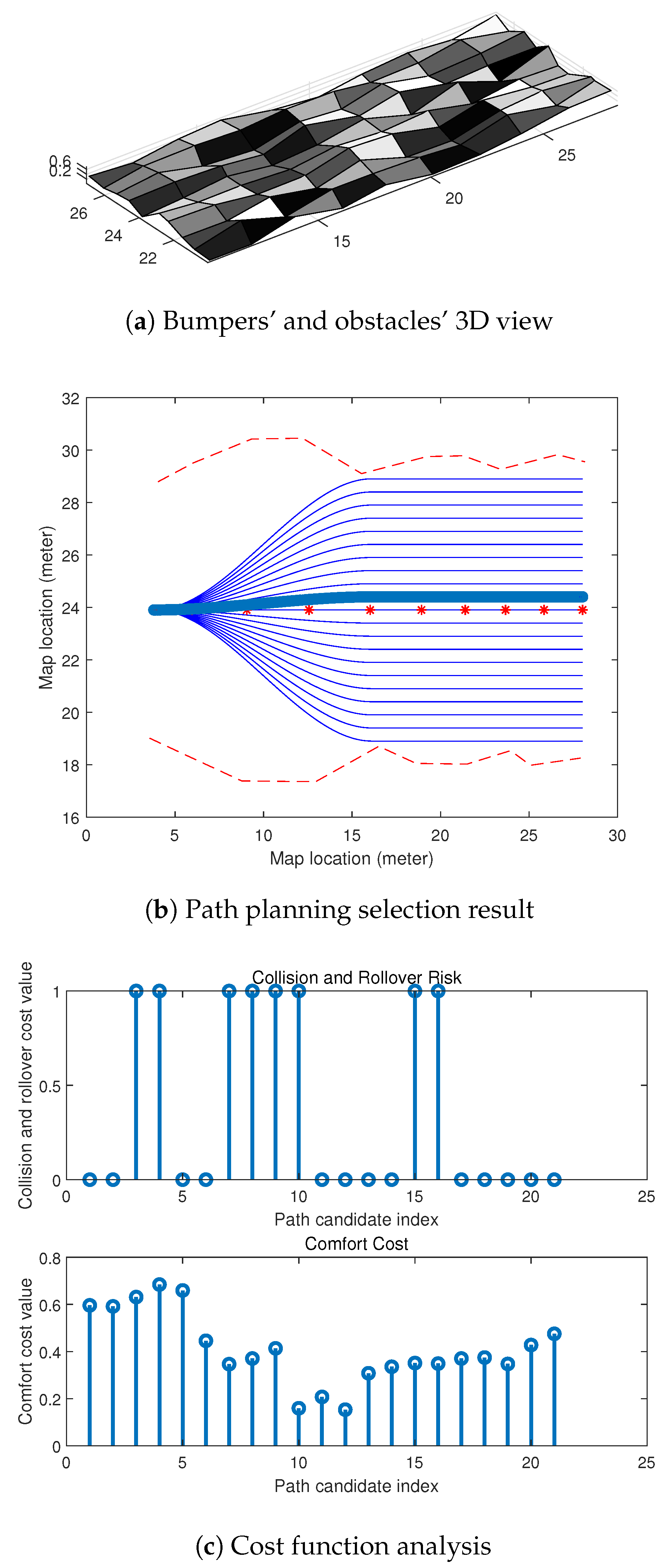
• A cascaded path selection algorithm is developed in this paper to select the optimal path candidate in terms of rollover-free and collision-free safety and comfortability.

The remainder of this paper is organized as follows. Section 2 describes the vehicle rollover challenge for off-road driving and TTR models for rollover avoidance purposes. Section 3 presents the path planning framework, which incorporates TTR models for path selection. Section 4 gives the details of the computational simulations and experimental results. Section 5 concludes the proposed off-road path planning approach and discusses our future work.

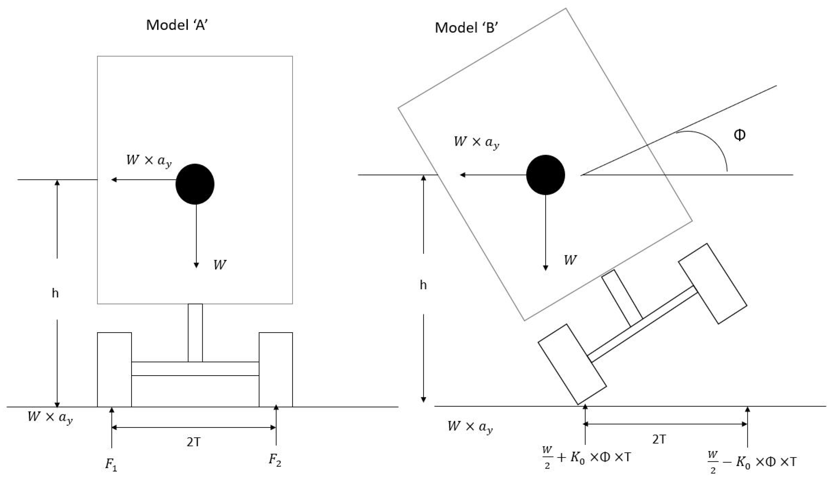
2. Time-to-Rollover Model

A major concern for autonomous driving is to drive safely with the goal of reducing the probability of accidents. In the autonomous driving literature, two types of techniques that can predict vehicle motions for accident avoidance have been widely used [19]: the time-to-collision (TTC) and time-to-lane-crossing (TLC) models. For off-road autonomous driving, this paper introduces the TTR (i.e., time-to-rollover) model to further enhance the safety of autonomous driving with the incorporation of 3D mapping information around the vehicle [20].

2.1. Introduction to the Time-To-Rollover Model

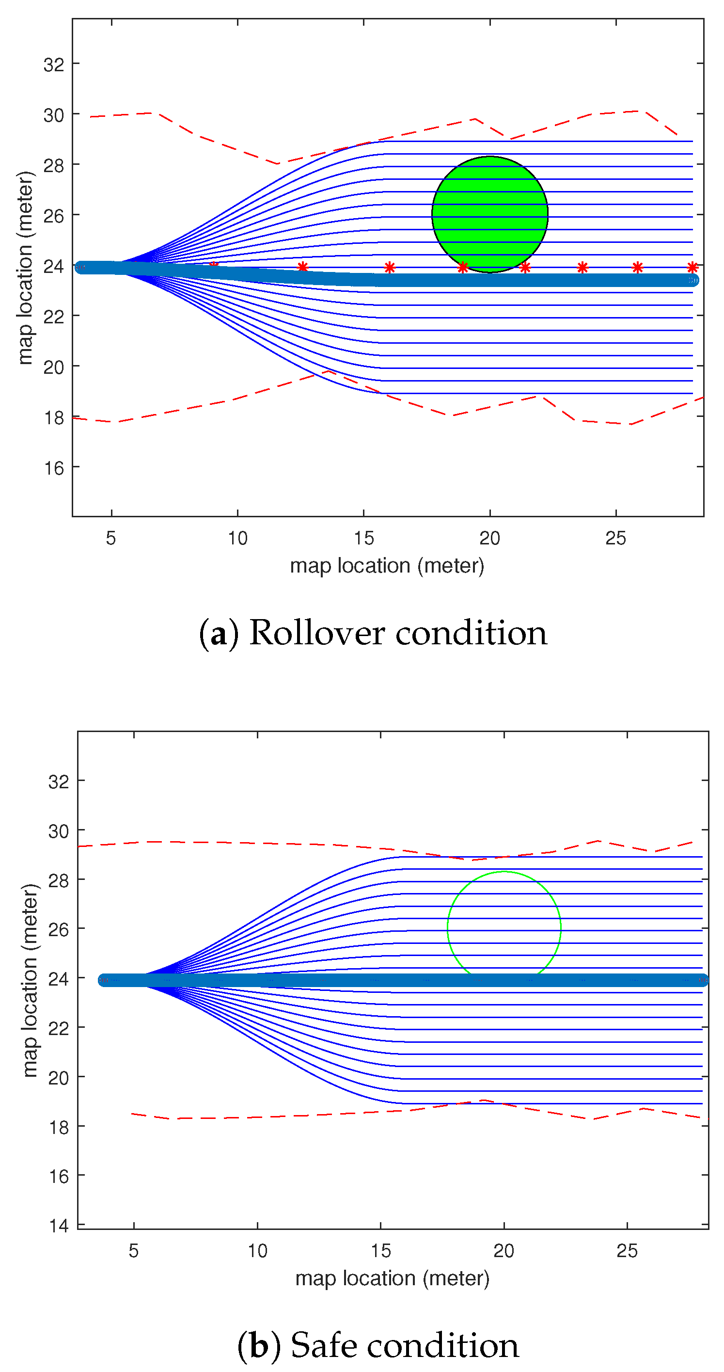
In the U.S., thousands of people are killed in road accidents every year. Among those accidents, records from the National Highway Traffic Safety Administration [21] show that 90% of the harmful events of non-crash accidents are caused by rollover. For off-road driving, there is a higher potential for rollover accidents, considering the uneven road with different types of obstacles or slopes, which are usually not considered in highway driving.

The boundary condition for a vehicle rollover is that tire lift-off happens, which we need to predict and avoid in the path planning algorithms for off-road autonomous driving. The “time-to-rollover” model is thus also known as the “time-to-tire-lift-off” [22]. For a given vehicle’s physical model (e.g., size and tire pressure) and its current states (e.g., orientation and speed), as well as its surrounding environment (e.g., obstacle/hole size and slope), we can compute the time that it takes for the vehicle to reach the rollover boundary condition, i.e., the critical rollover angle.

2.2. Rollover Model

In this paper, we employ the simple rollover with the consideration of both stiffness and rigid suspension of the vehicle [23,24]. The input of the simple rollover model is the steering angle, while other inputs, such as the driver’s braking and road superelevation, are neglected. Two important rollover condition measurements, including the roll angle and roll rate of the vehicle, are output in this rollover model. Figure 1 shows the configuration of two rollover models, in which Model “A” (also known as zero degrees of freedom (DoF)) is a single-unit rigid vehicle without the consideration of tire compliance and Model “B” includes tire compliance producing a 1DOF model. In Model A, the autonomous vehicle’s tractor and trailer are lumped into one unit, which will lift-off at $\varphi$ equal to zero when there is a vertical force. To predict the rollover of a vehicle that drives in an uneven off-road surface with obstacles and slopes in a more practical and significant way, Model “B” is used to measure the vehicle’s roll angle for the tire lift-of condition in this paper.

For Model “B” in Figure 1 where we denote the vehicle total weight by W, the half width of the vehicle by T, and the half height of the vehicle by h, from the rollover boundary condition, we have:

$$W·a_y·h+(\frac{W}{2}-K_0·\varphi ·T)·(T+h·\varphi )=(\frac{W}{2}+K_0·\varphi ·T)·(T-h·\varphi )$$

(1)

where $a_y$ is the lateral acceleration, which is normalized by gravity g, $K_0$ is the tire stiffness, and $\varphi$ is the spring mass roll angle.

From the above equation, when tire lift-off happens, the normal force of the inner tire becomes zero, and we have:

$$\frac{W}{2}-K_0·\varphi ·T=0$$

(2)

Thus, we can calculate the critical roll and acceleration values, which are given as follows:

$$\varphi =\frac{W}{2K_0-T}{a}_y=\frac{T}{h}-\frac{W}{2K_0-T}$$

(3)

In Equation (2), the boundary condition for tire-liftoff is related to the critical roll and accelerations values. In this paper, a constant speed autonomous vehicle is discussed, and the time-to-rollover T will be linear to the critical roll value $\varphi$. Two different types of obstacles over which the vehicle drives are shown in Figure 2, where the left one is the case that the vehicle runs into a pit and the right one is the case that the vehicle runs over an obstacle. In this paper, we use the Forrest unmanned model car’s information from the Center for Advanced Vehicular Systems [25,26,27,28] developed at Mississippi State University in our computer simulation for path planning, which has the following vehicle parameters: W: 5200 lb, T: 67.0 inch, h: 66.0 inch, and $K_0$: 25.0 kg/mm.

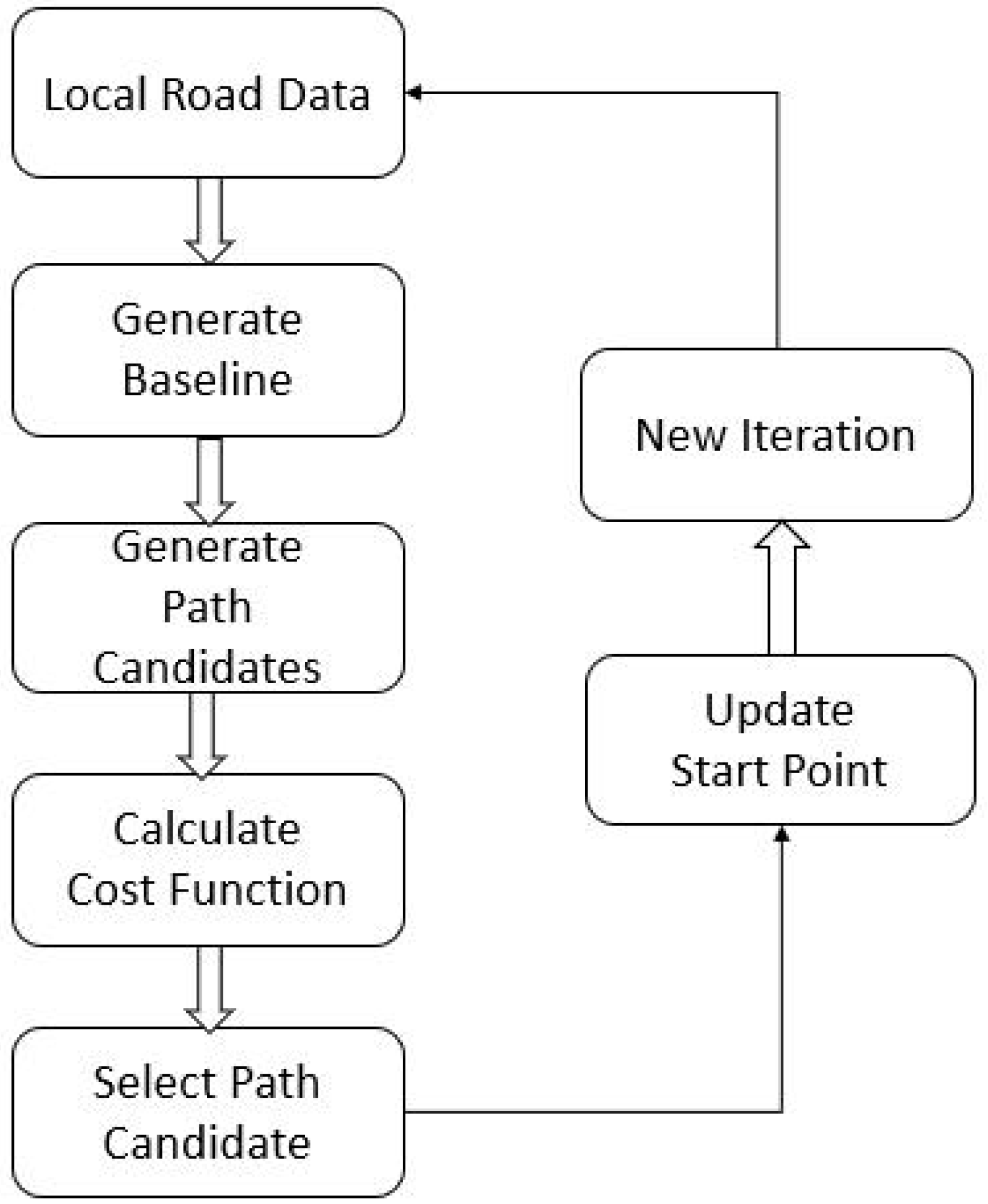
3. Rollover-Free Local Path Planning

This section describes the proposed local path planning method with the incorporation of the vehicle rollover model, also called the rollover-free local path planning method, to build a safe and comfortable path under an appropriate speed and acceleration from an initial location to a destination. The algorithm method aimed to solve a 3D uneven local path planning problem based on a global route and map [29]. With the wide installation of LiDARs and cameras in most autonomous vehicles, we assumed that the 3D occupancy map was generated as the input to the local path planning method. The flowchart of the proposed rollover-free path planning method is given in Figure 3. For a given local road data, i.e., 3D occupancy map with open space and obstacles, we first generated the baseline that describes the curvature of the open space. Based on the current vehicle location and baseline, a group of path candidates were generated, and the optimal path that was collision- and rollover-free and most smooth was selected by evaluating the cost function of all path candidates.

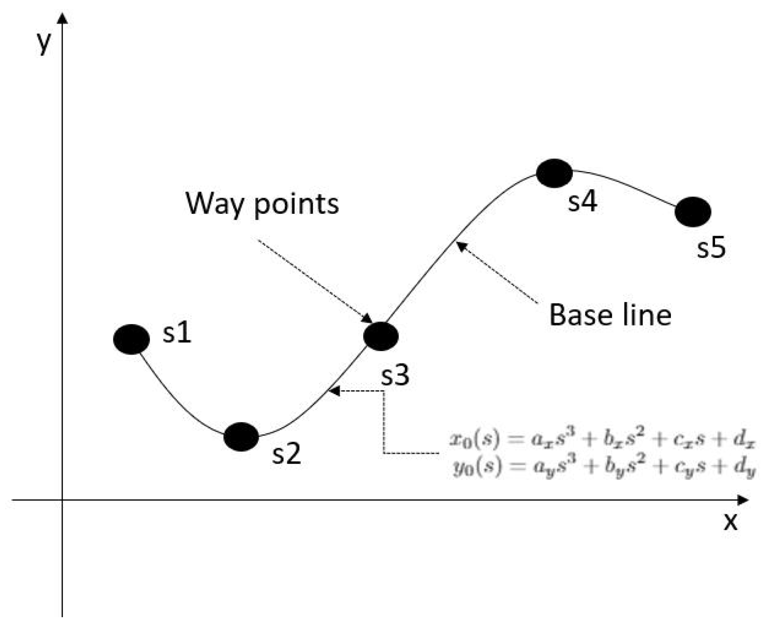
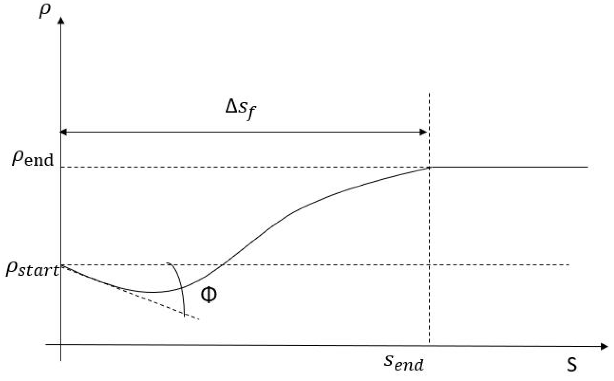
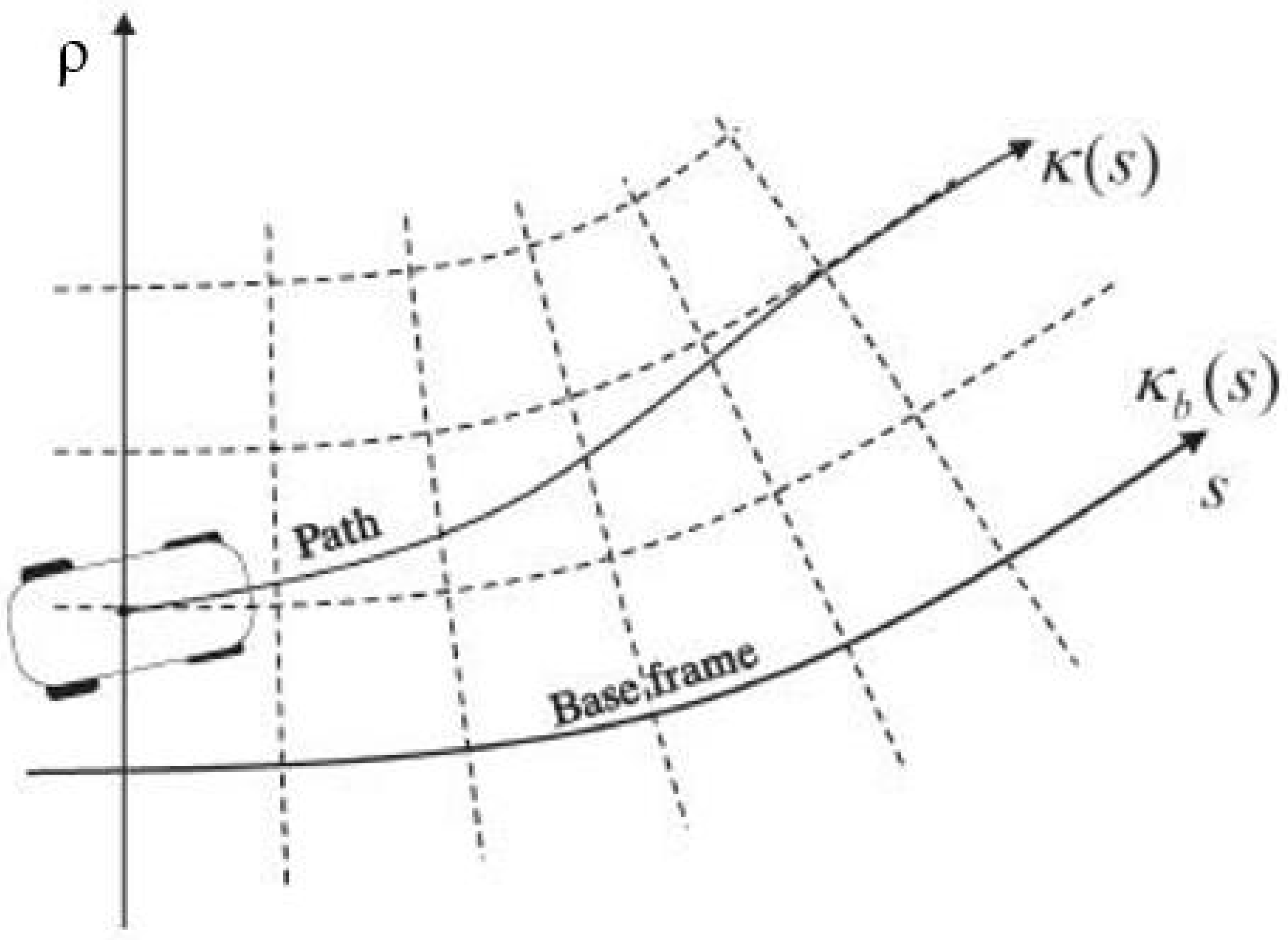
3.1. Off-Road Baseline Construction

Taking the continuity of the first and second derivatives of the curve and computational complexity into consideration, we built a parametric cubic spline to represent the road (i.e., drivable open space) and its baseline. Because the autonomous vehicle usually travels on a route that is not often a regular line, which means the parameter of a typical cubic spline has weak physical meaning, it is also difficult to directly represent the baseline for path planning [30]. The driving path of the autonomous vehicle in this paper is a curve, and the arc length denoted as s is the typical parameter for describing a curve. We used the method of quadrature to calculate the arc length of all segments from the center way-point [31]. The spline can be expressed as Equation (4) [32].

$$\left\{\begin{array}{c}{x}_0\left(s\right)=a_x{s}^3+b_x{s}^2+c_{x}s+d_x\hfill \\ y_0\left(s\right)=a_y{s}^3+b_y{s}^2+c_{y}s+d_y\hfill \end{array}\right.$$

(4)

where ($x_0$, $y_0$) is the Cartesian coordinates of the baseline and $a_x$, $b_x$, $c_x$, $d_x$, and $a_y$, $b_y$, $c_y$, $d_y$ are the coefficients. As shown in Figure 4, the baseline of the bounded road can be divided into many segments by the center way-points. From Equation (4), each road segment can be described by a cubic spline.

We also define a p(s, $\rho$) point system for any point $p_0$ in the plane, which has an offset distance $\rho$ from the baseline. Thus, we can transform the Cartesian coordinates $(x,y)$ into the $s-\rho$ coordinates [33]. With the $s-\rho$ coordinates, we use two additional parameters: the heading ${\theta }_0$ and the curvature $K_b$, to describe the path curve, which can be computed using the first and second derivatives of the cubic spline’s variable s. ${\theta }_0$ can be written by Equation (5),

$${\theta }_0=arctan\frac{d{y}_0}{d{x}_0}$$

(5)

and $K_b$ can be written by Equation (6),

$$K_b=\frac{x_0^{\prime }{y}_0^{″}-x_0^{″}{y}_0^{\prime }}{\sqrt{{(x_0^{\prime }+y_0^{\prime })}^3}}$$

(6)

where $x_0^{\prime }$, $y_0^{\prime }$, $x_0^{″}$, $y_0^{″}$ are the first and second derivatives of $x_0$ and $y_0$ with respect to s.

3.2. Path Candidates’ Generation

As shown in Figure 5, ${\rho }_{start}$ and ${\rho }_{end}$ are the start and end points, respectively, on the baseline in each iteration. Each path candidate has the same travel distance $\Delta s_f$, and we use different offsets $\rho$ from the baseline to generate different path candidates. The following equation is used to describe the relationship between the travel distance s and the offset $\rho$.

$$\rho \left(s\right)=\left\{\begin{array}{c}a{(s-s_{start})}^3+b{(s-s_{start})}^2+c(s-s_{start})+{\rho }_{start}\mathrm{if}s\subset [s_{start},s_{end}]\hfill \\ {\rho }_{end}\mathrm{otherwise}\hfill \end{array}\right.$$

(7)

In Figure 5, the arc length $s_{start}$ and offset ${\rho }_{start}$ at the current location are given by the position on the baseline. The angle $\mathsf{\Phi }$ is defined by the difference between the autonomous vehicle heading angle and the tangent angle of the baseline. In this situation, the boundary condition can be described as Equation (8):

$$\begin{array}{cc}\rho (s=s_{start})={\rho }_{start},\hfill & \rho (s=s_{end})={\rho }_{end}\hfill \\ \frac{d\rho (s=s_{start})}{ds}=tan\Delta {\theta }_{start},\hfill & \frac{d\rho (s=s_{end})}{ds}=0\hfill \end{array}$$

(8)

Thus, {a, b, c, d} are parameters in Equation (7) that can be calculated with the road information condition in Equation (8) when the offset at the endpoint ${\rho }_{end}$ is specified.

As shown in Figure 6, an example of generating the base frame and building path candidates from the center base frame is introduced. This generating process is based on Equations (4)–(8): Firstly, the input data from the autonomous vehicle’s sensors and LiDARs are the local off-road boundary; secondly, a $s-\rho$ coordinates system could be transferred from the Cartesian coordinates road base frame from Equation (4); thirdly, local path candidates in the $s-\rho$ coordinates system are generated by Equations (5)–(8). The generated path candidates’ ranges are related to the shape and range of the local map. Usually, it will be as close as possible to the local road boundary in order to cover a bigger planning space in the local map.

With Equation (7), the path candidates are generated in the s − $\rho$ coordinate system, and they will have to be remapped back to the Cartesian coordinate system so that the vehicle can follow it. As the path candidates are related to the arc length of the baseline, the Cartesian coordinate system value can be represented with s of the baseline [34] as follows in Equations (9)–(11)

$$\frac{dx}{ds}=Acos\theta$$

(9)

$$\frac{dy}{ds}=Asin\theta$$

(10)

$$\frac{d\theta }{ds}=A\kappa$$

(11)

where $\kappa$ is defined as Equation (12),

$$\kappa =\frac{B}{A}\left[K_b+\frac{(1-\rho K_b)\left(\frac{d^2\rho }{d{s}^2}\right)+K_b{\left(\frac{d\rho }{ds}\right)}^2}{A^2}\right]$$

(12)

In Equations (9)–(11), A and B are defined as Equation (13),

$$A=\sqrt{{(\frac{d\rho }{ds})}^2+{(1-\rho K_b)}^2},B=sgn(1-\rho K_b)$$

(13)

where the function of $sgn(1-\rho K_b)$ is −1 when $1-\rho K_b<0$, 1 when $1-\rho K_b>0$, and 0 when $1-\rho K_b=0$. From Equation (9)–(13), we can calculate the Cartesian coordinates (x, y) and the angle $\theta$ for each point of the path candidate.

3.3. Path Selection Algorithm

Once a group of path candidates is generated with the vehicle’s current position and the road baseline, the goal of the path selection algorithm is to select the optimal one that is safe and comfortable to drive, where additional information of an uneven road surface such as obstacles and slopes will be considered. The strategy is to build cost functions in terms of safety and comfortability for each path candidate. In particular, both collision and rollover avoidance were considered in the safety cost function, and both the smoothness and continuity of each path candidate and path unevenness were considered in the comfortability cost function. A two-step cascaded method was used to combine these two cost functions for path selection. A detailed description of these two cost functions is given below.

3.3.1. Cost Function for Driving Safety

To ensure the safety of autonomous driving, the selected path has to be collision- and rollover-free and stay in the local road map. Thus, we consider road range, obstacles, and pits on the road to check the safety of each path candidate.

First of all, each path candidate needs to be checked to determine whether it will run out of the local map. If the path is out of our local map, we set its cost function to the highest value of one.

Secondly, we need to check if a vehicle collision and/or rollover will occur or not for each path candidate. In this paper, we mostly focus on three road conditions in the cost function. At first, each path candidate should be checked for a collision by calculating the entrance and departure angle to the obstacles. If our autonomous vehicle is not able to pass the collision check, there would be no need to build the vehicle rollover model in that situation, thus saving the computational cost. As shown in Figure 7, we used the Cartesian coordinate system to analyze the vehicle moving condition. If there is overlap between the obstacle and the selected path, the obstacle collision will happen, and the highest cost value of one will be assigned to the path candidate.

If there is no obstacle collision, we then check every path candidate’s rollover risk. From Equations (1)–(3), the boundary condition we consider in this paper for a vehicle rollover event is the rollover boundary angle ${\varphi }_0$. If ${\varphi }_0$ is greater than $\varphi$, there would be a high rollover risk, and one has to avoid such a path candidate. To enhance the driving safety, those path candidates that are close to the path leading to a collision or rollover risk are also assigned with the highest risk of one. Mathematically, for the $i^{\mathrm{th}}$ path candidate, we define the cost function for the safety $f_s\left(r_i\right)$ as follows in Equation (14):

$$f_s\left(r_i\right)=\left\{\begin{array}{c}1\mathrm{if}outofmap\hfill \\ 1\mathrm{else}\mathrm{if}obstaclecollision\hfill \\ 1\mathrm{else}\mathrm{if}rollover\hfill \\ 0\mathrm{otherwise}\hfill \end{array}\right.$$

(14)

Suppose that N path candidates are generated at each time step, denoted by $\mathcal{R}=\{r_1,r_2,\cdots ,r_N\}$. For those path candidates that have a safety cost of one, the set of which is denoted by $\mathcal{F}$, we will remove them from further consideration, i.e., ${\mathcal{R}}^{{}^{\prime }}=\mathcal{R}-\mathcal{F}$. For the remaining path candidates that are safe to drive, we further consider their comfortability, which are measured by curve smoothness and continuity, as described next.

3.3.2. Cost Function for Comfortability

For each path candidate that is safe to drive, we further measure its driving comfortability in terms of its smoothness and continuity, as well as its vertical variation. We define the cost function for comfortability as below:

$$f_c\left(r_i\right)=w_s{f}_s\left(r_i\right)+w_v{f}_v\left(r_i\right)$$

(15)

where $f_c\left(r_i\right)$ is the total comfortability cost for the path candidate $r_i$, which consists of two parts: the smoothness cost $f_s\left(r_i\right)$ and the vertical cost $f_v\left(r_i\right)$, weighted by the weights $w_s$ and $w_v$, respectively. In this paper, $w_s=0.5$ and $w_v=0.5$ are used for experimental validation, indicating that each of them contributes equally to the total comfortability cost.

Firstly, if the vehicle runs in a curve with a sharp turn, the passengers easily feels uncomfortable. In this condition, as the smoothness will be directly impacted by the curvature of the path candidates, we will consider the integration of a squared curvature along the length arc s as the smoothness cost for each path candidate, which is given as follows:

$$f_s\left(r_i\right)=\int K_i^2\left(s\right)ds$$

(16)

In this equation, $f_s\left(r_i\right)$ is the smoothness cost value of a path candidate $r_i$ and $K_i\left(s\right)$ is the curvature for the path candidate as a function of the path arc length s.

Secondly, if the vehicle runs on an uneven terrain, the autonomous vehicle will certainly encounter the situation that there are some vertical changes that make passengers uncomfortable. This also happens when it runs through some obstacles and pits that are safe to pass. For a given 3D local map, the vertical change of a path candidate can be measured with its standard deviation $\sigma \left(r_i\right)$ as the cost function:

$$f_v\left(r_i\right)=\sigma \left(r_i\right)$$

(17)

In summary, in our method model, we applied a two-step cascaded mechanism to select the optimal path. In other words, the driving safety was firstly checked, and then, its driving comfortability was further considered. We summarize the pseudocode for path selection with the two cost functions in Algorithm 1: “path candidate selection algorithm for off-road autonomous driving”.

Algorithm 1 Path candidate selection algorithm for off-road autonomous driving.

Require: The set of path candidates: ${\mathcal{R}}_i=\{r_1,r_2,\cdots ,r_N\}$, and 3D local map

1: # Driving Safety Check   2: for$i=1:N$do   3:   if Collision Check is TRUE then   4:     Remove candidate $r_i$ from input set $\mathcal{R}$   5:   else if Rollover Check is TRUE then   6:     Remove candidate $r_i$ from input set $\mathcal{R}$   7:   end if   8: end for   9: # Driving Comfortability Check 10: for$r_k$ in Set $\mathcal{R}$ do 11:   Calculate smoothness cost $f_s\left(r_k\right)$ using Equation (16) 12:   Calculate vertical change cost $f_v\left(r_k\right)$ using Equation (17) 13:   Calculate the total cost: $f_c\left(r_k\right)$ = $w_s{f}_s\left(r_k\right)$ + $w_v{f}_v\left(r_k\right)$ 14: end for 15: Output: A selected path candidate $r^{*}$ that produces the minimum $f_s$: $r^{*}=\underset{r_k\in \mathcal{R}}{arg\; min}{f}_c\left(r_k\right)$.

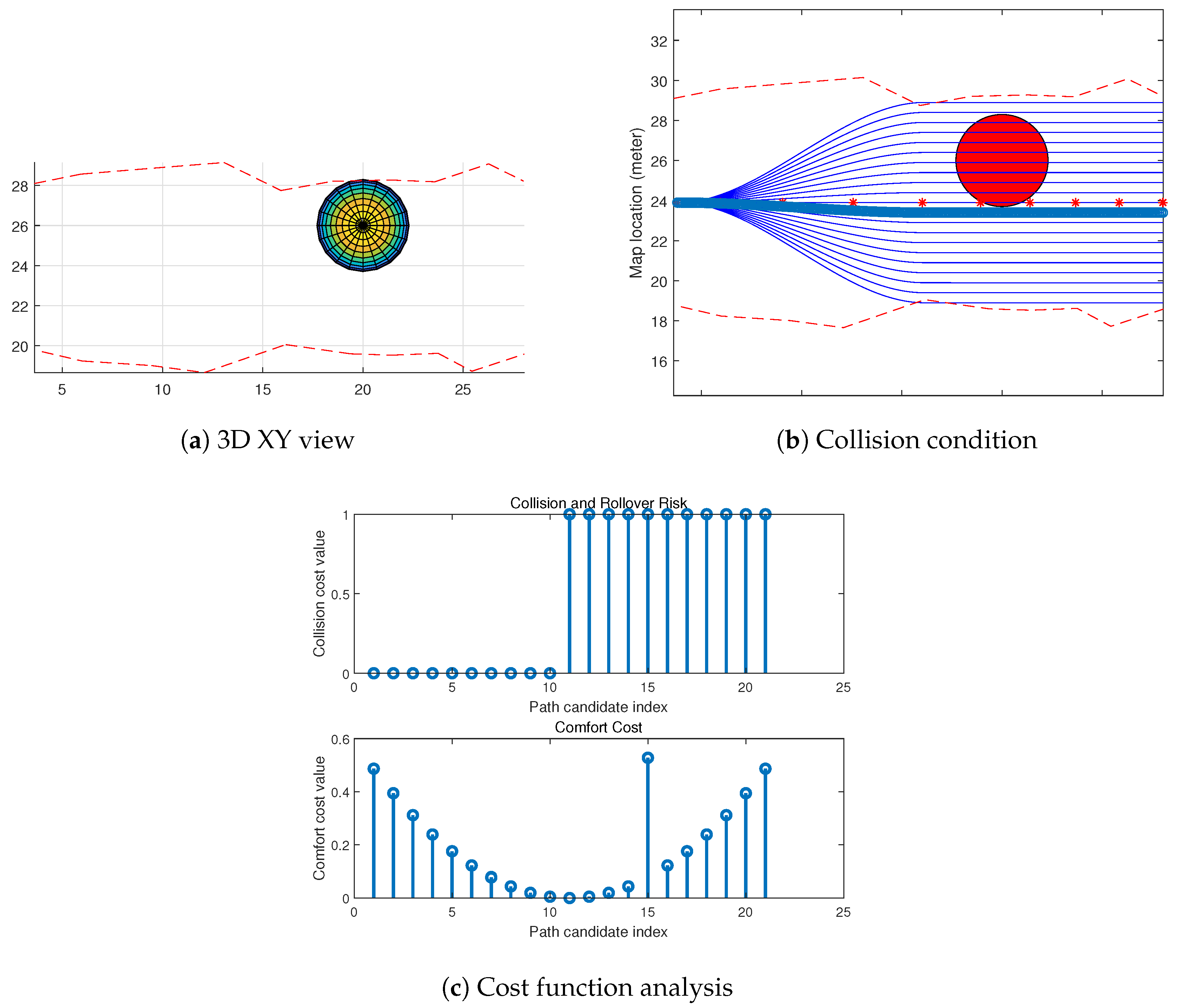
4. Experimental Results and Analysis

Simulations on MATLAB environment are introduced in this section to validate the effectiveness of the proposed collision-free and rollover-free local path planning algorithm in an off-road environment with several uneven obstacles. The cost function analysis is also given under these different road conditions.

For all the simulation figures shown in this section, all path candidates are presented as multiple solid blue lines; the baseline is presented as red stars; and the obstacles are represented as circles. For obstacles that can cause collision risk, the color of the circles is filled with red; for those that can cause rollover risk, the color is set as green; and for those that are safe to pass through, they are shown as transparent circles. The selected path candidate in our simulation is presented as the bold solid blue line. A histogram for discrete sequence data is also given for cost function analysis in each path selection process.

We first show two single static obstacle problems with our path planning algorithm in Figure 8. In Figure 8b, the obstacle filled with red indicates an obstacle that is over the road and causes a collision risk. A path candidate that avoids the risk obstacle is selected based on the minimal comfortable risk result, which is shown in Figure 8c, and the comfortability cost function Equation (16) is related to the candidate length s. In this experiment, the lowest comfortability cost index without collision risk was 10, so we chose the tenth path candidate for decision making. In Figure 9a, the rollover risk is taken into consideration as the autonomous vehicle passes over a hole that is too deep to avoid vehicle rollover risk. The single obstacle filled with green color indicates a static uneven pit on the road. The path selection strategy is similar to the previous collision risk model, and the result is shown in Figure 9b.

In Figure 10, simulations under two types of $A^{*}$ optimal path generation methods [36] are introduced and compared with our proposed method. The optimal path generated by the basic $A^{*}$ algorithm [37] is shown as the solid red line, and the one under the dynamic $A^{*}$ algorithm [38] is shown as the solid black line. The optimal path selected by our proposed method is shown as the bold blue line. We can tell from the simulation results that both basic and dynamic $A^{*}$ methods attempted to find a shortest path between the start point and target by avoiding obstacles. It can be demonstrated that our proposed path planning algorithm had the following advantages, compared to the $A^{*}$ method:

• Firstly, compared to the $A^{*}$ method, the path candidates generated by our method were able to follow the curvature of the baseline using the $s-\rho$ coordinate. This makes the generated paths have less turns on the map, which means it will be more comfortable for passengers in our autonomous vehicles.
• Secondly, the $A^{*}$ method was less efficient at determining the heuristic value when an obstacle was safe to pass, but needed more calculations on the vertical comfortability comparison. However, in our method, we built a good path selection model to find the best path candidate in a local $3D$ map.

As shown in Figure 11a, we imported an $XY$ view to introduce the multiple obstacle passing situation more clearly. The lighter color view indicates that there is an obstacle, i.e., higher than the road surface or $z>0$, and the darker color indicates that there is a pit/hole, i.e., lower than the road surface or $z<0$. In Figure 11b, the proposed path planning algorithm can be also applied to the road with multiple obstacles. There are three obstacles on the road: an obstacle that can cause collision risk colored in red, an obstacle that can cause rollover risk colored in green, and the third obstacle that is safe to pass. In the rollover and collision check part, we can tell by analysis of Figure 11c that only one obstacle is safe to pass, which is the same as the condition we described before. According to the comfortability cost analysis, the optimal path candidate with the minimum comfortability cost is finally selected.

Meanwhile, we conducted simulations by changing the depth of each obstacle and their locations between rollover risk obstacles, collision risk obstacles, and non-rollover risk obstacles. The result showed that in each test, our autonomous vehicle could find the optimal path by our path selection algorithm. The results are shown in Figure 12 and Figure 13.

From Figure 14, we introduce a test while our autonomous vehicle passes through a curve with multiple static obstacles. In Figure 14a, compared to previous straight line simulations, the proposed path planning algorithm method could be applied to a curve with multiple obstacles. In Figure 14b, the collision and rollover cost function and comfort cost function analysis are introduced. From the comfort analysis, it was indicated that the comfort cost when our autonomous vehicle passed a curve had a higher average cost than when it passed a straight line. This higher average result fits the real-world situation and makes our model more realistic. We also introduced a comparison between the $A^{*}$ optimal path generation methods and our autonomous path planning methods, and the result emphasized the first conclusion we made between these two methods. The path candidates generated by our method were able to follow the curvature of the baseline using the $s-\rho$ coordinate. This makes the generated paths have less turns on the map, which means it will be more comfortable for passengers in our autonomous vehicles.

The fourth experiment introduced a test under the road roughness environment. In this situation, we randomly built 100 bumps that were all safe to pass and tested the relationship between the smoothness cost function and the vertical change cost function. The result is shown in Figure 15. We can find from Figure 15b that the best path candidate was Candidate 8. Although Path Candidate 11 had the best performance in the smoothness cost function, it had a higher variance in the vertical change cost function.

The last experiment introduced a test under the road roughness and rollover and collision check environment. In this situation, we randomly built 100 bumps, part of which were safe to pass, while others led to a collision or rollover risk. The result is shown in Figure 16. We can find from Figure 16b that the best path candidate was Candidate 12. Although Path Candidate 10 had the best performance in the comfortability cost function, it could not pass the collision and rollover check. In this paper, we used Equation (15) to calculate the total comfortability cost function, and we used Equation (14) to calculate the collision and rollover risk cost function. The selected path could both avoid collision and rollover risk and have the best comfortability performance among all safe path candidates. This simulation result indicated that our path planning algorithm can be applied in a complex off-road environment.

5. Discussions

In this section, we discuss the computational cost of the proposed rollover-free path planning algorithm and its potential applications in real-world off-road autonomous driving.

Firstly, the computational cost of the proposed path planning algorithm mainly came from two parts: path candidates generation and optimal path selection. To generate a set of N path candidates, each of which consists of K points, the computational cost was $O\left(NK\right)$, and the optimal path selection process had a computational cost of $O\left(N\right)$. The total of the computational cost would be at the scale of $O\left(NK\right)$.

Secondly, the path planning algorithm proposed in this paper relied on the construction of the local 3D occupancy map, which was not the scope of this paper. Currently, most autonomous vehicles are equipped with various kinds of sensors, including LiDARs and stereo cameras, which are able to rebuild a 3D scene of the road. However, it is possible that the shape of some obstacles such as ditches is partially observed, and the missing information such as depths should be estimated. There are two types of methods [39,40]: model-based and learning-based methods to estimate the depth of a ditch. The model-based approach typically assumes that the shape of an obstacle follows a geometrical model, and its unknown parameters can be estimated with partial observations, while the learning-based approach aims to learn a predictive model from raw sensory data and predicts the missing part for a given observation. Once the shape of a ditch is estimated, our vehicle rollover model can be applied to access the risk of vehicle rollover.

Lastly, this paper applies computational simulation techniques to validate the effectiveness of the proposed path planning approaches. Using real-life road data is also of great interest for our future work. However, we also would like to emphasize that computational simulation is preferred for our rollover-free path planning algorithms in off-road autonomous driving, because the safety risk of vehicle rollover is too high in real-life experiments.

6. Conclusions and Future Work

This paper presented a rollover-free path planning method for autonomous driving in an off-road condition with uneven obstacles. First, we built up a rollover model for vehicles running over an obstacle, and then, incorporated it into a local path planning framework, which generated a set of path candidates and selected the ideal path for motion planning. In the path candidate generation, a coordinate transfer from the Cartesian coordinate system to the $s-\rho$ system was applied to describe the information for each path candidate aligned with the baseline. In the path selection, we developed a cost function to select the best candidate in terms of safety, collision, rollover, and smoothness of the path. This function led to the result that the autonomous vehicle could drive safely and tried to follow the curvature of the baseline during driving.

We tested the proposed local path planning using computational experiments with varied road shapes, different sizes and heights of obstacles, and single and multiple obstacles. The results of these experiments showed that our method could identify and choose a safe and smooth path candidate to guide the autonomous vehicle to drive safely and comfortably. Although this paper only considered static obstacles, the proposed method can be easily extended to moving obstacles such as pedestrians and animals, which is a part of our future work. Moreover, in the near future, we also plan to test the performance in a real autonomous vehicle driving in an off-road track.

References

1. Glaser, S.; Vanholme, B.; Mammar, S.; Gruyer, D.; Nouveliere, L. Maneuver-based trajectory planning for highly autonomous vehicles on real road with traffic and driver interaction. IEEE Trans. Intell. Transp. Syst. 2010, 11, 589–606. [Google Scholar] [CrossRef]
2. Zhang, H.; Wang, J. Active steering actuator fault detection for an automatically-steered electric ground vehicle. IEEE Trans. Veh. Technol. 2017, 66, 3685–3702. [Google Scholar] [CrossRef]
3. Hwang, J.; Lee, D.; Huh, K.; Na, H.; Kang, H. Development of a path planning system using mean shift algorithm for driver assistance. Int. J. Autom. Technol. 2011, 12, 119–124. [Google Scholar] [CrossRef]
4. Yang, S.; Cao, Y.; Peng, Z.; Wen, G.; Guo, K. Distributed formation control of nonholonomic autonomous vehicle via RBF neural network. Mech. Syst. Signal Proces. 2017, 87, 81–95. [Google Scholar] [CrossRef]
5. Zhu, M.; Chen, H.; Xiong, G. A model predictive speed tracking control approach for autonomous ground vehicles. Mech. Syst. Signal Proces. 2017, 87, 138–152. [Google Scholar] [CrossRef]
6. Urmson, C.; Anhalt, J.; Bagnell, D.; Baker, C.; Bittner, R.; Clark, M.N.; Dolan, J.; Duggins, D.; Galatali, T.; Geyer, C.; et al. Autonomous driving in urban environments: Boss and the urban challenge. J. Field Robot. 2008, 25, 425–466. [Google Scholar] [CrossRef]
7. Lee, H.-Y.; Shin, H.; Chae, J. Path Planning for Mobile Agents Using a Genetic Algorithm with a Direction Guided Factor. Electronics 2018, 7, 212. [Google Scholar] [CrossRef]
8. Hart, P.E.; Nilsson, N.J.; Raphael, B. RRT-connect: An efficient approach to single-query path planning. In Proceedings of the IEEE International Conference on Robotics and Automation, San Francisco, CA, USA, 24–28 April 2000. [Google Scholar]
9. Barraquand, J.; Langlois, B.; Latombe, J.-C. Numerical potential field techniques for robot path planning. IEEE Trans. Syst. Man Cybern. 1992, 22, 224–241. [Google Scholar] [CrossRef]
10. Tang, W.; Sanville, E.; Henkelman, G. A grid-based Bader analysis algorithm without lattice bias. J. Phys. Condens. Matter 2009, 21, 84–204. [Google Scholar] [CrossRef]
11. Pardalos, P.M.; Prokopyev, O.A.; Busygin, S. Continuous approaches to discrete optimization problems. Nonlinear Optim. Appl. 1996, 313–325. [Google Scholar]
12. Hadsell, R.; Sermanet, P.; Ben, J.; Erkan, A.; Scoffier, M.; Kavukcuoglu, K.; Muller, U.; LeCun, Y. Learning long-range vision for autonomous off-road driving. J. Field Robot. 2009, 26, 120–144. [Google Scholar] [CrossRef] [Green Version]
13. Hussein, A.; Marín-Plaza, P.; Martín, D.; de la Escalera, A.; Armingol, J.M. Autonomous off-road navigation using stereo-vision and laser-rangefinder fusion for outdoor obstacles detection. In Proceedings of the 2016 IEEE Intelligent Vehicles Symposium (IV), Gothenburg, Sweden, 19–22 June 2016; pp. 104–109. [Google Scholar]
14. Raibert, M.; Blankespoor, K.; Nelson, G.; Playter, R. Bigdog, the rough-terrain quadruped robot. IFAC Proc. Vol. 2008, 41, 10822–10825. [Google Scholar] [CrossRef]
15. Semini, C.; Tsagarakis, N.G.; Guglielmino, E.; Focchi, M.; Cannella, F.; Caldwell, D.G. Design of HyQ—A hydraulically and electrically actuated quadruped robot. J. Syst. Control Eng. 2011, 225, 831–849. [Google Scholar] [CrossRef]
16. Wang, L.; Shu, C.; Jin, J.; Zhang, J. A novel traveling wave piezoelectric actuated tracked mobile robot utilizing friction effect. Smart Mater. Struct. 2017, 26, 035003. [Google Scholar] [CrossRef]
17. Zhu, B.; Piao, Q.; Zhao, J.; Guo, L. Integrated chassis control for vehicle rollover prevention with neural network time-to-rollover warning metrics. Adv. Mech. Eng. 2016, 8. [Google Scholar] [CrossRef] [Green Version]
18. Wang, H.; Lyu, W.; Yao, P.; Liang, X.; Liu, C. Three-dimensional path planning for unmanned aerial vehicle based on interfered fluid dynamical system. Chin. J. Aeronaut. 2015, 28, 229–339. [Google Scholar] [CrossRef]
19. Maile, M.; Chen, Q.; Brown, G.; Delgrossi, L. Intersection collision avoidance: From driver alerts to vehicle control. In Proceedings of the 2015 IEEE 81st Vehicular Technology Conference (VTC Spring), Glasgow, UK, 11–14 May 2015; pp. 1–5. [Google Scholar]
20. Cabodi, G.; Camurati, P.; Garbo, A.; Giorelli, M.; Quer, S.; Savarese, F. A Smart Many-Core Implementation of a Motion Planning Framework along a Reference Path for Autonomous Cars. Electronics 2019, 8, 177. [Google Scholar] [CrossRef]
21. National Center for Statistics and Analysis. 2015 Motor Vehicle Crashes: Overview. In Traffic Safety Facts Research Note; National Highway Traffic Safety Administration: Washington, DC, USA, 2016; Volume 2016, pp. 1–9. [Google Scholar]
22. Zhang, D.; Gordon, T.; Gao, Y.; Zong, C.; Lidberg, M. A novel control mediation approach to active rollover prevention. In Proceedings of the 13th International Symposium on Advanced Vehicle Control (AVEC’16), Munich, Germany, 13–16 September 2016; CRC Press: Boca Raton, FL, USA, 2016; p. 203. [Google Scholar]
23. Jiménez, F.; Clavijo, M.; Naranjo, J.E.; Gómez, Ó. Improving the lane reference detection for autonomous road vehicle control. J. Sens. 2016, 2016, 9497524. [Google Scholar] [CrossRef]
24. Chen, B.-C. Warning and Control for Vehicle Rollover Prevention. Ph.D. Thesis, University of Michigan, Ann Arbor, MI, USA, 2001. [Google Scholar]
25. Goodin, C.; Doude, M.; Hudson, C.; Carruth, D. Enabling off-road autonomous navigation-simulation of LIDAR in dense vegetation. Electronics 2018, 7, 154. [Google Scholar] [CrossRef]
26. Hudson, C.R.; Goodin, C.; Doude, M.; Carruth, D.W. Analysis of Dual LIDAR Placement for Off-Road Autonomy Using MAVS. In Proceedings of the IEEE 2018 World Symposium on Digital Intelligence for Systems and Machines (DISA), Kosice, Slovakia, 23–25 August 2018; pp. 137–142. [Google Scholar]
27. Goodin, C.; Carruth, D.; Doude, M.; Hudson, C. Predicting the Influence of Rain on LIDAR in ADAS. Electronics 2018, 8, 89. [Google Scholar] [CrossRef]
28. Goodin, C.; Sharma, S.; Doude, M.; Carruth, D.; Dabbiru, L.; Hudson, C. Training of Neural Networks with Automated Labeling of Simulated Sensor Data; SAE Technical Paper; SAE: Detroit, MI, USA, 2019. [Google Scholar]
29. Choset, H.M.; Hutchinson, S.; Lynch, K.M.; Kantor, G.; Burgard, W.; Kavraki, L.E.; Thrun, S. Principles of Robot Motion: Theory, Algorithms, and Implementation; MIT Press: Cambridge, MA, USA, 2005. [Google Scholar]
30. Ahlberg, J.H.; Nilson, E.N.; Walsh, J.L. The Theory of Splines and Their Applications: Mathematics in Science and Engineering: A Series of Monographs and Textbooks; Elsevier: New York, NY, USA; London, UK, 1967; Volume 38. [Google Scholar]
31. Guenter, B.; Parent, R. Computing the arc length of parametric curves. IEEE Comput. Graph. Appl. 1990, 10, 72–78. [Google Scholar] [CrossRef]
32. Wang, H.; Kearney, J.; Atkinson, K. Arc-length parameterized spline curves for real-time simulation. In Proceedings of the 5th International Conference on Curves and Surfaces, Saint-Malo, France, 27 June–3 July 2002; pp. 387–396. [Google Scholar]
33. Wang, H.; Kearney, J.; Atkinson, K. Robust and efficient computation of the closest point on a spline curve. In Proceedings of the 5th International Conference on Curves and Surfaces, Saint-Malo, France, 27 June–3 July 2002; pp. 397–406. [Google Scholar]
34. Barfoot, T.D.; Clark, C.M. Motion planning for formations of mobile robots. Robot. Auton. Syst. 2004, 46, 365–378. [Google Scholar] [CrossRef]
35. Chu, K.; Lee, M.; Sunwoo, M. Local path planning for off-road autonomous driving with avoidance of static obstacles. IEEE Trans. Intell. Trans. Syst. 2012, 13, 1599–1616. [Google Scholar] [CrossRef]
36. Duchoň, F.; Babinec, A.; Kajan, M.; Beňo, P.; Florek, M.; Fico, T.; Jurišica, L. Path planning with modified a star algorithm for a mobile robot. Procedia Eng. 2014, 96, 59–69. [Google Scholar] [CrossRef]
37. Aslam, J.A.; Pelekhov, E.; Rus, D. The star clustering algorithm for static and dynamic information organization. J. Graph Algorithms Appl. 2004, 8, 95–129. [Google Scholar] [CrossRef]
38. Gil-García, R.; Pons-Porrata, A. Dynamic hierarchical algorithms for document clustering. Pattern Recognit. Lett. 2010, 31, 469–477. [Google Scholar] [CrossRef]
39. Castaño, F.; Beruvides, G.; Haber, R.; Artuñedo, A. Obstacle recognition based on machine learning for on-chip LiDAR sensors in a cyber-physical system. Sensors 2017, 17, 2109. [Google Scholar] [CrossRef] [PubMed]
40. Spagnol, S.; Saitis, C.; Bujacz, M.; Jóhannesson, O.I.; Kalimeri, K.; Moldoveanu, A.; Kristjánsson, A.; Unnthorsson, R. Model-based obstacle sonification for the navigation of visually impaired persons. In Proceedings of the 19th International Conference Digital Audio Effects (DAFx-16), Brno, Czech Republic, 5–9 September 2016; pp. 309–316. [Google Scholar]
Figure 1. Two rollover models: Model “A”, 0DoF, single-unit rigid vehicle model; Model “B”, 1DoF, compliance vehicle model.
Electronics 08 00614 g001
Figure 2. “A”: autonomous car runs into a pit; “B”: autonomous vehicle runs over an obstacle.
Electronics 08 00614 g002
Figure 3. Algorithm flowchart for path planning.
Electronics 08 00614 g003
Figure 4. Baseline and way-points in the Cartesian coordinates: cubic spline baseline function from way-points s 1 s 5 .
Electronics 08 00614 g004
Figure 5. Boundary conditions in the s ρ coordinate system: path candidate from the offset between ρ s t a r t and ρ e n d .
Electronics 08 00614 g005
Figure 6. Example of the generated base frame and path candidates.
Electronics 08 00614 g006
Figure 7. Path candidate and baseline system: the path candidate route follows K ( s ) , which has a close road curvature as the baseline K b ( s ) [35].
Electronics 08 00614 g007
Figure 8. Single obstacle path selection: (a) an XY view on obstacles; the light color indicates z > 0, and the dark color indicates z < 0; (b) path candidate selection under a single obstacle situation; (c) path candidate collision and rollover cost analysis and comfortability cost analysis histogram. All path candidates are presented by multiple solid blue lines; the baseline is presented by red stars; and the obstacles are represented as circles. For obstacles that can cause collision risk, the color of the circles is filled with red; for those that can cause rollover risk, the color is set as green; and for those that are safe to pass through, transparent circles. The selected path candidate in our simulation is presented as the bold solid blue line.
Electronics 08 00614 g008
Figure 9. Single obstacle path selection: (a) path candidate selection under a single pit with rollover risk; (b) path candidate selection under a single pit without rollover risk.
Electronics 08 00614 g009
Figure 10. Comparison between basic A*, dynamic A* and the method in our paper. The obstacles are represented as circles. For obstacles that can cause collision risk, the color of the circles is filled with red; for those that can cause rollover risk, the color is set as green; and for those that are safe to pass through, transparent circles. The method under basic A* is shown by the solid red line; the method under dynamic A* is shown by solid black line; and the method we introduced in our paper is shown by the bold blue line.
Electronics 08 00614 g010
Figure 11. Multiple obstacle path selection: (a) an XY view on obstacles; the light color indicates z > 0; the dark color indicates z < 0; (b) path selection result in a three-obstacle model: the selected path avoids a rollover risk obstacle and a collision risk obstacle and passes over a non-rollover risk obstacle; (c) path candidate collision and rollover cost analysis and comfortability cost analysis histogram.
Electronics 08 00614 g011
Figure 12. Multiple obstacle path selection: (a) an XY view on obstacles; the light color indicates z > 0; the dark color indicates z < 0; (b) path selection result in a three-obstacle model: the selected path avoids two rollover risk obstacles and passes over a non-rollover risk obstacle; (c) path candidate collision and rollover cost analysis and comfortability cost analysis histogram.
Electronics 08 00614 g012
Figure 13. Multiple obstacle path selection: (a) an XY view on obstacles and the boundary; the light color indicates z > 0 ; the dark color indicates z < 0 ; (b) path selection result in a three-obstacle model: the selected path avoids two rollover risk obstacles and passes over a non-rollover risk obstacle; (c) path candidate collision and rollover cost analysis and comfortability cost analysis histogram.
Electronics 08 00614 g013
Figure 14. Multiple obstacle path selection: (a) path selection result in a three-obstacle model: the selected path avoids two rollover risk obstacles and passes over a non-rollover risk obstacle; (b) path candidate collision and rollover cost analysis and comfortability cost analysis histogram; (c) comparison among the dynamic and static A * algorithms and our path planning algorithm.
Electronics 08 00614 g014
Figure 15. Multiple obstacle path selection: (a) a gray map of the XY view on obstacles; the light color indicates z > 0; the dark color indicates z < 0; (b) path selection result under all safe to pass bumps: the selected path finds the best path from the comfortability cost function; (c) path candidate comfortability cost analysis histogram.
Electronics 08 00614 g015
Figure 16. Path planning example: (a) the selected path candidate passes over a non-rollover risk pit; (b) the selected path candidate avoids a rollover risk pit; (c) the path candidate goes back to the baseline from (b) and avoids a collision obstacle.
Electronics 08 00614 g016