A Fast Algorithm for Identifying Density-Based Clustering Structures Using a Constraint Graph

Abstract

OPTICS is a state-of-the-art algorithm for visualizing density-based clustering structures of multi-dimensional datasets. However, OPTICS requires iterative distance computations for all objects and is thus computed in $O\left(n^2\right)$ time, making it unsuitable for massive datasets. In this paper, we propose constrained OPTICS (C-OPTICS) to quickly create density-based clustering structures that are identical to those by OPTICS. C-OPTICS uses a bi-directional graph structure, which we refer to as the constraint graph, to reduce unnecessary distance computations of OPTICS. Thus, C-OPTICS achieves a good running time to create density-based clustering structures. Through experimental evaluations with synthetic and real datasets, C-OPTICS significantly improves the running time in comparison to existing algorithms, such as OPTICS, DeLi-Clu, and Speedy OPTICS (SOPTICS), and guarantees the quality of the density-based clustering structures.

1. Introduction

Clustering is one of the data mining techniques that group data objects based on a similarity [1]. The groups can provide important insights that are used for a broad range of applications [2,3,4,5,6,7,8], such as superpixel segmentation for image clustering [2,3], brain cancer detection [4], wireless sensor networks [5,6], pattern recognition [7,8], and others. We can classify clustering algorithms into centroid, hierarchy, model, graph, density, and grid-based clustering algorithms [9]. Many algorithms address various clustering issues including scalability, noise handling, dealing with multi-dimensional datasets, the ability to discover clusters with arbitrary shapes, and the minimum dependency on domain knowledge for determining certain input parameters [10].

Among clustering algorithms, density-based clustering algorithms can discover arbitrary shaped clusters and noise from datasets. Furthermore, density-based clustering algorithms do not require the number of clusters as an input parameter. Instead, clusters are defined as dense regions separated by sparse regions and are formed by growing due to the inter-connectivity between objects. Density-based spatial clustering of applications with noise (DBSCAN) [11] is a well-known density-based clustering algorithm. To define dense regions which serve as clusters, DBSCAN requires two parameters: $\epsilon$, which represents the radius of the neighborhood of an observed object, and $MinPts$, which is the minimum number of objects in the $\epsilon$-neighborhood of an observed object. Let $P$ be a set of multi-dimensional objects and let the $\epsilon$-neighbors of an object $p_i\in P$ be $N_{\epsilon }\left(p_i\right)$. Here, DBSCAN implements two rules:

• An object $p_i$ is an $\epsilon$-core object if $\left|N_{\epsilon }\left(p_i\right)\right|\ge MinPts$;
• If $p_i$ is an $\epsilon$-core object, all objects in $N_{\epsilon }\left(p_i\right)$ should appear in the same cluster as $p_i$.

The process of DBSCAN is simple. Firstly, an arbitrary $\epsilon$-core object $p_i$ is added to an empty cluster. Secondly, a cluster grows as follows: for every $\epsilon$-core object $p_i$ in the cluster, all objects of $N_{\epsilon }\left(p_i\right)$ are added to the cluster. This process is then repeated until the size of a cluster no longer increases. However, DBSCAN cannot easily select appropriate input parameters to form suitable clusters because the input parameters depend on prior knowledge, such as the distribution of objects and the ranges of datasets. Moreover, DBSCAN cannot find clusters of differing densities. Figure 1 demonstrates this limitation of DBSCAN in a two-dimensional dataset $P$ when $MinPts=3$. If $\epsilon =0.955$, $p_2$ is an $\epsilon$-core object and forms a cluster, which contains $p_1$, $p_2$, $p_3$, and $p_4$ because $\left|N_{\epsilon }\left(p_2\right)\right|\ge MinPts$ is satisfied. However, $p_9$ and $p_{13}$ are noise objects. Here, a noise object is an object that is not included in any cluster. In other words, a set of objects that cannot reach $\epsilon$-core objects in the clusters are defined as noise objects. On the other hand, if $\epsilon =1.031$, $p_{13}$ becomes an $\epsilon$-core object and forms a cluster, which contains $p_{11}, p_{13}$, and $p_{12}$. However, $p_9$ is still a noise object. As shown in the example in Figure 1, input parameter selection in DBSCAN is problematic.

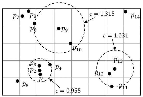
Figure 1. Two-dimensional clustering example demonstrating problems of density-based spatial clustering of applications with noise (DBSCAN) for the selection of $\epsilon$ ($MinPts=3$).

To address this disadvantage of DBSCAN, a method for ordering points to identify the clustering structure, called OPTICS [12], was proposed. Like DBSCAN, OPTICS requires two input parameters, $\epsilon$, and $MinPts$, and finds clusters of differing densities by creating a reachability plot. Here, the reachability plot represents an ordering of a dataset with respect to the density-based clustering structure. To create the reachability plot, OPTICS forms a linear order of objects where objects that are spatially closest become neighbors [13]. Figure 2 shows the reachability plot for a dataset $P$, when $\epsilon =\sqrt{2}$ and $MinPts=3$. The horizontal axis of the reachability plot enumerates the objects in a linear order, while vertical bars display reachability distance (see Definition 2), which is the minimum distance for an object to be included in a cluster. The reachability distances for some objects (e.g., $p_1$, $p_6$, $p_{11}$, and $p_{14}$) are infinite. In this case, an infinite reachability distance results when the distance to each object is undefined because the distance value is greater than given $\epsilon$. OPTICS does not provide clustering results explicitly, but the reachability plot shows the clusters for $\epsilon$. For example, when $\epsilon =0.5$, a first cluster $C_1$ containing $p_1$, $p_2$, and $p_3$ is found. When $\epsilon =0.943$, second cluster $C_2$, which contains $p_6$, $p_7$, and $p_8$ is found. As $\epsilon$ grows larger, clusters $C_1$ and $C_2$ continue to expand, and a third cluster $C_3$ containing $p_{11}$, $p_{12}$, and $p_{13}$ is found.

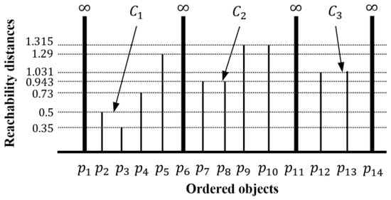
Figure 2. A reachability plot of an example dataset ($\epsilon =\sqrt{2}$ and $MinPts=3$).

As demonstrated in Figure 2, OPTICS addresses the limitations of input parameter selection for DBSCAN. However, OPTICS requires distance computations for all pairs of objects to create a reachability plot. In other words, OPTICS first computes an $\epsilon$-neighborhood for each object to identify $\epsilon$-core objects, and then, computes reachability distances at which $\epsilon$-core objects are reached from all other objects. Thus, OPTICS is computed in $O\left(n^2\right)$ time, where $n$ is the number of objects in a dataset [14]. Therefore, OPTICS is unsuitable for massive datasets. Prior studies have proposed many algorithms to address the running time of OPTICS, such as DeLi-Clu [15] and SOPTICS [16]. These algorithms improve the running time of OPTICS, but have their own limitations such as dependence on the number of dimensions, and deformation of the reachability plot.

This paper focuses on improving OPTICS by addressing its quadratic time complexity problem. To do this, we propose a fast algorithm, called constrained OPTICS (simply, C-OPTICS). C-OPTICS uses a novel bi-directional graph structure, called the constraint graph, which consists of the vertices corresponding to each cell that partitions a given dataset. In the constraint graph, the vertices are linked by means of edges when the distance between vertices is less than an $\epsilon$. The constraints are assigned as the weight of each edge. The main feature of C-OPTICS is that it only computes the reachability distances of the objects that satisfy the constraints, which results in a reduction of unnecessary distance computations when creating a reachability plot. We evaluated the performance of C-OPTICS through experiments with the OPTICS, DeLi-Clu, and SOPTICS algorithms. The experimental results show that C-OPTICS significantly reduces the running time compared with OPTICS, DeLi-Clu, and SOPTICS algorithms and guarantees the reachability plot identical to those by of OPTICS.

The rest of the paper is organized as follows: Section 2 provides an overview of OPTICS, including its limitations, and describes related studies that have been performed to improve OPTICS. Section 3 defines the concepts of C-OPTICS and describes the algorithm. Section 4 presents an evaluation of C-OPTICS based on the results of experiments with synthetic and real datasets. Section 5 summarizes and concludes the paper.

2. Related Work

This section focuses on OPTICS and related algorithms proposed to address the quadratic time complexity problem of OPTICS. Section 2.1 presents the concepts of OPTICS and discusses unnecessary distance computations in OPTICS. Section 2.2 describes the existing algorithms proposed to improve the running time of OPTICS. Details of all the symbols used in this paper are defined in Table 1.

Table 1. The notations.

Symbols	Definitions
$P$	A set of $N$ objects for clustering
$N$	The cardinality of $P$
$p_i$	An i-th object (or data point) in $P$ ($1\le i\le N$)
$UC$	Unit cell that partitions the dataset (Definition 3)
$d$	The number of dimensions of $P$
$MBR$	The minimum bounding rectangle in $UC$
$v$	A vertex in the constraint graph
$C$	The cluster of $P$
$\epsilon$	Epsilon represents the radius of neighborhood of an object $p_i$
$MRD$	The maximum reachable ranges of a vertex by $\epsilon$ (Definition 4)
$N_{\epsilon }\left(p_i\right)$	The $\epsilon$-neighborhood of an object $p_i$
$MinPts$	Minimum number of objects in the $\epsilon$-neighborhood of an object $p_i$
$cdis{t}_{\epsilon , MinPts}\left(p_i\right)$	The core distance of $p_i$ (Definition 1)
$rdis{t}_{\epsilon , MinPts}\left(p_i, p_j\right)$	The reachability distance of an object $p_i$ w.r.t. an $\epsilon$-core object $p_j$ (Definition 2)
$dist\left(p_i, p_j\right)$	The distance between $p_i$ and $p_j$
$vdist\left(v_i, v_j\right)$	The distance between two vertices $v_i$ and $v_j$
$RV$	The set of adjacent vertices for a vertex $v$
$vstate$	The state of a vertex $v$ (Definition 6)
$LC\left(v_i, v_j\right)$	The linkage constraint from $v_i$ to $v_j$ (Definition 5)

2.1. OPTICS

The well-known hierarchical density-based algorithm OPTICS visualizes the density-based clustering structure. Section 2.1.1 reviews the definitions of the naïve algorithm used to compute a reachability plot. Section 2.1.2 demonstrates the quadratic time complexity of the naïve algorithm and its unnecessary distance computations.

2.1.1. Definitions

Let $P$ be a set of $n$ objects in the $d$-dimensional space ${ℝ}^d$. Here, the Euclidean distance between two objects $p_i$ and $p_j$ is denoted by $dist\left(p_i, p_j\right)$. OPTICS creates a reachability plot based on the concepts defined below.

Definition 1

(Core distance of an object$p$) [12]. Let $N_{\epsilon }\left(p\right)$ be the $\epsilon$-neighborhood and let $MinPts$-$dist\left(p\right)$ be the distance between $p$ and $MinPts$-th nearest neighbor. The core distance of $p$, $cdis{t}_{\epsilon , MinPts}\left(p\right)$, is then defined using Equation (1):

$$cdis{t}_{\epsilon , MinPts}\left(p\right)=\{\begin{array}{r}UNDEFINED, \left|N_{\epsilon }\left(p\right)\right|<MinPts\\ MinPts-dist\left(p\right), otherwise\end{array}.$$

(1)

Note that $cdis{t}_{\epsilon , MinPts}\left(p\right)$ is the minimum $\epsilon$ at which $p$ qualifies as an $\epsilon$-core object for DBSCAN. For example, when $\epsilon =\sqrt{2}$ and $MinPts=3$ for the sample dataset $P$ in Figure 1, $cdis{t}_{\sqrt{2}, 3}\left(p_9\right)=1.315$, which is the distance between $p_9$ and the $MinPts$-th nearest neighbor $p_6$.

Definition 2

(Reachability distance object$p$with respect to object$o$) [12]. Let $p$ and $o$ be objects from dataset $P$; the reachability distance of $p$ with respect to $o$, $rdis{t}_{\epsilon , MinPts}\left(p, o\right)$, is defined as Equation (2):

$$rdis{t}_{\epsilon , MinPts}\left(p, o\right)=\{\begin{array}{c}UNDEFINED, \left|N_{\epsilon }\left(o\right)\right|<MinPts\\ max\left(cdis{t}_{\epsilon , MinPts}\left(o\right), dist\left(o, p\right)\right), otherwise\end{array}.$$

(2)

Intuitively, when $o$ is an $\epsilon$-core object, the reachability distance of $p$ with respect to $o$ is the minimum distance such that $p$ is directly density-reachable from $o$. Thus, the minimum reachability distance of each object $p\in P$ means the minimum distance that can be contained in a cluster. To create a reachability plot, a linear order of objects is formed by selecting a next object $p$ that has the closest reachability distance to an observed object $o$. Here, a linear order of objects represents the order of interconnection between objects by densities in the dataset. Accordingly, the reachability plot shows the reachability distance for each object in the order the object was processed.

2.1.2. Computation

OPTICS first finds all $\epsilon$-core objects in the dataset at $O\left(n^2\right)$ time and then computes the minimum reachability distance for all objects at $O\left(n^2\right)$ time to create a reachability plot. This is still the best time complexity known. Alternatively, $\epsilon$-core objects can be found quickly using spatial indexing structures, such as an R*-tree [17], that optimize range queries to obtain $\epsilon$-neighborhoods. However, the reachability plot is still created at $O\left(n^2\right)$ time because computing the reachability distances of all objects to form a linear order of objects is not optimized by the spatial indexing structure. In other words, OPTICS has quadratic time complexity because each object computes reachability distances for all $\epsilon$-core objects in the dataset. However, only the minimum reachability distance of each object is displayed in the reachability plot (see Figure 2). That is, all reachability distance computations, except for identifying the reachability distance displayed in the reachability plot, are unnecessary.

Figure 3 shows an example of unnecessary reachability distances for sample dataset $D$ when $\epsilon =\sqrt{2}$ and $MinPts=3$. First, the distance between $p_1$ and all sample objects $p_i\in N_{\epsilon }\left(p_1\right)$ is computed to determine if $p_1$ is a core object. Next, the distance between $p_1$ and the $MinPts$-th nearest neighbor is computed to obtain the core distance of $p_1$ according to Definition 1. Subsequently, the reachability distances for all objects contained in $N_{\epsilon }\left(p_1\right)$ are computed according to Definition 2 as shown in Figure 3a. That is, the reachability distances between $p_1$ and $p_2$, $p_3$, $p_4$, $p_5$ are computed. This process is repeated for all sample objects as shown in Figure 3b. However, as shown in Figure 3c, not all reachability distances are required to create a reachability plot. For example, $p_5$ is reachable from both $p_1$ and $p_2$; however, a reachability distance from $p_1$ is 1.29 and from $p_2$ is 1.37. Considering that only the minimum reachability distance of each object is displayed in the reachability plot, the reachability distance computation from $p_5$ to $p_2$ is unnecessary because it does not contribute to creating a reachability plot.

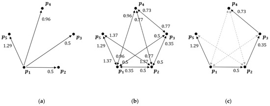
Figure 3. Visualization of the reachability distances for sample dataset $D$: (a) all reachability distances for $p_1$; (b) all reachability distances between sample objects; (c) unnecessary distance computations between sample objects.

2.2. Existing Work

This subsection describes the algorithms proposed to address the quadratic time complexity of OPTICS. Researchers have proposed new indexing structures and approximate reachability plot to reduce the number of core distance and reachability distance computations. In addition, some researchers have proposed algorithms to visualize a new hierarchical density-based clustering structure. We can classify these algorithms roughly into the following three categories: equivalent algorithms with results identical to those of OPTICS, approximate algorithms, and other hierarchical density-based algorithms.

Among the equivalent algorithms, DeLi-Clu [15] optimized range queries to compute the core distance and reachability distance of each object in a dataset using a spatial indexing structure, in this case, the variance of R*-tree. In particular, the proposed self-join R*-tree query significantly reduces the total number of distance computations. Furthermore, DeLi-Clu discards a parameter $\epsilon$, as the join process will automatically stop when all objects are connected, without computing all pair-wise distances. However, as the dimension of the dataset increases, the limitations of R*-tree arise in the form of overlapping distance computations, which significantly degrades the performance of DeLi-Clu. The extended DBSCAN and OPTICS algorithms are proposed by Brecheisen et al. [18]. These two algorithms improved the performances of DBSCAN and OPTICS by applying a multi-step query processing paradigm. Specifically, the core distance and reachability distance were quickly computed by replacing range queries with $MinPts$-th nearest neighbor queries. In addition, complicated distance computations were performed only at essential steps to create a reachability plot to reduce waste computations. However, the running time of the extended DBSCAN and OPTICS in [18] is not suitable for massive datasets. Other approaches which use exact algorithms are those based on a graphics processing unit (GPU), or multi-core based distributed algorithms. One study [13] introduced an extensible parallel OPTICS algorithm on a 40-core shared memory machine. The similarities between OPTICS and Prim’s minimum spanning tree algorithm were used to extract clusters in parallel from the shared memory. Other work [19] introduced G-OPTICS, which improves the scalability of OPTICS using a GPU. G-OPTICS significantly reduces the running time of OPTICS by processing the iterative computations required to form a reachability plot in parallel through the GPU and shared memory.

Approximate algorithms simplify and reduce the complex distance computations of OPTICS. An algorithm was proposed to compress the dataset with data bubbles containing only key information [20]. The number of distance computations is determined via the data compression ratio, allowing the scalability to be improved. However, if the data compression ratio exceeds a certain level, the reachability plot identical to those by of OPTICS cannot be guaranteed. The higher the data compression ratio, the larger the number of objects abstracted into only a representative object. GridOPTICS, which transforms the dataset into a grid structure to create a reachability plot, was proposed [21]. GridOPTICS initially creates a grid structure for a given dataset, after which it forms a reachability plot for the grids. It then assigns objects in the dataset to the formed reachability plot. However, clustering quality is not guaranteed given that the form of the reachability plot depends on the size of the grids. Another method is SOPTICS [16], which applies random projection to improve the running time of OPTICS. After partitioning a dataset into subsets while performing random projection via a pre-defined criterion, it quickly creates a reachability plot using a new density estimation metric based on average distance computations through data sampling. However, SOPTICS includes many deformations in the reachability plot due to the random projection maps objects into the lower dimensions.

Other hierarchical density-based clustering algorithms have been continuously studied. A runt-pruning algorithm that analyzes the minimum spanning tree of the sampled dataset and then uses nearest neighbor-based density estimation to define the density levels of each object to create a cluster tree was proposed in [22]. Based on a runt test for multi-modality [23], the runt-pruning algorithm creates a cluster tree by repeating the task of partitioning a dense cluster into two connected components. HDBSCAN, which constructs a graph structure with a mutual reachability distance between two objects, was also proposed in [24]. It discovers a minimum spanning tree and then forms a hierarchical clustering structure. In addition to hierarchical clustering, an algorithm for producing flat partitioning from the hierarchical solution was introduced in [25].

3. Constrained OPTICS (C-OPTICS)

3.1. Overview

We now explain the proposed algorithm, called C-OPTICS. The goal of the C-OPTICS is to reduce the total number of distance computations required to create a reachability plot because they affect the running time of OPTICS, as explained in Section 2.1.2. To achieve this goal, C-OPTICS proceeds in three steps: (a) partitioning step, (b) graph construction step, and (c) plotting step. For the convenience of the explanation, Figure 4 shows the process of the C-OPTICS for the two-dimensional dataset $P$ in Figure 1. In the partitioning step, we partition $P$ into identical cells. Figure 4a shows the result of partitioning, where empty cells are discarded. In the graph construction step, as shown in Figure 4b, we construct a constraint graph that consists of vertices corresponding to the cells obtained in the partitioning step and edges linking vertices by constraints. In the plotting step, we compute the reachability distance of each object while traversing the constraint graph. Figure 4c shows the reachability distance and linear order of each object.

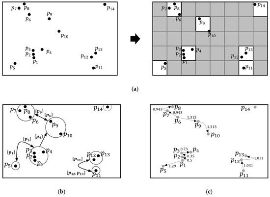
Figure 4. The overall process of the C-OPTICS for the two-dimensional dataset $P$: (a) partitioning step, (b) graph construction step, and (c) plotting step.

C-OPTICS can obtain $\epsilon$-neighbors by finding adjacent cells for an arbitrary object. Thus, C-OPTICS can reduce the number of distance computations to find $\epsilon$-core objects. Besides, C-OPTICS only computes the reachability distances of the objects that satisfy the constraints in the constraint graph. Consequently, C-OPTICS reduce the total number of distance computations required to create a reachability plot. We explain in detail the partitioning step in Section 3.2, the graph construction step in Section 3.3, and the plotting step in Section 3.4.

3.2. Partitioning Step

This subsection describes the data partitioning step for C-OPTICS. We partition a given dataset into cells of identical size with a diagonal length $\epsilon$. Definition 3 explains the unit cell of the partitioning step.

Definition 3

(Unit cell,$UC$). We define$UC$as a$d$-dimensional hypercube with a diagonal length$\epsilon$and straight sides, all of equal length.$UC$is a square with a diagonal length$\epsilon$in two dimensions, and in three dimensions$UC$is a cube with a diagonal length$\epsilon$.

Here, all $UC$s have two main features. First, each $UC$ has a unique identifier that is used as the location information in the dataset. We use the coordinates values of a $UC$ to obtain a unique identifier. Here, the coordinates value of a $UC$ represents a sequence of $UC$ for each dimension in the dataset. Thus, combining the coordinates values of $UC$ for all dimensions enables us to obtain the location information from a unique identifier. The location information can quickly find adjacent $UC$s within a radius $\epsilon$ for an arbitrary $UC$. Through partitioning step, we can reduce the number of distance computations in finding $\epsilon$-neighbors of each object because the number of objects in each cell within a radius $\epsilon$ is smaller than in the entire dataset. We can further simplify the process of constructing a constraint graph in a later step. Second, each $UC$ has a $d$-dimensional minimum bounding rectangle ($MBR$) that encloses the contained objects. We use $MBR$s to compute the distance between $UC$s to find adjacent $UC$s. We obtain all coordinates of $MBR$ based on the maximum and minimum values of each dimension for the contained objects. If the $UC$ contains only one object, the object becomes an $MBR$.

Example 1.

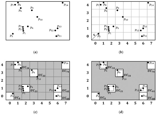
Figure 5 shows an example of the partitioning step for the sample dataset$P$when$\epsilon =\sqrt{2}$. Figure 5a shows each object$p_i\in P$in a two-dimensional universe.Figure 5b shows the partitioning of$P$into$UC$s, where each UC has the same diagonal length.Figure 5c shows empty and non-empty$UC$s. Note that we do not consider empty$UC$s. Further, we obtain the unique identifier of each$UC$as follows. To compute the unique identifier of$U{C}_{21}$, we first obtain the coordinate values of$U{C}_{21}$in each dimension. As shown inFigure 5c, the coordinate values of$U{C}_{21}$are (2,1) in the first and second dimensions, respectively. Considering that a unique identifier of$U{C}_{21}$is obtained by the combination of the coordinate values, the unique identifier of$U{C}_{21}$is 21. The result of partitioning is shown inFigure 5d, where$P$is partitioned into seven$UC$s, with each$UC$having a$MBR$.

Figure 5. Partitioning into $UC$s of sample dataset $P$ ($\epsilon =\sqrt{2}$): (a) the sample dataset $P$, (b) $UC$s that partition $P$, (c) non-empty $UC$s (white area) and their unique identifiers, and (d) the result of the partitioning step.

3.3. Graph Construction Step

In the graph construction step, we construct a constraint graph with the $UC$s obtained in the data partitioning step. Through constructing a constraint graph, we can reduce the number of distance computations to obtain the minimum reachability distance for each object. For this, we first use the $UC$s obtained in the data partitioning step as the vertices of the constraint graph. Here, a unique identifier of each $UC$ is used as a unique identifier of each vertex. Thus, we can quickly find adjacent vertices because we preserve the location information of $UC$ for each vertex. Additionally, we also preserve the $MBR$ of each $UC$. Then, we connect the vertices to define the edges. Here, we connect the vertices according to two properties: (i) the two vertices must be adjacent to each other within a radius $\epsilon$, and (ii) an edge between two vertices must have constraints. Considering that we can quickly find the $\epsilon$-neighborhood of each object in the dataset by the first property, we can obtain the objects that are within a radius $\epsilon$. Thus, there is no need to compute distances with all objects. We first explain the maximum reachability distance, which is defined as Definition 4.

Definition 4

(Maximum reachability distance,$MRD$). We define$MRD$as the range of a radius$\epsilon$at which a vertex can reach. Here, the unique identifier of a vertex is the combination of coordinate values. Thus, in$d$-dimension,$MRD$represents$\pm \sqrt{d}$range for a coordinate value of each dimension because a radius$\epsilon$is$\sqrt{d}$times the length of a straight side of$UC$that corresponds to the vertex.

Figure 6 shows an example of the $MRD$ for a vertex, $v_{33}$, in two-dimensional space. We can decompose the unique identifier of $v_{33}$ into two coordinates values, which are (3, 3). Considering that the MRD of a vertex in the two-dimensional dataset represents a range of +2 and −2 in coordinate values of each dimension, according to Definition 4, the reachable range of each dimension is 1 to 5 in the first dimension and 1 to 5 in the second dimension. As a result, the $MRD$ of $v_{33}$ is equal to the gray area shown in Figure 6. Through the calculation of MRD, we can find adjacent vertices within the same range and thus, avoid unnecessary calculations of distances between all vertices. In Figure 6, adjacent vertices $v_{12}$ and $v_{53}$ are in the $MRD$ of $v_{33}$.

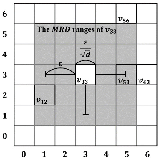
Figure 6. An example of maximum reachability distance ($MRD$) in two-dimensional space.

Additionally, we use the $MBR$ of each vertex to compute the distance between two vertices. We can obtain the adjacent vertices more accurately by computing the distance between the two vertices. Here, adjacent vertices obtained from $MRD$ of an arbitrary vertex may not actually be vertices within a radius $\epsilon$ because the range of $MRD$ and the range of $\epsilon$ do not precisely match. Thus, we compute the minimum distance between the $MBR$s of two vertices to find adjacent vertices within the radius $\epsilon$. Equation (3) represents the distance between two vertices.

$$vdist\left(v_i, v_j\right)=\min \left(dist\left(v_i.MBR, v_j.MBR\right)\right),$$

(3)

where $vdist\left(v_i, v_j\right)$ is the distance between $v_i$ and $v_j$. $v_i.MBR$ is the $MBR$ of a unit cell $U{C}_i$ corresponding to $v_i$. Here, if $vdist\left(v_i, v_j\right)\le \epsilon$, $v_j$ is the adjacent vertex of $v_i$ and vice versa.

Next, we define the constraints to link vertices that satisfy the second property. Recall from Section 1 that the constraint graph only links vertices when the distance between vertices is less than an ε. These pairs of vertices become edges, and the constraints are assigned as weights for each edge. Here, the constraint is defined as a subset of $\epsilon$-core objects that can compute the minimum reachability distances of objects in different vertices. In the plotting step, we only compute the reachability distances of the objects that satisfy the constraints and thus, reduce unnecessary distance computations. Here, a constraint is satisfied if the observed object belongs to a subset of $\epsilon$-core objects as designated by the constraint. We first explain the linkage constraints defined as Definition 5 to obtain the $\epsilon$-core objects corresponding to the constraints.

Definition 5.

(Linkage constraint,$LC\left(v_i, v_j\right)$) For two vertices$v_i$and$v_j$, let an$\epsilon$-core object in$v_i$be$p_{core}$and let the$MBR$of a vertex$v_j$be$v_j.MBR$. We define the linkage constraint from$v_i$to$v_j$as a subset of$\epsilon$-core objects in$v_i$. Here, when$p_1$is an$\epsilon$-core objectclosest to the$v_j.MBR$and$q$is the coordinates of$v_j.MBR$farthest from$p_1$, the$\epsilon$-core objectsshould be closer to$q$than they are to$p_1$.

We link two vertices when the linkage constraint between the vertices is defined according to Definition 5. Thus, we can reduce unnecessary distance computations by pruning the adjacent vertices obtained in the first property again. Furthermore, the linkage constraints guarantee the quality of the reachability plot while reducing the number of distance computations. We prove this in Lemma 1.

Lemma 1.

Let the linkage constraint from$v_i$to$v_j$be$LC\left(v_i, v_j\right)$for$v_i,v_j\in V$in the constraint graph$G\left(V, E\right)$. If$LC\left(v_i, v_j\right)\ne \varnothing$, the minimum reachability distances for all objects contained in$v_j$are determined by the$LC\left(v_i, v_j\right)\times v_j$pair and the core distance. In other words, the reachability distances of all objects in$v_j$are determined by$\epsilon$-core objects in$LC\left(v_i, v_j\right)$.

Proof. 

For a given dataset $P$, let $v_i=\left\{p_1, p_2\right\}$, $p_t\in v_j$ and let the linkage constraint $LC\left(v_i, v_j\right)=\left\{p_1\right\}$ from $v_i$ to $v_j$. In this case, the reachability distance of an object $p_t$ is determined by $p_1$ when $cdis{t}_{\epsilon , MinPts}\left(p_1\right)\le dist\left(p_1, p_t\right)$. Conversely, $p_2$ cannot determine the reachability distance of $p_t$ because $cdis{t}_{\epsilon , MinPts}\left(p_1\right)<dist\left(p_2, p_t\right)$ holds in all cases even when $dist\left(p_1, p_t\right)<cdis{t}_{\epsilon , MinPts}\left(p_1\right)$. Therefore, Lemma 1 is obviously true. □

Additionally, we define the state of a vertex. We can find $\epsilon$-core objects in the dataset without computing the distance between the objects through the states of vertices. We define the state of a vertex based on the rules of DBSCAN, and from the $UC$s obtained in the data partitioning step. As described in Section 1, if the number of objects contained in the $\epsilon$-neighborhood for an arbitrary object is greater than or equal to $MinPts$, then the object is an $\epsilon$-core object. Here, because the diagonal length of $UC$ is $\epsilon$, the objects must be $\epsilon$-core objects when the number of objects contained in $UC$ is greater than or equal to $MinPts$. Accordingly, we define three states for each vertex: $stable$, $unstable$, and $noise$. More precisely, the state of a vertex is defined as follows:

Definition 6.

(The state of a vertex,$vstate$) Let a set of adjacent vertices contained in$MRD$of$v_i$be$R{V}_i$and an adjacent vertex be$r{v}_k\in R{V}_i$. The state of$v_i$, which can determine whether to compute the distance of contained objects, satisfies the following conditions:

1. 

Let$\left|v_i\right|$be the number of data points contained in$v_i$. If$MinPts\le \left|v_i\right|$,$v_i.vstate$is$stable$;

2. 

If condition 1 is not satisfied and$MinPts\le \left|v_i\right|+\left|r{v}_k\right|$,$v_i.vstate$is$unstable$;

3. 

If both conditions 1 and 2 are not satisfied,$v_i.vstate$is$noise$.

Again, we denote that objects contained in the same vertex must be $\epsilon$-neighbor for each other. Thus, when the $vstate$ of a vertex $v_i$ is $stable$, all objects contained in $v_i$ are $\epsilon$-core objects, because the $\left|N_{\epsilon }\left(p_t\right)\right|$ of all objects $p_t\in v_i$ is always greater than or equal to $MinPts$. Conversely, if the $vstate$ of $v_i$ is $noise$, all objects contained in $v_i$ are noise objects and are not considered anymore.

Example 2.

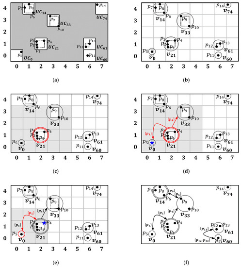
Figure 7 shows the step-by-step constructing process of the constraint graph$G\left(V, E\right)$when$\epsilon =\sqrt{2}$and$MinPts=3$for the sample dataset$P$, using an identical dataset to that shown in Figure 5. The example starts with a partitioned dataset,$\widehat{P}$, as shown in Figure 7a. First, as shown in Figure 7b, each$UC$is mapped into the vertices of$G$, and the unique identifier of each$UC$is used as the unique identifier of the vertex. Second, a vertex is selected by the input sequence of objects. In our case, a vertex$v_{21}$containing$p_1$is selected as shown in Figure 7c. To find the adjacent vertices for$v_{21}$, the$MRD$of$v_{21}$(i.e., gray area) is computed using Definition 4. Here, two vertices$v_0$and$v_{33}$are found as adjacent vertices of$v_{21}$. Next, the state of$v_{21}$,$v_{21}.vstate$, is obtained according to Definition 6. Here, all objects in$v_{21}$are$\epsilon$-core objects hence$v_{21}.vstate$is$stable$and depicted in a doubled circle. Third, as shown in Figure 7d, linkage constraints for$LC\left(v_{21}, v_0\right)$and$LC\left(v_{21}, v_{33}\right)$are obtained using Definition 5. For example, let the$MBR$of a vertex$v_i$be$v_i.MBR$. We first obtain the$\epsilon$-core objects of$v_{21}$, but we can skip this step because$v_{21}.vstate$is$stable$. Next, an$\epsilon$-core object of$v_{21}$closest to$v_0.MBR$,$p_1$, is obtained. Because$v_0$contains only one object, the coordinate of$v_0.MBR$farthest from$p_1$is$p_5$(blue star). Thus,$LC\left(v_{21}, v_0\right)$contains only$p_1$because no$\epsilon$-core object is closer to$p_5$than$p_1$. Then, because the constraint between$v_{21}$and$v_0$is defined, the two vertices are linked by$e\left(v_0, v_{21}\right)$. Figure 7e shows the linkage constraint$LC\left(v_0, v_{21}\right)$and state of$v_0$. The$v_0$contains only one object. Thus,$v_0.vstat\mathrm{e}$is$unstable$(circle) due to the adjacent vertex$v_{21}$that contains four objects.$LC\left(v_0, v_{21}\right)$contains$p_5$and thus$e\left(v_0, v_{21}\right)$becomes bidirectional. On the other hand,$v_{74}$contains only one object and has no adjacent vertex. Thus, the state of$v_{74}$is$noise$and is depicted as a dotted circle. When all vertices are processed, constraint graph $G$ is constructed, as shown in Figure 7f.

Figure 7. Construction of constraint graph $G\left(V, E\right)$ for sample dataset $P$ ($\epsilon =\sqrt{2}$ and $MinPts=3$): (a) the sample dataset $P$ partitioned into non-empty $UC$s, (b) vertices that are corresponding to $UC$s, (c) $MRD$ and $vstate$ of $v_{21}$, (d) edges in $v_{21}$. with linkage constraints weighted, (e) an edge in $v_0$ with a linkage constraint weighted, and (f) the constraint graph.

3.4. Plotting Step

In the plotting step, we traverse the constraint graph to generate a reachability plot as in OPTICS. Recall from Section 2.1.2 that OPTICS computes reachability distances for all pairs of objects to create a reachability plot. However, to create a reachability plot, only one reachability distance is required for each object. Through the constraint graph, we can reduce the reachability distance computations that do not contribute to generating the reachability plot. Here, the constraint graph identifies the reachability distance of each object required for the reachability plot by the linkage constraint. Thus, we reduce the unnecessary distance computations by only computing the distance between objects contained in the vertices which are linked to each other. We can further reduce the unnecessary distance computations by only computing the reachability distance for objects that satisfy the linkage constraints between the linked vertices. To plot a reachability plot, we traverse the constraint graph with the following rules: (i) if two objects are contained in the same vertex, the distance is computed; (ii) if two objects are contained in different vertices, only objects that satisfy the linkage constraint between two vertices are computed; (iii) the object with the closest reachability distance to the target object becomes the next target object; (iv) if no object is reachable, the next target object is selected by the input order of objects. For clarity, we provide the pseudocode, which will be referred to as the C-OPTICS procedure.

Algorithm 1: C-OPTICS

Input:   (1) $P=\left\{p_1, p_2, \cdots , p_n\right\}$: the input dataset   (2) $G\left(V, E\right)$: the constraint graph for $P$

Output:   (1) $RP$: a reachability plot

Algorithm:

Initialize the list $RP⟨object, rdist⟩$ and the priority queue $OrderSeed⟨object, rdist⟩$. foreach$p_{target}\in P$do   if $p_{target}.Unprocessed$ then    $p_{target}.Unprocessed=false$.    Put $p_{target}$ into $RP$.    $v_{target}=p_{target}$.get Vertex().    if $v_{target}.vstate\ne noise \& p_{target}$.iscore() then     Update $\left(p_{target},v_{target}, OrderSeed\right)$.     while $OrderSeed\ne \varnothing$ do      $p_{target}=OrderSeed$.next().      $p_{target}.Unprocessed=false$.      Put $p_{target}$ into $RP$.      $v_{target}=p_{target}$.get Vertex().      If $v_{target}.vstate\ne noise \& p_{target}$.iscore() then       Update$\left(p_{target}, v_{target}, OrderSeed\right)$. end

Algorithm 1 shows the C-OPTICS procedure that creates a reachability plot by traversing the constraint graph and plotting the reachability distance of each object. The inputs for C-OPTICS are the dataset $P$ and the constraint graph $G\left(V, E\right)$. The output of C-OPTICS is the reachability plot $RP$. In line 1, $RP$, a list structure representing the reachability plot, and $OrderSeed$, a priority queue structure, are initialized. Here, $OrderSeed$ determines the order in which to traverse the constraint graph. In line 2, a target object $p_{target}\in P$ is selected by the input order of objects. In line 3, the algorithm checks whether the target object $p_{target}$ has been processed. If $p_{target}$ is not processed, $p_{target}$ is set to the processed state in line 4. Then, $p_{target}$ is inputted to $RP$ with $UNDEFINED$ reachability distance (infinite). In line 6, the vertex $v_{target}\in V$, which contains $p_{target}$, is obtained. If $v_{target}.vstate$ is a $noise$, in line 7, $p_{target}$ is determined to be a noise object and the algorithm selects the next target object. If $v_{target}.vstate$ is not a $noise$, $p_{target}$ is checked as to whether $p_{target}$ is an $\epsilon$-core object. If $p_{target}$ is not an $\epsilon$-core object, $p_{target}$ is determined to be a noise object. In the opposite case, in line 8, the Update procedure is called to discover $N_{\epsilon }\left(p_{target}\right)$, after which $OrderSeed$ is updated. In lines 9–14, repeated processes are performed on $OrderSeed$. The object with the highest priority in $OrderSeed$ is selected as the next target object $p_{target}$ in line 10. Then, $p_{target}$ is set to the processed state in line 11. Next, in line 12, $p_{target}$ is inputted to $RP$ with the computed reachability distance. Then, a vertex $v_{target}$, which contains $p_{target}$, is obtained. In lines 13 and 14, $OrderSeed$ is updated by the Update procedure when $v_{target}.vstate$ is not $noise$ and $p_{target}$ is an $\epsilon$-core object. This process is repeated until $OrderSeed$ is empty. When $OrderSeed$ is empty, the unprocessed object is selected as the next target object $p_{target}\in P$. Thereafter, all of the above processes are repeated. When all objects are processed, $RP$ is output. Here, listing the objects in $RP$ results in a reachability plot.

Algorithm 2 shows the Update procedure that determines whether $OrderSeed$ is updated according to the state of each vertex and linkage constraints. The inputs for the Update are the object $p_{target}$, vertex $v_{target}$ containing $p_{target}$, and priority queue $OrderSeed$. The output of Update is $OrderSeed$. In line 1, $N_{\epsilon }\left(p_{target}\right)$ of $p_{target}$ is obtained. In line 2, an object $p_{neighbor}\in N_{\epsilon }\left(p_{target}\right)$ is selected. In line 3, the processing state of $p_{neighbor}$ is checked. When $p_{neighbor}$ is processed, a new object $p_{neighbor}\in N_{\epsilon }\left(p_{target}\right)$ is selected; otherwise, in line 4, a vertex $v_{neighbor}\in V$ containing $p_{neighbor}$ is obtained. In line 5, $p_{target}$ is checked for whether it satisfies the linkage constraint $LC\left(p_{target}, p_{neighbor}\right)$. If $p_{target}$ satisfies $LC\left(p_{target}, p_{neighbor}\right)$, the reachability distance of $p_{neighbor}$ to $p_{target}$ is computed and $OrderSeed$ is updated. In the opposite case, the reachability distance of $p_{neighbor}$ is not computed and thus $OrderSeed$ is not updated.

Algorithm 2: Update

Input:   (1) $p_{target}$: a target object of dataset $D$   (2) $v_{target}$: a target vertex of constraint graph $G$   (3) $OrderSeed$: a priority queue Output:   (4) $OrderSeed$: a priority queue

Algorithm:

$neighbors=p_{target}$.getNeighbors(${\epsilon }_{max}$, $MinPts$) foreach$p_{neighbor}\in neighbors$do   if $p_{neighbor}.Unprocessed$ then    $v_{neighbor}=p_{neighbor}$.get Vertex().    if $LC\left(v_{target},v_{neighbor}\right)$.con$\mathrm{tains}$($p_{target}$) then     $rdist=\max \left(p_{target}.cdist, dist\left(p_{target}, p_{neighbor}\right)\right)$.     $OrderSeed$.update$\left(p_{neighbor}, rdist\right)$. end

Example 3.

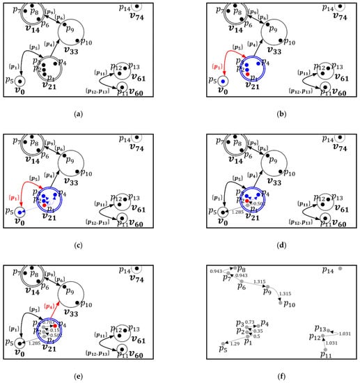
Figure 8 shows the step-by-step clustering process of the plotting step for the sample dataset$P$. Here, this example assumes that$\epsilon =\sqrt{2}$and$MinPts=3$, and a constraint graph$G\left(V, E\right)$is created, as shown inFigure 8a. First, a target object$p_i\in P$is selected by the input sequence of objects. Thus,$p_1$is selected (red dot), as shown inFigure 8b. Second, a vertex$v_{21}$containing$p_1$is obtained (blue circle) and the$\epsilon$-neighborhood of$p_1$,$N_{\epsilon }\left(p_1\right)$, is obtained (blue dots). Because$LC\left(v_{21}, v_0\right)$is satisfied,$p_5$contained in a vertex$v_0$is also a neighbor of$p_1$. Conversely, because$LC\left(v_{21}, v_{33}\right)$is not satisfied, two objects$p_9$and$p_{10}$contained in a vertex$v_{33}$are not neighbors of$p_1$. Third, as shown in Figure 8c, the reachability distance of each object, which is contained in$N_{\epsilon }\left(p_1\right)$, is computed for$p_1$according to Definition 2. Fourth, an object$p_2$having the closest reachability distance to$p_1$is selected as the next target object as shown in Figure 8d (red dot). Then, the above process is repeated for$p_2$. Note that only objects contained in$v_{21}$are considered because no linkage constraint is satisfied. Figure 8e shows the process for$p_4$. Where$p_4$satisfies$LC\left(v_{21}, v_{33}\right)$, however, two objects$p_9$and$p_{10}$are not neighbors of$p_4$because$dist\left(p_4, p_9\right)$and$dist\left(p_4, p_{10}\right)$are greater than$\epsilon$. Thus, the next target object is not selected. In this case, the next target object is selected by the input order of objects which are not processed. The above process is repeated for all unprocessed objects, creating a unidirectional graph structure that represents the reachability plot, as shown in Figure 8f.

Figure 8. An example of the plotting step for sample dataset $P$ ($\epsilon =\sqrt{2}$ and $MinPts=3$): (a) the constraint graph for the sample dataset $P$, (b) $N_{\epsilon }\left(p_1\right)$ that is obtained by using the linkage constraints of $p_1$, (c) the reachability distances of all objects contained in $N_{\epsilon }\left(p_1\right)$ for $p_1$, (d) the reachability distances of all objects contained in $N_{\epsilon }\left(p_2\right)$ for $p_2$, (e) $N_{\epsilon }\left(p_4\right)$, and (f) a unidirectional graph structure that represents the reachability plot.

4. Performance Evaluation

This section presents the experiments designed to evaluate C-OPTICS. The main purposes of these experiments are to provide experimental evidence that C-OPTICS alleviates the quadratic time complexity of OPTICS and that it outperforms the current state-of-the-art algorithms. Section 4.1 presents the meta-information pertaining to the experiments. Afterward, Section 4.2 shows the quality of a reachability plot by C- OPTICS and the running time achieved by C-OPTICS compared to the state-of-the-art algorithms.

4.1. Experimental Setup

This subsection describes the meta-information set up to perform the experiment. The experiments were run on a machine with a single core (Intel Core i7-8700 3.20 GHz CPU) and 48 GB of memory. The operating system installed is Windows 10 x64. All algorithms used in our experiments were implemented in the Java programming language. Moreover, the maximum Java heap memory in the JVM environment was set to 48 GB. Section 4.1.1 describes the datasets used in the experiments. Section 4.1.2 describes the existing algorithms which are compared with C-OPTICS. Section 4.1.3 describes the approach used to evaluate the clustering quality (accuracy of the reachability plot) of the algorithms.

4.1.1. Datasets

We conducted experiments with three real datasets and two synthetic datasets. The real datasets are termed HT, Household, and PAMAP2, and are obtained from the UCI Machine Learning Repository [26]. First, HT is a ten-dimensional dataset that collects measured values of home sensors that monitor the temperature, humidity, and concentration levels of various gases produced in another project [27]. Second, Household is a seven-dimensional dataset that collects the measured values of active energy consumed by each electronic product in the home. Third, PAMAP2 is a four-dimensional dataset that collects the measured values of three inertial forces and the heart rates for 18 physical activities produced during a project [28]. The Synthetic datasets are referred to here as BIRCH2 and Gaussian. First, BIRCH2 is a synthetic dataset for a clustering benchmark produced in earlier work [29]. This paper extended BIRCH2 to one million instances in seven dimensions to evaluate the dimensionality and scalability of the algorithms. Second, Gaussian is a synthetic dataset for the benchmarking of the clustering quality and the running time of the algorithms according to the size of the dimensions. It has a minimum of ten dimensions and a maximum of 50 dimensions. Table 2 presents the properties of all datasets, including their sizes and dimensions. In addition, each dataset was sampled at various sizes to assess the scalability of the algorithms.

Table 2. Meta-information of the datasets.

Dataset	Number of Instances	Number of Dims	Domain of Each Dims	Data Type
HT	928,991	10	[0,1]	Real
Household	2,049,280	7	[0,1]	Real
PAMAP2	3,850,505	4	[0,1]	Real
BIRCH2	1,000,000	7	[0,1]	Synthetic
Gaussian	500,000	10–50	[0,1]	Synthetic

4.1.2. Competing Algorithms

We compared C-OPTICS with the three state-of-the-art algorithms, each of which is representative in a unique sense, as explained below:

• OPTICS: The naïve algorithm [12] with the spatial indexing structure R*-tree to improve range queries;
• DeLi-Clu: A state-of-the-art algorithm that quickly creates an exact reachability plot by improving the single-linkage approach [15];
• SOPTICS: A fast OPTICS algorithm that achieves sub-quadratic time complexity by resorting to approximation using random projection [16].

Our comparisons with the above algorithms had different purposes. The comparisons with OPTICS and DeLi-Clu, which create an exact reachability plot, focus on evaluating the running time of C-OPTICS. As can be observed from the experimental results in Section 4.2, C-OPTICS is superior in terms of running time to both algorithms in all cases.

The comparison with SOPTICS represents the assessments of the clustering quality (accuracy of the reachability plot) and the running time. Here, the main purpose is to demonstrate two phenomena through experiments. First, the reachability plot created by C-OPTICS is robust and accurate in all cases, unlike that by SOPTICS. Second, C-OPTICS outperforms SOPTICS in terms of running time. These outcomes are verified in experimental results on the three real datasets and two synthetic datasets introduced in Section 4.1.1.

All four algorithms, including C-OPTICS, run in a single-threaded environment, with the selected parameter settings for each algorithm differing depending on the dataset. Table 3 lists the parameters of each algorithm and their search ranges.

Table 3. Parameters and search ranges for the three compared algorithms.

Algorithm	Parameters and Search Ranges
OPTICS	$\epsilon \in \left[0.2, 2.5\right];MinPts\in \left\{20, 30, 40, 50\right\}$
DeLi-Clu	$MinPts\in \left\{20, 30, 40, 50\right\}$
SOPTICS	$MinPts\in \left\{20, 30, 40, 50\right\}$
C-OPTICS	$\epsilon \in \left[0.2, 2.5\right];MinPts\in \left\{20, 30, 40, 50\right\}$

4.1.3. Clustering Quality Metrics

We assess the clustering quality of the algorithms with two approaches. The first seeks to present the reachability plots in full to enable a direct visual comparison. This approach, however, fails to quantify the degree of similarity. In addition, the larger the dataset size, the more difficult it is to observe the difference between the reachability plots. To remedy this defect, we use the adjusted Rand index (ARI) with 30-fold cross-validation.

ARI is a metric that evaluates the clustering quality based on the degree of similarity through all pair-wise comparisons between extracted clusters [30,31,32]. ARI returns a real value between 0 and 1, with 1 representing completely identical clustering. However, the reachability plot visualizes only the hierarchy of clusters without extracting the clusters. To measure the ARI of a reachability plot, we extract clusters for a reachability plot by defining the thresholds for ${\epsilon }_t$. Thus, ARI is computed by comparing the clusters of OPTICS with the clusters of each algorithm for ${\epsilon }_t$. In other words, the reachability plot of OPTICS is used as ground truth to evaluate the algorithms SOPTICS and C-OPTICS. In order to demonstrate the robustness of the clustering quality, the experiment is repeated and the computed minimum and maximum ARIs are compared.

4.2. Experimental Results

In this subsection, we present experimental evidence of the robustness of the clustering quality and the superior computational efficiency of C-OPTICS in a comparison with the three state-of-the-art algorithms OPTICS, DeLi-Clu, and SOPTICS. Section 4.2.1 describes the experimental results on the clustering quality of C-OPTICS and SOPTICS based on the two approaches used to evaluate the clustering quality introduced in Section 4.1.3. Section 4.2.2 presents the results of the experiments on scalability and dimensionality to evaluate the computational efficiency of C-OPTICS.

4.2.1. Clustering Quality

In this subsection, we present the robustness of the clustering quality of C-OPTICS through a comparison with OPTICS and SOPTICS. Here, DeLi-Clu is excluded from the evaluation of clustering quality because DeLi-Clu creates a reachability plot identical to that of OPTICS. Note that the clustering quality for each algorithm is evaluated on the basis of OPTICS as mentioned in Section 4.1.3. To assess the clustering quality according to the two approaches mentioned in Section 4.1.3, the reachability plots are directly compared first.

Figure 9 presents a visual comparison of the reachability plots for PAMAP2. Figure 9a–c show the reachability plots for OPTICS, C-OPTICS, and SOPTICS, respectively. The reachability plots for each algorithm are similar; however, many differences are observed based on the threshold ${\epsilon }_2$. Figure 9a,b show that four identical clusters ($C_1, C_2, C_3,$ and $C_4$) are extracted from OPTICS and C-OPTICS. On the other hand, Figure 9c shows that, unlike OPTICS, two clusters are extracted from SOPTICS. This result is due to the accumulation of deformations in the dataset by repeated random projection, which creates a reachability plot different from that by OPTICS. Conversely, C-OPTICS creates a reachability plot identical to that by OPTICS, as shown in Figure 9b, as it identifies the essential distance computations to guarantee an exact reachability plot.

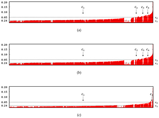
Figure 9. Visual comparison of reachability plots for PAMAP2: (a) OPTICS; (b) C-OPTICS; (c) SOPTICS.

Figure 10 shows ARI with respect to the value of $MinPts$ for each algorithm. Here, each dot on a curve gives the minimum ARI and is associated with a vertical bar that indicates the corresponding maximum ARI. This experiment compared the influence of $MinPts$ on ARI of each algorithm for three real datasets HT, Household, and PAMAP2, and one synthetic dataset BIRCH2. Figure 10 shows that C-OPTICS creates a reachability plot for all datasets. C-OPTICS guarantees that the reachability distance of each object is identical to OPTICS by linkage constraint and thus ARI of C-OPTICS is 1. This means that a reachability plot formed by C-OPTICS is identical to OPTICS. Furthermore, these results show that C-OPTICS is robust for $MinPts$ and is not dependent. SOPTICS creates different reachability plots for all datasets. Furthermore, the maximum and minimum ARI outcomes are influenced by the value of $MinPts$. In most cases, when $MinPts$ is small, the difference between the minimum and maximum ARI is large, as the smaller the value of $MinPts$ is, the more the random projection is performed, and the deformations can thus accumulate more. Figure 11 shows the ARI outcomes with respect to the number of dimensions for the Gaussian dataset. This experiment focuses on the dependence of the ARI of each algorithm on the number of dimensions. According to Figure 11, C-OPTICS guarantees ARI even if the number of dimensions increases. In other words, C-OPTICS creates a reachability plot identical to that by OPTICS regardless of the number of dimensions. The strategy for improving the computational efficiency of C-OPTICS is not dependent on the number of dimensions. However, as the number of dimensions increases, the minimum ARI decreases for SOPTICS. This occurs because the random projection of SOPTICS increases as the number of dimensions increases, as with $MinPts$. Thus, the difference between the minimum and maximum ARI becomes large, as shown in Figure 11.

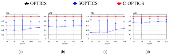
Figure 10. Clustering quality quantified by adjusted Rand index (ARI) vs. $MinPts$: (a) HT; (b) Household; (c) PAMAP2; (d) BIRCH2.

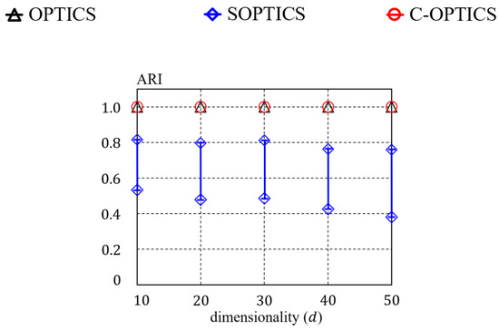
Figure 11. Clustering quality quantified by ARI vs. dimensionality for the Gaussian dataset.

4.2.2. Computational Efficiency

This subsection evaluates the computational efficiency of C-OPTICS and the three state-of-the-art algorithms using the three real datasets HT, Household, PAMAP2, and two synthetic datasets BIRCH2 and Gaussian (50 dimensions). Although there are distribution-based algorithms which improve the running time of OPTICS, this paper excludes those algorithms, as we do not consider a distributed environment. Figure 12 shows the result of the comparison of running time for each algorithm according to the sampled ratios for the two synthetic datasets. Note that the y-axis is presented on a logarithmic scale. In addition, if the running time of an algorithm exceeds ${10}^5$ s, it does not appear on the graph. This indicates that the algorithms did not terminate within 24 h and therefore were not considered for further experiments. As shown in Figure 12a, at a sampling rate of 5% for BIRCH2, C-OPTICS improved the running time by fivefold over OPTICS. As the sampling rate increases (i.e., as the size of the dataset increases), C-OPTICS improves the running times by up to 25 times over OPTICS. C-OPTICS even improved the running times by up to eight times over the fastest SOPTICS among the other algorithms. Figure 12b shows the results of the comparison for algorithm running times for the 50-dimensional Gaussian dataset. Here, C-OPTICS shows an improvement up to 100 times over OPTICS, as the efficiency of the spatial indexing structure at high dimensions is significantly decreased. These results also show a similar trend in the running time comparison with DeLi-Clu. For SOPTICS, which does not use a spatial indexing structure, a running time similar to that of C-OPTICS arises because it is not influenced by the number of dimensions. Similar trends were observed in the experiments on the three real datasets, as shown in Figure 13. As the sampling rate increased, the running time of C-OPTICS improved significantly compared to that by OPTICS. For the HT dataset in Figure 13a, C-OPTICS shows an improvement by as much as 50 times over OPTICS and up to nine times over SOPTICS. For the Household dataset in Figure 13b, the results for C-OPTICS are improved by up to 150 times over OPTICS. Conversely, C-OPTICS shows a running time nearly identical to that of SOPTICS. This corresponds to nearly identical worst case for C-OPTICS, where most of the objects are contained in a few vertices. Nevertheless, it is important to note that C-OPTICS shows an improvement over SOPTICS. Likewise, for the PAMAP2 dataset in Figure 13c, C-OPTICS overwhelms the other algorithms. These experimental results show that C-OPTICS outperforms the other algorithms in terms of computational efficiency.

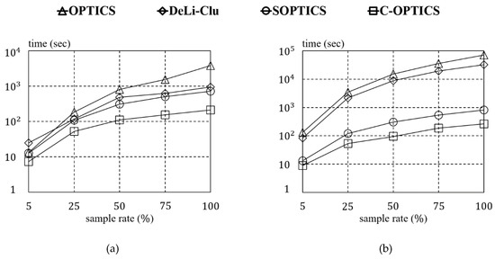
Figure 12. Running time vs. sampling rate for synthetic datasets: (a) BIRCH2; (b) Gaussian (50$d$).

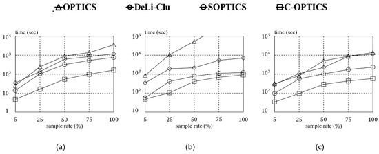
Figure 13. Running time vs. sampling rate for real datasets: (a) HT; (b) Household; (c) PAMAP2.

To provide an additional direct comparison of the running time for the algorithms, we compared the rate of reduction of the total number of distance computations for each algorithm with OPTICS. Figure 14 shows the experimental results for all datasets, where it can be observed that the total number of distance computations for C-OPTICS is significantly reduced. Again, it should be noted that the y-axis is presented on a logarithmic scale. C-OPTICS reduces the distance computations by more than ten times in all cases compared to OPTICS. This occurs because C-OPTICS identifies and excludes unnecessary distance computations based on the constraint graph.

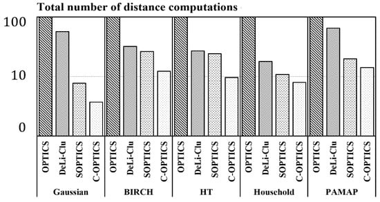
Figure 14. Comparison of the total number of distance computations.

We conducted experiments on Gaussian datasets of various dimensions to evaluate the dimensionality of C-OPTICS experimentally. Commonly, the running time also increases due to the number of dimensions, and the numbers of distance computations are proportional. Figure 15 shows linear time complexity regarding the number of dimensions for C-OPTICS as compared to SOPTICS. In contrast, OPTICS and DeLi-Clu show an exponential increase in the running time as the number of dimensions increases. Moreover, the computational efficiency of the algorithms decreases and the running time increases exponentially. As a result, C-OPTICS is shown to improve the scalability significantly and can address the quadratic time complexity of OPTICS while guaranteeing the quality of a reachability plot.

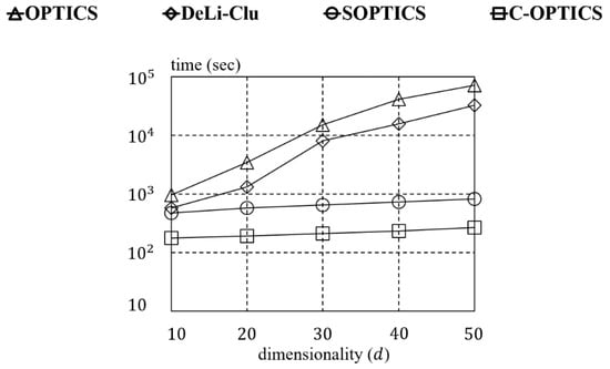
Figure 15. Running time vs. dimensionality for the Gaussian (50d) dataset.

5. Conclusions

In this paper, we proposed C-OPTICS, which improves the running time of OPTICS by reducing the unnecessary distance computations to address the quadratic time complexity issue of OPTICS. C-OPTICS partitions a $d$-dimensional dataset into unit cells which have identical diagonal length and constructs a constraint graph. Subsequently, C-OPTICS only computes the reachability distance for each object that appears in the reachability plot through linkage constraints in the constraint graph.

We conducted experiments on synthetic and real datasets to confirm the scalability and efficiency of C-OPTICS. Specifically, C-OPTICS outperformed state-of-the-art algorithms. Experimental results show that C-OPTICS addressed the quadratic time complexity of OPTICS. Specifically, the running time with regard to the data size is improved by as much as 102 times over DeLi-Clu. In addition, the running time is improved up to nine times over SOPTICS, which creates an approximate reachability plot. We also conducted experiments on dimensionality. These experimental results show that C-OPTICS has robust clustering quality and linear time complexity regardless of the size of the dimensions.

Future research can consider methods by which the proposed algorithm can be improved. For example, C-OPTICS can be improved by having it construct a constraint graph without depending on a radius $\epsilon$. This can provide a solution to the worst case of C-OPTICS. In addition, C-OPTICS can be improved to enable GPU-based parallel processing to accelerate the construction of the constraint graph.

References

- Wang, Z.; Yu, Z.; Chen, C.P.; You, J.; Gu, T.; Wong, H.S.; Zhang, J. Clustering by local gravitation. IEEE T. Cybern. 2017, 48, 1383–1396. [Google Scholar] [CrossRef] [PubMed]
- Li, Z.; Chen, J. Superpixel segmentation using linear spectral clustering. In Proceedings of the IEEE Conference on Computer Vision and Pattern Recognition, Boston, MA, USA, 7–12 June 2015; pp. 1356–1363. [Google Scholar]
- Fang, Z.; Yu, X.; Wu, C.; Chen, D.; Jia, T. Superpixel Segmentation Using Weighted Coplanar Feature Clustering on RGBD Images. Appl. Sci. 2018, 8, 902. [Google Scholar] [CrossRef]
- Torti, E.; Florimbi, G.; Castelli, F.; Ortega, S.; Fabelo, H.; Callicó, G.; Marrero-Martin, M.; Leporati, F. Parallel K-Means clustering for brain cancer detection using hyperspectral images. Electronics 2018, 7, 283. [Google Scholar] [CrossRef]
- Han, C.; Lin, Q.; Guo, J.; Sun, L.; Tao, Z. A Clustering Algorithm for Heterogeneous Wireless Sensor Networks Based on Solar Energy Supply. Electronics 2018, 7, 103. [Google Scholar] [CrossRef]
- Al-Shalabi, M.; Anbar, M.; Wan, T.C.; Khasawneh, A. Variants of the low-energy adaptive clustering hierarchy protocol: Survey, issues and challenges. Electronics 2018, 7, 136. [Google Scholar] [CrossRef]
- Panapakidis, I.P.; Michailides, C.; Angelides, D.C. Implementation of Pattern Recognition Algorithms in Processing Incomplete Wind Speed Data for Energy Assessment of Offshore Wind Turbines. Electronics 2019, 8, 418. [Google Scholar] [CrossRef]
- Zhang, T.; Haider, M.; Massoud, Y.; Alexander, J. An Oscillatory Neural Network Based Local Processing Unit for Pattern Recognition Applications. Electronics 2019, 8, 64. [Google Scholar] [CrossRef]
- Yaohui, L.; Zhengming, M.; Fang, Y. Adaptive density peak clustering based on K-nearest neighbors with aggregating strategy. Knowl. Based Syst. 2017, 133, 208–220. [Google Scholar] [CrossRef]
- Zaiane, O.R.; Foss, A.; Lee, C.H.; Wang, W. On data clustering analysis: Scalability, constraints, and validation. In Proceedings of the 6th Pacific-Asia Conference on Knowledge Discovery and Data Mining, Taipei, Taiwan, 6–8 May 2002; pp. 28–39. [Google Scholar]
- Ester, M.; Kriegel, H.P.; Sander, J.; Xu, X. A density-based algorithm for discovering clusters in large spatial databases with noise. In Proceedings of the 2nd International Conference on Knowledge Discovery and Data Mining, Portland, OR, USA, 2–4 August 1996; pp. 226–231. [Google Scholar]
- Ankerst, M.; Breunig, M.; Kriegel, H.P.; Sander, J. OPTICS: Ordering points to identify the clustering structure. In Proceedings of the ACM SIGMOD International Conference on Management of Data, Philadelphia, PA, USA, 1–3 June 1999; pp. 49–60. [Google Scholar]
- Patwary, M.A.; Palsetia, D.; Agrawal, A.; Liao, W.K.; Manne, F.; Choudhary, A. Scalable parallel OPTICS data clustering using graph algorithmic techniques. In Proceedings of the International Conference on High Performance Computing, Networking, Storage and Analysis, Denver, CO, USA, 17–22 November 2013; pp. 49–60. [Google Scholar]
- Gunawan, A.; de Berg, M. A Faster Algorithm for DBSCAN. Master’s Thesis, Eindhoven University of Technology, Eindhoven, The Netherlands, March 2013. [Google Scholar]
- Achtert, E.; Böhm, C.; Kröger, P. DeLi-Clu: Boosting robustness, completeness, usability, and efficiency of hierarchical clustering by a closest pair ranking. In Proceedings of the 10th Pacific-Asia Conference on Knowledge Discovery and Data Mining, Singapore, 9–12 April 2006; pp. 119–128. [Google Scholar]
- Schneider, A.; Vlachos, M. Scalable density-based clustering with quality guarantees using random projections. Data Min. Knowl. Discov. 2017, 31, 972–1005. [Google Scholar] [CrossRef]
- Beckmann, N.; Kriegel, H.P.; Schneider, R.; Seeger, B. The R*-tree: An efficient and robust access method for points and rectangles. In Proceedings of the ACM SIGMOD International Conference on Management of Data, Atlantic City, NJ, USA, 23–25 May 1990; pp. 322–331. [Google Scholar]
- Brecheisen, S.; Kriegel, H.P.; Pfeifle, M. Multi-step density-based clustering. Knowl. Inf. Syst. 2006, 9, 284–308. [Google Scholar] [CrossRef][Green Version]
- Lee, W.; Loh, W.K. G-OPTICS: Fast ordering density-based cluster objects using graphics processing units. Int. J. Web Grid Serv. 2018, 14, 273–287. [Google Scholar] [CrossRef]
- Breunig, M.M.; Kriegel, H.P.; Sander, J. Fast hierarchical clustering based on compressed data and optics. In Proceedings of the 4th European Conference on Principles of Data Mining and Knowledge Discovery, Lyon, France, 13–16 September 2000; pp. 232–242. [Google Scholar]
- Vágner, A. The GridOPTICS clustering algorithm. Intell. Data Anal. 2016, 20, 1061–1084. [Google Scholar] [CrossRef]
- Stuetzle, W. Estimating the cluster tree of a density by analyzing the minimal spanning tree of a sample. J. Classif. 2003, 20, 25–47. [Google Scholar] [CrossRef]
- Hartigan, J.A.; Mohanty, S. The runt test for multimodality. J. Classif. 1992, 9, 63–70. [Google Scholar] [CrossRef]
- Campello, R.J.; Moulavi, D.; Zimek, A.; Sander, J. Hierarchical density estimates for data clustering, visualization, and outlier detection. ACM Trans. Knowl. Discov. Data 2015, 10, 5–56. [Google Scholar] [CrossRef]
- Bryant, A.; Cios, K. RNN-DBSCAN: A density-based clustering algorithm using reverse nearest neighbor density estimation. IEEE Trans. Knowl. Data Eng. 2018, 30, 1109–1121. [Google Scholar] [CrossRef]
- Blake, C.; Merz, C. UCI Repository of Machine Learning Database; UCI: Irvine, CA, USA, 1998. [Google Scholar]
- Huerta, R.; Mosqueiro, T.; Fonollosa, J.; Rulkov, N.F.; Rodriguez-Lujan, I. Online decorrelation of humidity and temperature in chemical sensors for continuous monitoring. Chemom. Intell. Lab. Syst. 2016, 157, 169–176. [Google Scholar] [CrossRef]
- Reiss, A.; Stricker, D. Introducing a new benchmarked dataset for activity monitoring. Proceedings of International Symposium on Wearable Computers, Boston, MA, USA, 11–15 November 2012; pp. 108–109. [Google Scholar]
- Zhang, T.; Ramakrishnan, R.; Livny, M. BIRCH: An efficient data clustering method for very large databases. In Proceedings of the ACM SIGMOD International Conference on Management of Data, Montreal, QC, Canada, 4–6 June 1996; pp. 103–114. [Google Scholar]
- Rand, W.M. Objective criteria for the evaluation of clustering methods. J. Am. Stat. Assoc. 1971, 66, 846–850. [Google Scholar] [CrossRef]
- Hubert, L.; Arabie, P. Comparing partitions. J. Classif. 1985, 2, 193–218. [Google Scholar] [CrossRef]
- Vinh, N.X.; Epps, J.; Bailey, J. Information theoretic measures for clustering comparison: Variants, properties, normalization and correction for chance. J. Mach. Learn. Res. 2010, 11, 2837–2854. [Google Scholar]
© 2019 by the authors. Licensee MDPI, Basel, Switzerland. This article is an open access article distributed under the terms and conditions of the Creative Commons Attribution (CC BY) license (http://creativecommons.org/licenses/by/4.0/).