Link Prediction Using Temporal Graph Neural Network Model

Abstract

In this work, we present a Temporal Graph Neural Network (TGNN) architecture specifically designed for link prediction in dynamic graphs. The proposed approach is evaluated on a dynamic social network constructed from internal email communication between employees of Wrocław University of Science and Technology that was collected over a continuous period of 605 days. To capture short-term fluctuations in communication behavior, we introduce the use of very short temporal aggregation windows, down to a single day, for constructing temporal graph snapshots. This fine-grained temporal resolution allows the model to accurately learn evolving interaction patterns and adapt to the dynamic nature of social communication networks. The TGNN model demonstrates consistently high predictive performance, achieving 99.28% ROC-AUC (Receiver Operating Characteristic—Area Under Curve) and 99.17% Average Precision in link prediction tasks. These results confirm that the model is able to distinguish between existing and emerging communication links with high reliability across temporal intervals. The architecture, optimized exclusively for temporal link prediction, effectively utilizes its representational capacity for modeling edge formation processes in time-dependent networks. The findings highlight the potential of focused TGNN architectures and short-time-window modeling in improving predictive accuracy and temporal resolution in link prediction applications involving evolving social or organizational structures.

1. Introduction and Related Work

The basic properties of social networks created from data gathered by modern information systems are complexity and dynamics. Here, complexity is understood in a general sense as the presence of non-trivial structural patterns and heterogeneous connectivity, without assuming any specific generative model. In classic social network models, relations tend to be stable, and they do not rapidly change over time. In technology-based social networks built on the basis of interactions occurring within information systems, we experience fast changes in the structural properties of the network. In the dataset used in this work, sometimes 30% of the links disappear between two consecutive time windows. Thus, structural changes are very difficult to investigate in terms of traditional social network analysis, which employs measures that are designed to effectively cope with static networks of small to average size.

Social networks created from data contain relations that are the result of a set of discrete events (like emails, phone calls, interactions with Web resources, blog entries, etc.) about which information is available. Because these events have some distribution, this adds a new dimension to the known problems of network analysis [1]. It can be shown that human activity related to communication and message exchanging may be characterized by short “bursts” of activity followed by longer periods of inactivity [2]. This phenomenon has significant consequences for traditional social network analysis. The standard methodology is to divide available data into timeframes (time windows), construct social networks corresponding to those windows, and then apply social network analysis to each time window separately. If the size of the time window is small, the bursty behavior of the users may lead to violent changes in the values of any structural measure (node degree, node centrality, node type, etc.) between consecutive time windows. We experience a trade-off—short time windows mean drastic changes in structural parameters, while long time windows give us less chances to capture the dynamics of the network [3,4]. In this study, we focus specifically on the problem of temporal link prediction in highly dynamic communication networks, where interactions occur as short, burst-like events. This setting differs fundamentally from static or slowly evolving networks and requires models capable of capturing fine-grained temporal patterns rather than relying on aggregated time window snapshots. A number of methods to address this problem have been developed, ranging from classical network-based techniques to machine learning approaches for predicting structural changes in dynamic networks [5,6]. They are used to effectively solve the “link prediction problem”, for they can estimate the probability that a certain link between network nodes will emerge/disappear when we move between consecutive time windows [7]. The goal of this work is to investigate whether a temporal graph neural network can effectively learn local structural evolution patterns from historical communication data and use them to predict future link occurrences. By integrating structural and temporal information, TGNN provides a flexible framework that, in contrast to traditional link prediction approaches, can improve predictive performance. We aim to evaluate the feasibility of this approach in a real, rapidly changing email-based network. Recent comprehensive surveys of temporal link prediction methods [8] and their theoretical foundations describe and organize existing approaches into transductive and inductive categories for modeling dynamic interactions [9]. A machine learning approach to the link prediction problem was proposed and tested in [10], while a multi-layer temporal network model was analyzed in [11].

The classic work [12] presents a broad survey and evaluation of link prediction algorithms. It also shows that the best predictors detect less than 10% of emerging links. The datasets used in experiments (like the arxiv co-authors’ social network) are also significantly more static than typical social networks built from email logs, which are highly dynamic in short timescales [13].

The contributions of this paper are twofold. First, we propose an application of a Temporal Graph Neural Network (TGNN) model to a real-world, high-frequency email communication network, which differs from typical benchmark datasets used in prior work in terms of high temporal volatility, the frequent emergence and disappearance of links, and the bursty nature of interactions. Second, we provide an empirical evaluation of TGNN’s performance in predicting both emerging and disappearing links, illustrating its capability to model rapid temporal fluctuations inherent in such communication environments. This phenomenon has motivated our application of neural networks to the link prediction problem within the Temporal Graph Neural Network (TGNN) model. This is supported by existing applications of neural graph learning, for example, in transport and logistics [14]. The motivation is to train the neural network using historic network data in order to learn about typical patterns of change in local network topology. A similar approach was also suggested in [8].

2. Model Architecture

Section 2 presents the architecture of the proposed NGLP model. The design emphasizes simplicity and interpretability, combining lightweight structural features with learnable node representations to model temporal link formation in dynamic directed graphs. Each component is intentionally kept modular, allowing the contribution of individual architectural choices to be clearly analyzed in later experiments.

2.1. Problem and Notation

We study the problem of temporal link prediction in dynamic directed networks, where interactions between users evolve over time. To capture these dynamics in a structured manner, the network is modeled as a sequence of discrete temporal snapshots, each representing interactions observed within a fixed time window. We consider a dynamic directed graph represented as a sequence of temporal snapshots:

$$\mathcal{G}=\{G_t=(V,E_t){\}}_{t=1}^T,$$

where $V$ is a fixed set of nodes (users) and $E_t\subseteq V\times V$ are directed edges observed within time window $t$(no self-loops, i.e., $u\ne v$).

The temporal link prediction $p_{uv}^{\left(t\right)}$ task is for each ordered pair $(u,v)$ to estimate the probability that an edge between $u$ and $v$ will appear in the next snapshot of the dynamic network:

$$p_{uv}^{\left(t\right)}\approx \mathrm{P}\mathrm{r}((u,v)\in E_{t+1}| G_t).$$

This formulation explicitly captures the one-step-ahead temporal dependency that is central to dynamic link prediction.

2.2. Snapshot Construction

The temporal modeling of communication networks requires an explicit representation of how interactions evolve over time. In the analyzed email datasets, interactions are recorded as individual, time-stamped events. While such an event-level representation preserves full temporal information, it is not directly suitable for temporal graph neural networks, which operate on sequences of graph-structured inputs. Therefore, a transformation from event streams to graph snapshots is necessary.

In this study, time-stamped email events are aggregated into a sequence of non-overlapping windows of length $d\in \left\{\mathrm{1,3},7\right\}$ days, producing an ordered sequence of edge sets $\left\{E_t\right\}$. The time window lengths of 1, 3, and 7 days were selected to capture different levels of temporal granularity in the communication data: 1-day windows allow the model to track fine-grained fluctuations, 3-day windows capture short-term patterns, and 7-day windows provide a coarser overview of trends. This choice balances the need to reflect bursty, high-frequency interactions with the stability of structural measures across consecutive snapshots. The use of multiple window lengths allows us to examine communication dynamics at different temporal resolutions. Short windows capture transient and bursty interaction patterns, whereas longer windows emphasize more stable and recurring communication relationships. From a practical perspective, this choice represents a reasonable compromise between temporal resolution and computational complexity, which is particularly important when working with long observation periods. To maintain consistency across experiments, the same snapshot construction procedure and window sizes are applied to the public datasets (email-Eu-core-temporal [15] and CollegeMsg [16]). For each temporal window, a directed graph snapshot is constructed, reflecting the inherently asymmetric nature of email communication. Self-loops are removed, as they do not carry meaningful relational information and may artificially inflate node connectivity measures. In preliminary experiments, retaining self-loops did not lead to improved performance and increased the variance of degree-based features.

Within each snapshot, basic structural characteristics of nodes are described using degree-related statistics. We use the notation deg(v) to indicate the degree (in- or out-degree) of node $v$ at time $t$. These graph snapshots constitute the fundamental input to the temporal graph neural network and provide the basis for learning node representations that evolve over time in subsequent stages of the proposed framework. From the modeling perspective, this representation offers a clear and interpretable link between raw communication events and learned temporal embeddings. This construction strikes a balance between temporal resolution and statistical stability. Short windows preserve fine-grained dynamics, while longer windows reduce sparsity, allowing us to assess how temporal aggregation influences link predictability within a unified architectural framework.

2.3. Node Representation

Node representations serve as the interface between the evolving graph structure and the temporal neural network. In this work, we combine simple degree-based structural descriptors with learnable node embeddings to capture both local connectivity patterns and latent, node-specific properties that are not directly observable from the graph topology. For each snapshot $G_t$, we compute degree-based structural features:

$$x_t^{deg}\left(v\right)=\left[\log \left(1+{\mathrm{deg}}_t^{\mathrm{in}}\left(v\right)\right),\mathrm{ }\log \left(1+{\mathrm{deg}}_t^{\mathrm{out}}\left(v\right)\right),\mathrm{ }\log \left(1+{\mathrm{deg}}_t^{\mathrm{in}}\left(v\right)+{\mathrm{deg}}_t^{\mathrm{out}}\left(v\right)\right)\right]\in R^3.$$

Each node also has a learnable embedding $\mathbf{e}(v)\in {\mathbb{R}}^{d_e}$ with $d_e=64$. The encoder input is the concatenation:

$$X_t\left(v\right)=\left[\mathbf{e}\left(v\right)|x_t^{\mathrm{d}\mathrm{e}\mathrm{g}}\left(v\right)\right]\in R^{d_e+3}.$$

This design allows the model to jointly exploit explicit structural information and flexible latent representations within a unified encoding framework. This hybrid representation allows the model to remain interpretable while retaining sufficient expressive power for complex temporal patterns.

2.4. Encoder: Two-Layer GCN

The role of the encoder is to transform raw node features and local graph structure into compact latent representations that can be propagated across time. For each snapshot, we employ a two-layer Graph Convolutional Network (GCN) to aggregate neighborhood information and capture higher-order structural dependencies within the graph.

Let ${\tilde{A}}_t=A_t+I$ and ${\tilde{D}}_t$ be the degree matrix of ${\tilde{A}}_t$. We use the normalized adjacency ${\widehat{A}}_t={\tilde{D}}_t^{-{\displaystyle \frac{1}{2}}}{\tilde{A}}_t{\tilde{D}}_t^{-{\displaystyle \frac{1}{2}}}$. The two GCN layers [17,18] are

$$H_t^{\left(1\right)}=\mathrm{R}\mathrm{e}\mathrm{L}\mathrm{U} \left({\widehat{A}}_t{X}_t{W}_1\right),Z_t={\widehat{A}}_t\hspace{0.17em}\mathrm{D}\mathrm{r}\mathrm{o}\mathrm{p}\mathrm{o}\mathrm{u}\mathrm{t}\hspace{0.17em}\left(H_t^{\left(1\right)}\right)\hspace{0.17em}{W}_2,$$

with $W_1\in {\mathbb{R}}^{(d_e+3)\times h}$, $W_2\in {\mathbb{R}}^{h\times h}$, and hidden size $h=128$. The matrix $Z_t\in {\mathbb{R}}^{\mid V\mid \times h}$ contains node embeddings at time $t$. These snapshot-level embeddings serve as the input to the temporal modeling component, enabling the network to learn how node representations evolve over successive time steps. Although the GCN operates on individual snapshots, temporal dependencies are implicitly modeled by applying the same encoder across consecutive snapshots and training the model to predict future links. These snapshot-level embeddings are then fed sequentially into the temporal component of the model, explicitly capturing temporal dependencies across consecutive snapshots to form the TGCN representation.

2.5. Decoder and Edge Scoring

The decoder maps pairs of node embeddings into a scalar score that reflects the likelihood of a directed interaction between two nodes. The input to the decoder consists of the node embeddings generated by the TGCN, and the output is a probability for each node pair indicating the likelihood of a directed edge in the next temporal snapshot. For each ordered node pair $(u,v)$, the corresponding snapshot-level embeddings are combined and passed through a two-layer multilayer perceptron (MLP) to compute an edge score.

A two-layer MLP produces a scalar logit:

$$s_{uv}^{\left(t\right)}=w_2^{\mathrm{\top }}\hspace{0.17em}\mathrm{D}\mathrm{r}\mathrm{o}\mathrm{p}\mathrm{o}\mathrm{u}\mathrm{t}\hspace{0.17em}\left(\mathrm{R}\mathrm{e}\mathrm{L}\mathrm{U}\hspace{0.17em}\left(W\hspace{0.17em}{\mathbf{g}}_{uv}^{\left(t\right)}\right)\right),$$

with $W\in {\mathbb{R}}^{2h\times h}$ and $w_2\in {\mathbb{R}}^h$. The predicted probability is

$$p_{uv}^{\left(t\right)}=\sigma \hspace{0.17em}(s_{uv}^{\left(t\right)}).$$

The resulting probability $p_{uv}^{\left(t\right)}$ is interpreted as the model’s confidence that a directed edge from $u$ to $v$ will appear in the next temporal snapshot. Together, the encoder–decoder design enables the model to jointly capture local structural context and asymmetric node roles, which are essential in directed communication networks such as email graphs.

2.6. Training with Negative Sampling

To train the model for temporal link prediction, we formulate the task as a binary link existence prediction problem over observed and unobserved edges between consecutive snapshots. Because the number of non-existing edges vastly exceeds the number of observed interactions, negative sampling is employed to construct a balanced and computationally tractable training set. The training uses consecutive pairs $(G_t,G_{t+1})$. Positives are all edges in $E_{t+1}$. Negatives are uniformly sampled non-edges $(u,v)\notin E_{t+1}$, where $u\ne v$, at a 1:1 negative-to-positive ratio. This negative sampling strategy ensures a balanced training set and reduces computational load while maintaining representative non-edge examples for effective link prediction. The loss is the binary cross-entropy with logits:

$$\mathcal{L}={\displaystyle \frac{1}{\mid {\mathcal{P}}_t\mid +\mid {\mathcal{N}}_t\mid }}\hspace{0.17em}\sum _{\left(u,v\right)\in {\mathcal{P}}_t\cup {\mathcal{N}}_t}\mathrm{B}\mathrm{C}\mathrm{E}\mathrm{W}\mathrm{i}\mathrm{t}\mathrm{h}\mathrm{L}\mathrm{o}\mathrm{g}\mathrm{i}\mathrm{t}\mathrm{s}\hspace{0.17em}\left(s_{uv}^{\left(t\right)},\hspace{0.17em}{y}_{uv}\right),$$

where $y_{uv}=1$ for $(u,v)\in {\mathcal{P}}_t=E_{t+1}$ and $y_{uv}=0$ for $(u,v)\in {\mathcal{N}}_t$.

The model parameters are optimized using standard stochastic gradient-based training settings commonly adopted in temporal graph learning.

For optimization, the following settings are used: Adam (learning rate ${10}^{-3}$), weight decay ${10}^{-4}$, dropout $0.3$, and early stopping on validation AP (patience $10$, max $50$ epochs). The random seed is $42$. The training uses GPU when available. These hyperparameter values were chosen based on standard practice in temporal graph learning and validated through preliminary experiments to ensure stable and effective training.

2.7. Decision Threshold Selection

To convert predicted probabilities into binary link existence decisions, a decision threshold is required. Rather than using an arbitrary fixed value, the threshold is selected in a data-driven manner based on validation performance. We select the decision threshold $\tau$ only on the validation set by maximizing $F_1$:

$${\tau }^{\star }=\mathrm{a}\mathrm{r}\mathrm{g}\underset{\tau \in \left[\mathrm{0,1}\right]}{\mathrm{m}\mathrm{a}\mathrm{x}}{F}_1\hspace{0.17em}(\mathbf{1}\{p_{uv}\ge \tau \},\hspace{0.17em}{y}_{uv}).$$

The chosen ${\tau }^{\star }$ is then fixed for test evaluation. This approach provides a balanced trade-off between precision and recall while ensuring a fair evaluation protocol.

2.8. Evaluation Metrics

To evaluate the behavior of the proposed architecture, we employ complementary metrics that capture both ranking quality and binary decision accuracy. Specifically, ROC-AUC and Average Precision assess the quality of edge ranking, while $F_{1 }$ and Precision@K quantify performance under a fixed decision threshold. We report ROC-AUC, Average Precision (AP), $F_{1 }$ at ${\tau }^{\star }$, and Precision@K, with

$$K=\mid {\mathcal{P}}_t\mid$$

equal to the number of positives in the test fold for $(t,t+1)$. We additionally record TP/FP/FN at ${\tau }^{\star }$. Temporal folds are split approximately 70/15/15 into train/validation/test by time order.

2.9. Baselines and Comparative Models Used for Evaluation

To provide a comprehensive evaluation, we compare the proposed model against classical heuristic-based link prediction methods as well as representative neural network–based approaches. Given the undirected projection of $G_t$ for scoring, we compute

• Common Neighbors (CN):

$$\mathrm{C}\mathrm{N}(u,v)=\mid \Gamma \left(u\right)\cap \Gamma \left(v\right)\mid .$$

2.

Adamic-Adar (AA):

$$\mathrm{A}\mathrm{A}(u,v)=\sum _{w\in \Gamma \left(u\right)\cap \Gamma \left(v\right)}{\displaystyle \frac{1}{\mathrm{l}\mathrm{o}\mathrm{g} \mathrm{d}\mathrm{e}\mathrm{g}\left(w\right)}}.$$

3.

Resource Allocation (RA):

$$\mathrm{R}\mathrm{A}(u,v)=\sum _{w\in \Gamma \left(u\right)\cap \Gamma \left(v\right)}{\displaystyle \frac{1}{\mathrm{d}\mathrm{e}\mathrm{g}\left(w\right)}}.$$

4.

Preferential Attachment (PA):

$$\mathrm{P}\mathrm{A}(u,v)=\mathrm{d}\mathrm{e}\mathrm{g}\left(u\right)\cdot \mathrm{d}\mathrm{e}\mathrm{g}\left(v\right).$$

Each score is min–max normalized to $\left[\mathrm{0,1}\right]$. We evaluate ROC-AUC and AP on the same candidate set (all positives from $E_{t+1}$ plus sampled negatives).

The following additional GNN-based comparative models were used:

• GAE-GCN [15]: Two GCN layers on learnable node embeddings $\mathbf{e}\left(v\right)$ and inner-product decoder $⟨Z\left(u\right),Z\left(v\right)⟩$.
• GraphSAGE Link Predictor [19]: Two SAGE layers, MLP decoder on $\left[Z\right(u)\parallel Z(v\left)\right]$, and loss and evaluation identical to NGLP (Next Graph Link Prediction).

2.10. Implementation and Reproducibility

We used the following libraries: PyTorch (v. 2.7.1) [20]; PyTorch Geometric (v. 2.6.1) [21] (GCN, SAGE layers); scikit-learn (v. 1.7.1) [22] (metrics); and NetworkX (v. 3.5) [23] (structural baselines).

The NGLP hyperparameters were as follows: $h=128$, $d_e=64$, dropout $0.3$, LR ${10}^{-3}$, weight decay ${10}^{-4}$, epochs $\le 50$, patience $10$, negative:positive $=1:1$, and seed $42$.

For the temporal split, if $T$ is the number of $(t,t+1)$ pairs, the validation uses $\mathrm{m}\mathrm{a}\mathrm{x}(1,\lfloor 0.15T\rfloor )$, the test uses $\mathrm{m}\mathrm{a}\mathrm{x}(1,\lfloor 0.15T\rfloor )$, and the remainder is training, preserving chronological order.

2.11. Pseudocode (Outline)

Algorithm 1 summarizes the complete training and evaluation pipeline implied by the proposed architecture.

Algorithm 1: Training and Evaluation of NGLP

Build snapshots $\{G_t{\}}_{t=1}^T$ with $d\in \{\mathrm{1,3},7\}$ days. Split $(t,t+1)$ pairs into ≈70/15/15 train/val/test by time. Training (per epoch): (a) For $t=1\dots T-1$: compute degree features $x_t^{\mathrm{deg}}$ and node states $Z_t$ (2-layer GCN); (b) Define ${\mathcal{P}}_t=E_{t+1}$ and sample ${\mathcal{N}}_t$(1:1); (c) Compute logits $s_{uv}^{\left(t\right)}$ and minimize $\mathcal{L}$; (d) Early stopping on validation AP. Validation: Choose ${\tau }^{\star }=\mathrm{a}\mathrm{r}\mathrm{g} {\mathrm{m}\mathrm{a}\mathrm{x}}_{\tau }{F}_1$. Test: Report ROC-AUC, AP, $F_1\left({\tau }^{\star }\right)$, Precision@K (with $K=\mid {\mathcal{P}}_t\mid$), and the chosen ${\tau }^{\star }$.

2.12. NGLP Architecture

Figure 1 illustrates the NGLP pipeline: Email events are aggregated into 1/3/7-day windows to form graph snapshots. Each node combines a learnable embedding with simple degree features; a two-layer GCN produces node representations. Directed pairs are scored by a small MLP on the concatenated source–target vectors to yield the next-snapshot link probability. The training uses positives from $t+1$ and uniformly sampled non-edges (1:1), with early stopping and a validation-selected decision threshold.

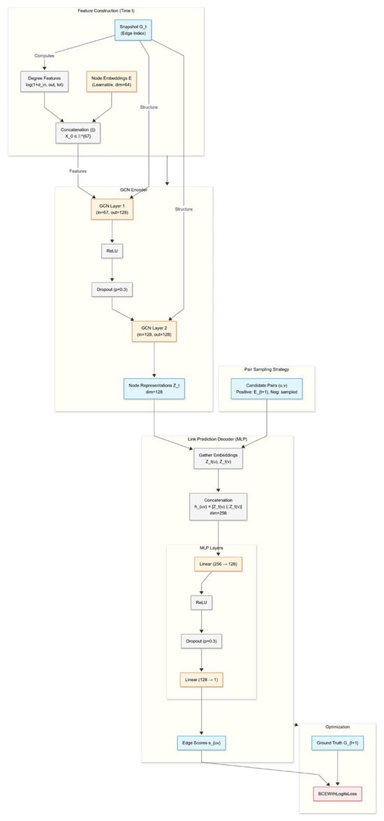
Figure 1. NGLP Architecture. Color coding: Blue nodes represent data tensors, orange nodes indicate learnable layers, grey nodes denote operations, and the red node represents the loss function.

3. Dataset Characteristics and Preprocessing

The dataset contains anonymized email exchanges between employees of Wrocław University of Technology (WUST), creating a useful communication network. Similar email datasets are often used in temporal graph learning research [24,25]. For example, the Stanford SNAP collection includes the email-Eu-core-temporal dataset, which has 986 nodes and 332,334 edges collected over 803 days from a European research institution [24].

In our former experiments we have analyzed the local topology of a number of communication-based social networks, including an email-based social network of employees of WUST containing 5834 nodes (email addresses) and 136,830 directed links (formed as a result of sending emails) [26].

To start experiments, WUST email logs were cleaned by removing any external communication, leaving only emails exchanged between staff members. The final dataset was built based on communication data from 605 days, and, in our experiments, was divided into time windows of 1, 3, and 7 days. This allowed us to create dynamic network models which were used to test our link prediction approach.

Figure 2 presents a visualization of the entire WUST email-based social network, based on the data gathered during the entire 605-day-long period of data gathering.

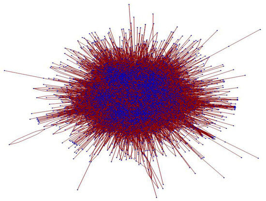
Figure 2. WUST email social network graph (5834 nodes and 136,830 links).

We observed significant structural changes in the networks corresponding to consecutive time windows, specifically, quite low link stability: 53% for 7-day time windows and only 42% for 1-day time windows (meaning that only 42% of the links observed in a given time window will be present in the next). This issue implies that our dataset is quite challenging for traditional link prediction methods based on structural approaches (Common Neighbour, Preferential Attachment, Katz predictors, etc.). Carrying out the the methods described above yielded the maximum number of new links predicted at ~5%, which strongly suggests the need for using of any type of machine learning algorithms capable of identifying complex patterns of link emergence. Even simple approaches based on statistics of local graph topology changes return satisfactory results, which was shown in [27], where a link predictor based on statistics of connection changes within triads of nodes was proposed. The neural graph-based approach applied in this work stems from these observations, which are further supported by other studies [28,29], showing that neural models offer a prospective approach to the link prediction problem in complex networks.

4. Experiments

4.1. Experimental Setup

The experimental evaluation follows the architectural design introduced in Section 2. That is, the same encoder–decoder pipeline is used across all temporal folds, while hyperparameters and training details are fixed to ensure reproducibility and fair comparison with baseline methods. We evaluate temporal link prediction from $G_t$ to $G_{t+1}$ using disjoint time ranges for train/validation/test (≈70/15/15). For each test pair $(t,t+1)$, positives are all directed edges in $E_{t+1}$; negatives are uniformly sampled non-edges (no self-loops) at a 1:1 ratio. We report ROC-AUC, Average Precision (AP), F1 at the validation-selected threshold, and Precision@K with $K$ equal to the number of positives in the test fold. Thresholds are chosen on validation to maximize F1 and then held fixed on test. The results below correspond to seed 42 and early stopping on validation AP (patience 10, max 50 epochs). The baselines are classical structural scores computed on the previous snapshot $G_t$ using Common Neighbors (CN), Adamic-Adar (AA), Resource Allocation (RA), and Preferential Attachment (PA).

For our datasets, we use the WUST email network with 1-day/3-day/7-day windows, and the public benchmarks email-Eu-core-temporal [15] and CollegeMsg [16], each with the same window sizes.

The selected baselines are intended to represent well-established and widely adopted graph-learning paradigms rather than the most recent task-specific architectures. This choice allows for a controlled comparison under a unified temporal evaluation protocol, which is often not directly comparable across recent works due to differences in data splits, sampling strategies, and evaluation setups.

4.2. Results on WUST (Local Snapshots)

The proposed model achieves consistently strong performance across all temporal resolutions (Table 1). Prediction quality is highest for shorter time windows (1-day and 3-day), which is reflected in higher AP and F1 scores, while performance gradually decreases for longer aggregation windows (7-day), where link dynamics become more stable but less informative for short-term prediction.

Table 1. Results for WUST.

Window	ROC-AUC	AP	F1	P@K	Thr
1-day	0.9929	0.9918	0.9628	0.9627	0.5747
3-day	0.9863	0.9840	0.9467	0.9454	0.4873
7-day	0.9789	0.9744	0.9289	0.9299	0.7222

The table below lists the structural baselines (best per window). Preferential Attachment (PA) is the strongest of the four, yet is far below NGLP (Table 2).

Table 2. Structural baselines.

Window	Best Baseline	ROC-AUC	AP
1-day	PA	0.8567	0.8598
3-day	PA	0.8448	0.8448
7-day	PA	0.8596	0.8564

4.3. Results on Public Benchmarks

4.3.1. Email-Eu-Core-Temporal

The performance metrics obtained for the email-Eu-core-temporal dataset are summarized in Table 3.

Table 3. Results for email-Eu-core-temporal.

Window	ROC-AUC	AP	F1	P@K	Thr	Best Baseline (ROC/AP)
1-day	0.9700	0.9617	0.9160	0.9125	0.5000	PA: 0.7056/0.6997
3-day	0.9688	0.9640	0.9044	0.9113	0.5000	PA: 0.6472/0.6588
7-day	0.9525	0.9394	0.8972	0.8936	0.5000	PA: 0.5235/0.5235

4.3.2. CollegeMsg

The experimental results for the CollegeMsg benchmark dataset are presented in Table 4.

Table 4. Results for CollegeMsg.

Window	ROC-AUC	AP	F1	P@K	Thr	Best Baseline (ROC/AP)
1-day	0.9957	0.9953	0.9777	0.9710	0.6697	PA: 0.6462/0.6462
3-day	0.9934	0.9920	0.9740	0.9682	0.4741	PA: 0.6803/0.6803
7-day	0.9914	0.9885	0.9682	0.9658	0.4773	PA: 0.7502/0.7501

4.4. Comparing Other Models

To assess the contribution of our architectural choices, we compare NGLP with two widely used graph-learning baselines trained under the same protocol [30] (same train/validation/test temporal splits, negative sampling 1:1, BCE-with-logits, and early stopping on validation AP):

• GAE (GCN encoder + inner-product decoder): Two-layer GCN over learnable node embeddings without additional structural features; link scores via inner product $⟨Z\left(u\right),Z\left(v\right)⟩$.
• GraphSAGE Link Predictor: Two-layer SAGE encoder with an MLP decoder on $\left[Z\right(u)\hspace{0.17em}\parallel \hspace{0.17em}Z(v\left)\right]$.

4.4.1. NGLP Results

Overall, the NGLP model consistently achieves high predictive performance across all datasets and temporal windows (Table 5). Shorter windows capture fine-grained dynamics, while longer windows show slightly lower but stable performance. This demonstrates the model’s ability to adapt to both transient and recurring communication patterns.

Table 5. All NGLP results.

Dataset	Window	ROC-AUC	AP	F1	P@K	Thr
WUST	1d	0.9929	0.9918	0.9628	0.9627	0.5747
WUST	3d	0.9863	0.9840	0.9467	0.9454	0.4873
WUST	7d	0.9789	0.9744	0.9289	0.9299	0.7222
email-Eu-core-temporal	1d	0.9700	0.9617	0.9160	0.9125	0.5000
email-Eu-core-temporal	3d	0.9688	0.9640	0.9044	0.9113	0.5000
email-Eu-core-temporal	7d	0.9525	0.9394	0.8972	0.8936	0.5000
CollegeMsg	1d	0.9957	0.9953	0.9777	0.9710	0.6697
CollegeMsg	3d	0.9934	0.9920	0.9740	0.9682	0.4741
CollegeMsg	7d	0.9914	0.9885	0.9682	0.9658	0.4773

4.4.2. GAE Results

The GAE model performs well on all datasets but slightly underperforms compared to NGLP on rapidly changing networks, highlighting the benefit of temporal modeling in link prediction tasks (Table 6).

Table 6. All GAE results.

Dataset	Window	ROC-AUC	AP	F1	P@K	Thr
WUST	1d	0.9879	0.9869	0.9524	0.9540	0.5000
WUST	3d	0.9816	0.9794	0.9393	0.9399	0.5000
WUST	7d	0.9737	0.9693	0.9240	0.9236	0.5000
email-Eu-core-temporal	1d	0.9555	0.9461	0.8945	0.8896	0.5000
email-Eu-core-temporal	3d	0.9538	0.9465	0.9022	0.9000	0.5000
email-Eu-core-temporal	7d	0.9406	0.9308	0.8870	0.8847	0.5000
CollegeMsg	1d	0.9851	0.9841	0.9543	0.9517	0.5942
CollegeMsg	3d	0.9788	0.9770	0.9509	0.9482	0.5392
CollegeMsg	7d	0.9752	0.9764	0.9427	0.9423	0.6637

4.4.3. GraphSAGE Results

GraphSAGE achieves competitive results, particularly on the CollegeMsg dataset, but shows more variation across time windows (Table 7). The comparison emphasizes that NGLP’s temporal modeling provides more consistent performance in dynamic settings.

Table 7. All GraphSAGE results.

Dataset	Window	ROC-AUC	AP	F1	P@K	Thr
WUST	1d	0.9953	0.9945	0.9721	0.9719	0.5763
WUST	3d	0.9920	0.9906	0.9634	0.9627	0.5619
WUST	7d	0.9892	0.9872	0.9553	0.9555	0.6944
email-Eu-core-temporal	1d	0.9684	0.9614	0.9144	0.9097	0.5000
email-Eu-core-temporal	3d	0.9693	0.9633	0.9201	0.9204	0.5000
email-Eu-core-temporal	7d	0.9645	0.9565	0.9084	0.9084	0.5000
CollegeMsg	1d	0.9846	0.9836	0.9471	0.9462	0.6555
CollegeMsg	3d	0.9896	0.9866	0.9684	0.9635	0.3870
CollegeMsg	7d	0.9903	0.9872	0.9619	0.9552	0.5398

4.5. Ablation Study

To verify the contribution of each component in our proposed TGNN architecture, we performed an ablation study. We evaluated five variants of the model across all temporal granularities (1-day, 3-day, and 7-day windows). The variants are defined as follows:

• Full Model: The proposed architecture (Node Embeddings + Degree Features + GCN Encoder + MLP Decoder).
• Without Degree Features: Removes the explicit degree statistics from the input.
• Without Node Embeddings: Replaces learnable node embeddings with a constant vector, relying only on structural degree features.
• Without GCN (MLP Encoder): Replaces the graph convolutional layers with simple linear layers, effectively ignoring the neighbor information during the encoding step.
• Without MLP Decoder: Replaces the non-linear MLP decoder with a simple dot-product score.

The results are summarized in Table 8.

Table 8. Ablation study results (ROC-AUC).

Variant	1-Day (o1p1)	3-Day (o3p3)	7-Day (o7p7)
Full Model (Proposed)	0.9748	0.9514	0.9451
w/o Degree Features	0.9683	0.9520	0.9377
w/o Node Embeddings	0.8991	0.8909	0.8440
w/o GCN (MLP Encoder)	0.9798	0.9730	0.9632
w/o MLP Decoder (Dot Product)	0.9537	0.9360	0.9211

Analysis of the results:

First, the removal of node embeddings causes the most significant performance drop (ROC-AUC decreases by approx. 0.08–0.10). This indicates that the model relies heavily on learning latent node identities and historical interaction preferences rather than just momentary structural properties (degrees).

Second, the MLP Decoder consistently outperforms the simple dot-product decoder, confirming that the relationship between node representations in directed email networks requires non-linear scoring to capture asymmetric interactions effectively.

Interestingly, the variant without GCN (MLP Encoder) achieves comparable or slightly higher ROC-AUC across all time windows. This phenomenon can be attributed to the high sparsity and burstiness of the analyzed email network. In very short time windows (e.g., 1 day), the local neighborhood structure is often sparse or random due to the sporadic nature of email exchanges. In such a setting, forcing the model to aggregate information from sparse neighbors (GCN) may introduce noise compared to relying purely on the node’s own learnable embedding (MLP). This suggests that for highly volatile temporal networks, the node identity (captured by embeddings) is a more robust predictor of future links than the instantaneous structural context.

However, the Full Model remains highly competitive and stable. The inclusion of degree features provides a slight boost in most cases, particularly in the 1-day and 7-day windows, justifying their use as auxiliary structural signals. We emphasize that this observation is dataset-dependent and should not be interpreted as a general limitation of graph convolutional encoders in temporal link prediction. Overall, the ablation study confirms that each module contributes to the model’s performance and stability while also highlighting how the relative importance of structural aggregation depends on the temporal dynamics of the network.

4.6. Discussion

Across datasets and windows, NGLP delivers strong results but does not dominate in every setting. On WUST, GraphSAGE attains the best AP for all window sizes (1d: 0.9945, 3d: 0.9906, and 7d: 0.9872), outperforming NGLP (1d: 0.9918, 3d: 0.9840, and 7d: 0.9744) by +0.0027, +0.0066, and +0.0128, respectively. On email-Eu-core-temporal, NGLP leads for 1d (0.9617) and 3d (0.9640) with narrow margins over GraphSAGE (+0.0003 and +0.0007), while GraphSAGE is superior at 7d (0.9565 vs. 0.9394; +0.0171). On CollegeMsg, NGLP achieves the highest AP across all windows (1d: 0.9953, 3d: 0.9920, and 7d: 0.9885), exceeding GraphSAGE by +0.0117, +0.0054, and +0.0013. These patterns are consistent with temporal granularity: in longer windows (7d), temporal smoothing strengthens purely topological cues that GraphSAGE can exploit via neighborhood aggregation, whereas in short, bursty regimes (1–3d) the NGLP design—which combines degree-augmented inputs with an MLP decoder operating on $\left[Z\right(u)\hspace{0.17em}\parallel \hspace{0.17em}Z(v\left)\right]$—better captures short-horizon interaction regularities, yielding top performance on CollegeMsg and a slight edge on email-Eu for 1–3d.

5. Performance Analysis

Across all datasets and window sizes, the proposed model achieves high discriminative performance, with NGLP reaching ROC-AUC in the range 0.9525–0.9957 and AP in the range 0.9394–0.9953 (Table 5, Table 6 and Table 7). Performance decreases moderately as the aggregation window grows from 1 to 7 days (e.g., WUST AP: 0.9918 → 0.9840 → 0.9744), consistent with stronger temporal smoothing and higher link churn, which dilute short-horizon signals. Validation-selected thresholds differ across datasets/windows (e.g., ≈0.57 on WUST-1d vs. ≈0.72 on WUST-7d), yet Precision@K stays stable at ≈0.93–0.97, indicating robust top-K ranking even when the decision cutoff varies. At the validation threshold, F1 can be high (e.g., 0.9628 on WUST-1d).

In comparisons with other learned models, NGLP is competitive rather than uniformly superior. It attains the highest AP on CollegeMsg (all windows) and on email-Eu-core-temporal for 1d/3d, while GraphSAGE is strongest on WUST (1d/3d/7d) and on email-Eu 7d. These patterns align with temporal granularity: at short, bursty horizons (1–3 days), degree-augmented inputs and a pairwise MLP decoder better capture asymmetric short-term interaction regularities; at longer horizons (7 days), stronger temporal averaging increases the relative value of aggregated neighborhood signals that GraphSAGE can exploit.

Overall, the architecture—focused exclusively on binary temporal link prediction with lightweight structural features and a non-linear pairwise decoder—delivers strong accuracy and stable operating characteristics (high AP/AUC, robust top-K, and consistent F1 around the validation threshold) across datasets with distinct sparsity and dynamics. Given protocol differences across the literature, we refrain from SOTA claims; instead, the results demonstrate reliable, competitive performance and clarify when the proposed design is most advantageous (shorter windows), as well as scenarios where neighborhood-aggregation models may prevail (longer windows).

The Receiver Operating Characteristic (ROC) curves (Figure 3) closely align with the upper-left boundary of the plot, yielding an Area Under the Curve (AUC) of approximately 0.99 for both the validation and test datasets. This indicates that the model preserves a strong separation between emerging and non-emerging links across a wide range of decision thresholds. In the context of temporal link prediction, such behavior is particularly important, as it suggests that the scoring function remains reliable even when the operating point is adjusted to accommodate different precision–recall trade-offs required by downstream applications.

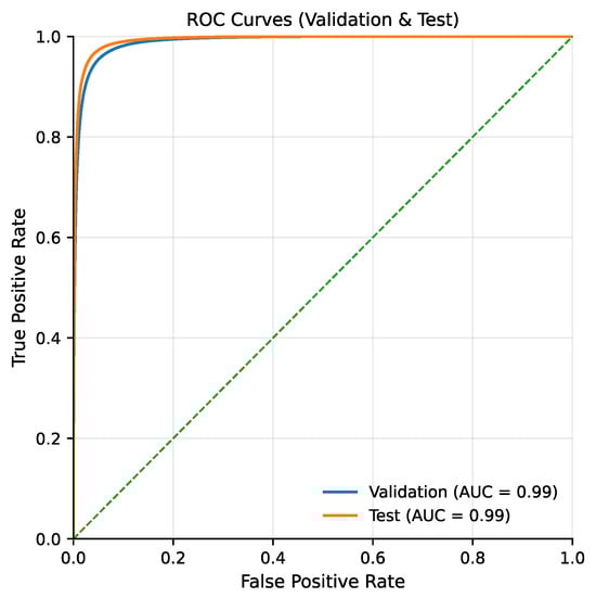
Figure 3. Receiver Operating Characteristic (ROC) curves. The green dashed line represents the performance of a random classifier.

The precision–recall curve (Figure 4) shows that precision remains close to 1.0 across almost the entire recall range, resulting in an Average Precision (AP) of approximately 0.99. This indicates that the model produces very few false positive predictions even when recall is increased, which is critical in temporal communication networks, where incorrectly predicted links may lead to misleading conclusions about future interaction patterns. The observed stability of precision highlights the suitability of the proposed model for ranking-based link prediction tasks.

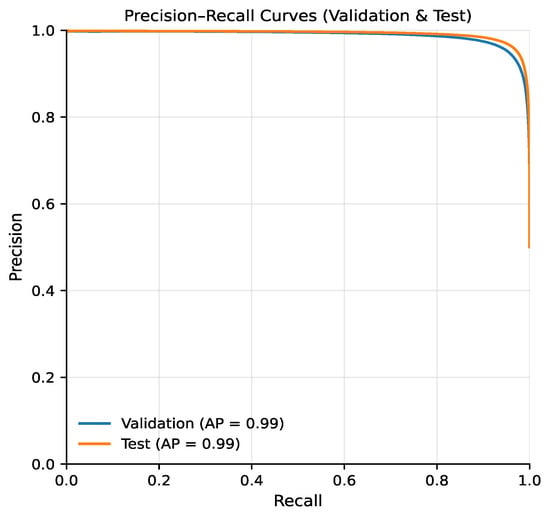
Figure 4. Precision-Recall curves for validation and test sets.

The score distributions for positive and negative edges (Figure 5) reveal a clear separation between the two classes, with positive links receiving scores concentrated near 1 and negative links near 0. The optimal F1 threshold selected on the validation set (approximately 0.589) lies within a low-density region between these distributions, providing a natural margin for decision-making. This separation reduces sensitivity to small threshold variations and contributes to stable classification behavior in dynamic graph settings.

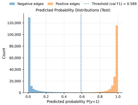
Figure 5. Score distributions.

The calibration curve (Figure 6) remains close to the diagonal in the higher predicted probability ranges, indicating good agreement between predicted confidence levels and observed link frequencies in regions where the model is most certain. A slight under-confidence is visible in mid-range probability bins; however, this effect does not substantially impact performance, as the majority of high-confidence predictions correspond to true future links. Good calibration is particularly relevant for temporal link prediction scenarios where predicted probabilities may be used as inputs to higher-level decision processes.

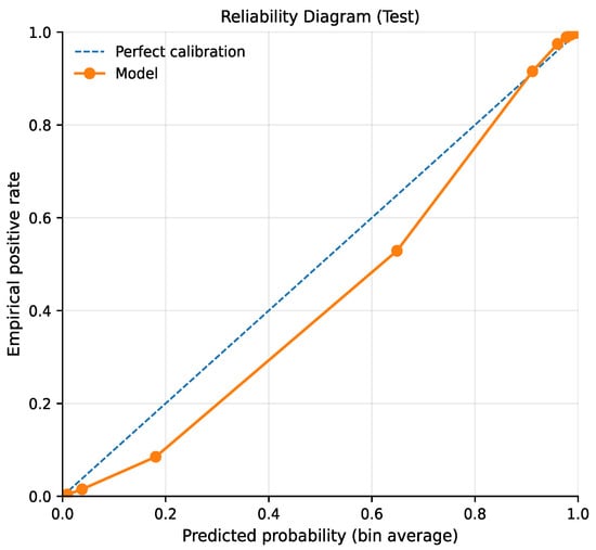
Figure 6. Calibration.

The threshold analysis (Figure 7) demonstrates that around the validation-selected threshold (approximately 0.589), the model achieves a balanced trade-off between precision and recall, resulting in an F1 score of approximately 0.96. Within this narrow region, both metrics remain high and stable, indicating a well-defined operating point. Moving the threshold away from this region causes a rapid degradation of either precision or recall, highlighting the importance of validation-based threshold selection in temporal link prediction tasks.

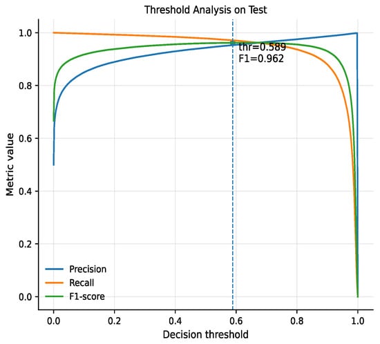
Figure 7. Threshold analysis. The vertical blue dashed line indicates the optimal decision threshold (thr = 0.589) determined by maximizing the F1-score.

The Precision@K curve (Figure 8) shows that precision remains close to 1.0 for small values of K and decreases gradually as K increases. This behavior indicates that the highest-ranked predictions are predominantly true positive edges, confirming that the model effectively orders potential links by their likelihood of future occurrence. Such ranking quality is particularly valuable in practical scenarios where only a limited number of top predictions can be acted upon.

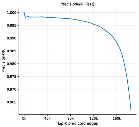
Figure 8. Precision-K test.

The cumulative gain curve (Figure 9) closely follows the ideal reference line, reaching a large fraction of positive instances after selecting only a relatively small subset of the highest-ranked edges. This demonstrates that the proposed model efficiently prioritizes true future links, allowing effective identification of emerging interactions with minimal inspection effort. This property is crucial for large-scale temporal networks where exhaustive evaluation of all candidate links is infeasible.

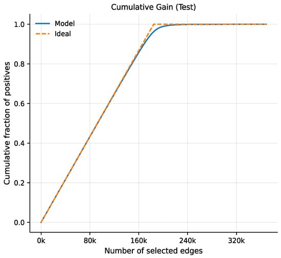
Figure 9. Cumulative gain test.

Figure 10 presents the confusion matrix in terms of absolute counts. The number of true positive and true negative predictions substantially exceeds the number of false positives and false negatives, indicating that the majority of link existence decisions are correct under the selected operating threshold. The relatively small error mass suggests that misclassifications constitute only a minor fraction of all evaluated node pairs. From the perspective of temporal link prediction, this result confirms that the proposed model successfully captures the dominant interaction patterns driving future email exchanges while limiting spurious link predictions that could distort the interpretation of network dynamics.

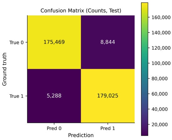
Figure 10. Confusion matrix counts for the test set. The color scale indicates the density of predictions, where lighter colors (yellow) represent higher values and darker colors (purple) represent lower values.

Figure 11 shows the normalized confusion matrix, highlighting class-wise performance independent of class imbalance. The recall for the positive class is approximately 0.97, indicating that most future links are correctly identified, while the specificity for the negative class is around 0.95, reflecting a low false-positive rate for non-existing connections. This balanced behavior across classes demonstrates that the classifier does not overly favor either link emergence or non-emergence. Such stability is particularly important in temporal communication networks, where class proportions may vary significantly across time windows and datasets.

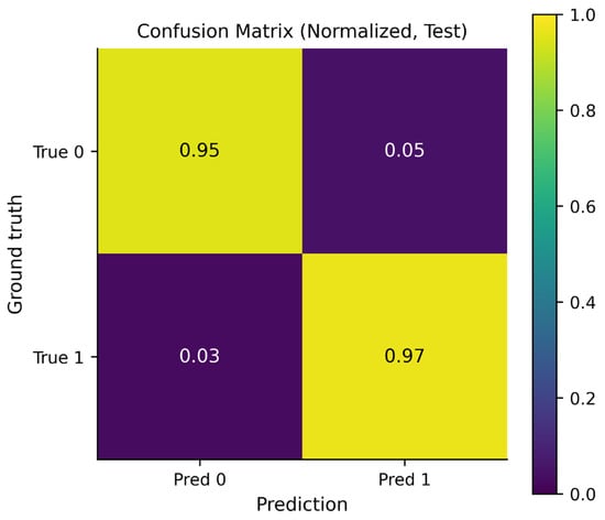
Figure 11. Normalized confusion matrix for the test set. The color intensity represents the proportion of predictions, where lighter colors (yellow) indicate higher values (closer to 1.0) and darker colors (purple) indicate lower values.

6. Discussion

In our experiments, we analyzed the topology of numerous technology-based networks, with the results proving that traditional (structural) link prediction methods often return unsatisfactory results when processing temporal networks built from data divided into short time windows. On the other hand, the dynamic complex network shows statistically stable patterns of local connections, despite the fact that stability of a single link is quite low. This leads to the conclusion that methods based on time series analysis and learning should lead to better results, which was confirmed with the application of the TGNN model proposed in this article, which returned good results when applied to sparse networks analyzed in short timescales. The promising results of these experiments open possibilities for further development. The most appealing directions are as follows:

• Including link weight in the analysis: In an email network, a link exists as a consequence of sending one or many messages, and in most cases, it is far more stable in the second case. This issue could be used to improve our method, and also to test it with longer time windows, within which intensity of communication could be clearly distinguished.
• Incorporating group detection and group evolution in learning models, which could allow learning typical node interaction patterns within clusters of nodes (network communities).

7. Conclusions

The results prove that our model adequately learns about changing email communication patterns, showing results that exceed those achieved by similar approaches. It must be noted, however, that it is sometimes difficult to compare experimental results within the area of link prediction using neural networks—there are differences on the level of graph scale and data preparation, as well as in the inherent dynamics of the analyzed graph itself. In the case of the WUST email network, we used data covering almost two years of operation. Dividing the data into relatively small frames (1, 3, and 7 days) allowed us to properly train the model, positively impacting its accuracy. This could not be achieved when working with only a few network snapshots (time windows). Moreover, the graphs built from 1-day email log data tend to be more sparse, making to possible to learn precisely about ongoing patterns of activity (email exchanges). In sum, the high precision at the best threshold shows that the model can reliably predict future communication links based on past communication logs, with a low number of false positive results.

References

- Kleinberg, J. The convergence of social and technological networks. Commun. ACM 2008, 51, 66–72. [Google Scholar] [CrossRef]
- Barabási, A.-L. The origin of bursts and heavy tails in humans dynamics. Nature 2005, 435, 207. [Google Scholar] [CrossRef] [PubMed]
- Braha, D.; Bar-Yam, Y. From Centrality to Temporary Fame: Dynamic Centrality in Complex Networks. Complexity 2006, 12, 59–63. [Google Scholar] [CrossRef]
- Kempe, D.; Kleinberg, J.; Kumar, A. Connectivity and inference problems for temporal networks. J. Comput. Syst. Sci. 2002, 64, 820–842. [Google Scholar] [CrossRef]
- Lahiri, M.; Berger-Wolf, T.Y. Mining Periodic Behavior in Dynamic Social Networks. In Proceedings of the 2008 Eighth IEEE International Conference on Data Mining (ICDM), Pisa, Italy, 15–19 December 2008; pp. 373–382. [Google Scholar]
- Singh, L.; Getoor, L. Increasing the Predictive Power of Affiliation Networks. IEEE Data Eng. Bull. (DEBU) 2007, 30, 41–50. [Google Scholar]
- Lieben-Nowell, D.; Kleinberg, J.M. The link-prediction problem for social networks. J. Am. Soc. Inf. Sci. Technol. 2007, 58, 1019–1031. [Google Scholar] [CrossRef]
- Bai, Q.; Nie, C.; Zhang, H.; Zhao, D.; Yuan, X. Hgwavenet: A hyperbolic graph neural network for temporal link prediction. In Proceedings of the ACM Web Conference 2023, Austin, TX, USA, 30 April–4 May 2023; pp. 523–532. [Google Scholar]
- Abbas, K.; Abbasi, A.; Dong, S.; Niu, L.; Chen, L.; Chen, B. A Novel Temporal Network-Embedding Algorithm for Link Prediction in Dynamic Networks. Entropy 2023, 25, 257. [Google Scholar] [CrossRef]
- Manuel Dileo, M.; Gaito, Z. Temporal graph learning for dynamic link prediction with text in online social networks. Mach. Learn. 2024, 113, 2207–2226. [Google Scholar] [CrossRef]
- Jin, R.; Liu, X.; Murata, T. Predicting popularity trend in social media networks with multi-layer temporal graph neural networks. Complex Intell. Syst. 2024, 10, 4713–4729. [Google Scholar] [CrossRef]
- Getoor, L.; Diehl, C.P. Link mining: A survey. ACM SIGKDD Explor. Newsl. 2005, 7, 3–12. [Google Scholar] [CrossRef]
- Huang, Z.; Lin, D.K.J. The Time-Series Link Prediction Problem with Applications in Communication Surveillance. Inf. J. Comput. 2009, 21, 286–303. [Google Scholar] [CrossRef]
- Liu, Y.; Wu, D.; Liang, Y. Survey on Graph-Based Reinforcement Learning for Networked Coordination and Control. Automation 2025, 6, 65. [Google Scholar] [CrossRef]
- Leskovec, J.; Krevl, A. Email-Eu-Core Temporal Network; Stanford Network Analysis Project (SNAP): Stanford, CA, USA, 2014. [Google Scholar]
- Leskovec, J.; Krevl, A. CollegeMsg; Stanford Network Analysis Project (SNAP): Stanford, CA, USA, 2014. [Google Scholar]
- Kipf, T.N.; Welling, M. Semi-Supervised Classification with Graph Convolutional Networks. In Proceedings of the International Conference on Learning Representations (ICLR), Toulon, France, 24–26 April 2017. [Google Scholar]
- Gilmer, J.; Schoenholz, S.S.; Riley, P.F.; Vinyals, O.; Dahl, G.E. Neural Message Passing for Quantum Chemistry. In Proceedings of the 34th International Conference on Machine Learning (ICML), Sydney, Australia, 6–11 August 2017; pp. 1263–1272. [Google Scholar]
- Hamilton, W.L.; Ying, R.; Leskovec, J. Inductive representation learning on large graphs. arXiv 2017, arXiv:1706.02216. [Google Scholar] [CrossRef]
- Paszke, A.; Gross, S.; Massa, F.; Lerer, A.; Bradbury, J.; Chanan, G.; Killeen, T.; Lin, Z.; Gimelshein, N.; Antiga, L.; et al. PyTorch: An imperative style, high-performance deep learning library. Adv. Neural Inf. Process. Syst. 2019, 32, 8024–8035. [Google Scholar]
- Fey, M.; Lenssen, J.E. Fast graph representation learning with PyTorch Geometric. arXiv 2019, arXiv:1903.02428. [Google Scholar] [CrossRef]
- Pedregosa, F.; Varoquaux, G.; Gramfort, A.; Michel, V.; Thirion, B.; Grisel, O.; Blondel, M.; Prettenhofer, P.; Weiss, R.; Dubourg, V.; et al. Scikit-learn: Machine learning in Python. J. Mach. Learn. Res. 2011, 12, 2825–2830. [Google Scholar]
- Hagberg, A.; Schult, D.; Swart, P. Exploring network structure, dynamics, and function using NetworkX. In Proceedings of the 7th Python in Science Conference (SciPy2008), Pasadena, CA, USA, 19–24 August 2008; Varoquaux, G., Vaught, T., Millman, J., Eds.; SciPy Proceedings Organization: Pasadena, CA, USA, 2008; pp. 11–15. [Google Scholar]
- Leskovec, J.; Krevl, A. SNAP Datasets: Stanford Large Network Dataset Collection; Stanford Network Analysis Project (SNAP): Stanford, CA, USA, 2014. [Google Scholar]
- Paranjape, A.; Benson, A.R.; Leskovec, J. Motifs in Temporal Networks. In Proceedings of the 10th ACM International Conference on Web Search and Data Mining (WSDM), Cambridge, UK, 6–10 February 2017; pp. 601–610. [Google Scholar]
- Juszczyszyn, K.; Musiał, K.; Kazienko, P. Local Topology of Social Network Based on Motif Analysis. In Proceedings of the 12th international conference on Knowledge-Based Intelligent Information and Engineering Systems, KES 2008, Zagreb, Croatia, 3–5 September 2008; LNAI; Springer: Berlin/Heidelberg, Germany, 2008. [Google Scholar]
- Juszczyszyn, K.; Budka, M.; Musiał, K. Link prediction based on subgraph evolution in dynamic social networks. In Proceedings of the IEEE International Conference on Social Computing, PASSAT/SocialCom, Boston, MA, USA, 9–11 October 2011; IEEE Computer Society: Boston, MA, USA, 2011; pp. 27–34. [Google Scholar][Green Version]
- Kazemi, S.M.; Goel, R.; Jain, K.; Kobyzev, I.; Sethi, A.; Forsyth, P.; Poupart, P. Representation Learning for Dynamic Graphs: A Survey. J. Mach. Learn. Res. 2020, 21, 2648–2720. [Google Scholar]
- Rossi, E.; Chamberlain, B.; Frasca, F.; Eynard, D.; Monti, F.; Bronstein, M. Temporal Graph Networks for Deep Learning on Dynamic Graphs. arXiv 2020, arXiv:2006.10637. [Google Scholar] [CrossRef]
- Kipf, T.N.; Welling, M. Variational graph auto-encoders. arXiv 2016, arXiv:1611.07308. [Google Scholar] [CrossRef]
Disclaimer/Publisher’s Note: The statements, opinions and data contained in all publications are solely those of the individual author(s) and contributor(s) and not of MDPI and/or the editor(s). MDPI and/or the editor(s) disclaim responsibility for any injury to people or property resulting from any ideas, methods, instructions or products referred to in the content. |
© 2026 by the authors. Licensee MDPI, Basel, Switzerland. This article is an open access article distributed under the terms and conditions of the Creative Commons Attribution (CC BY) license.