Cross-Course Knowledge Tracing for Student Performance Prediction in MOOCs

Abstract

Knowledge tracing (KT), which uses machine learning models to predict students’ future performance, has received a lot of attention in intelligence education. However, in Massive Open Online Courses (MOOCs), most of the existing KT methods can only track students’ performance in one course. In addition, when there is scant learning record data on new courses, training a new KT model becomes challenging. Furthermore, existing KT methods tend to excel in specific courses, but their generalization ability is inferior when faced with similar or distinct courses. To address these challenges, this paper proposes a MOOC-oriented cross-course knowledge tracing model (MCKT). In MCKT, we first construct two attribute relationship graphs to obtain the student and KC representations from the source course and the target course, respectively. Then, the element-wise attention mechanism is used to fuse the student representations from both courses. Next, MLPs are used to reconstruct the interaction between students and KCs in each course to enhance students’ cross-course representation. Finally, recurrent neural networks (RNNs) are used to predict the students’ performance in each course. Experiments show that our proposed approach outperforms existing KT methods in predicting students’ performance across diverse MOOCs, proving its effectiveness and superiority.

1. Introduction

The fourth industrial revolution, driven by the integration of intelligent technologies such as the Internet of Things (IoT), big data analytics, and Artificial Intelligence (AI), has transformed the way data is generated and decisions are made in both industrial and societal domains. Machine learning architectures like Transformers have become essential for automating complex analytical tasks. In industrial settings, these models learn from sensor data and operational logs to carry out tasks such as predictive maintenance and quality control. On social media and digital platforms, they process vast amounts of sequential and graph-structured interaction data to drive content recommendations and user behavior modeling. This also provides important analogies and a technical foundation for the field of education, enabling the emergence of knowledge tracing (KT) models. KT models can help intelligent tutoring systems dynamically understand the students’ mastery of knowledge, make timely adjustments to the teaching plans, and recommend relevant teaching resources for students. To study this issue in depth, many efforts have been made to devise various methods of KT. One of the most widely used is deep knowledge tracing (DKT) [1] based on the deep learning method. DKT typically employs long short-term memory networks (LSTMs) to model students’ learning interaction state. DKT converts students’ exercise-answering performance history into a time series to predict students’ answers in the next step and infer their mastery of KCs. On this basis, many deep learning-based KT models, such as CNN-KT [2], Transformer-KT [3], and GNN-KT [4], have also been proposed to improve KT models’ performance.

Although these KT models have proven to be effective, it is still difficult to play to their strengths in Massive Open Online Course (MOOC) scenarios. (i) Single-Course Limitation: The traditional KT models only track the knowledge mastery status of students in a certain course and cannot predict their performance in another course. However, MOOCs include a large number of courses, and it is common in practice for a student to study more than one course at the same time. Figure 1 show four students in course a and four students in course b, where $Kate$ and $Tom$ are enrolled in both courses (referred to as common students in this study). Students learn different KCs in different courses, but most existing KT models cannot capture the performance of a student in different courses.

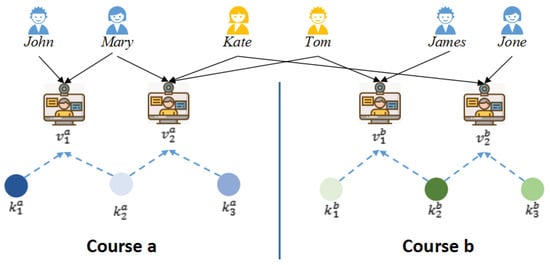
Figure 1. Schematic diagram of MOOC user learning.

(ii) Data Scarcity Issue: There is a common problem of scarcity of learning record data in MOOCs [5], which will lead to difficulty in training the KT model of a single course. KT methods rely on large amounts of historical data from students to build models and make accurate predictions. Yet, in MOOCs, especially in newly opened courses or in the educational setting of some schools, learning record data may be very limited or non-existent, making it difficult to apply training KT. (iii) Generalization Difficulty: A course in the MOOCs usually has a long learning cycle and requires students to continuously invest time. As a result, students often want to predict how they will perform on a new course before they start that course in order to make better decisions about whether to start learning or how to plan for it. Nevertheless, the existing KT models only focus on one course, lack generalization ability, and cannot be used to predict the performance of students in the new course. (iv) Lack of Video Interaction Mapping: In addition, most of the courses in MOOCs contain many instructional videos, and the task of answering questions after watching the videos is not mandatory. However, most of the existing KT models map the level of mastery of KCs based on the results of students answering exercises. Due to the lack of a method to map the mastery level of KCs according to students’ video browsing behavior, the existing KT models cannot be widely used in MOOCs. These limitations hinder the realization of robust, automated learner modeling in MOOCs—a context characterized by massive scale and data-rich interactions where such technology should offer significant value.

To overcome these hurdles and advance towards truly adaptive MOOC platforms, we propose a transfer learning-based MOOC cross-course knowledge tracing method, namely MCKT, to predict students’ learning performance in the next step of a different course. The framework of MCKT can be divided into three parts, i.e., data pre-processing, pre-training, and prediction. In the part of data pre-processing, we extract the sequence of students’ interaction with knowledge concepts (KCs) based on the interaction records between students and items (e.g., exercises and videos) in the MOOC dataset; this approach follows the classic way of dealing with knowledge tracing datasets. In the part of pre-training, two graph structures are used: (i) we use the skip-gram algorithm to obtain the initial student representation in the structure of the attribute relationship graph (ARG); (ii) we use element-wise attention and a multi-layer perception (MLP) to reconstruct the interaction relationship between the students and KCs in the Interaction Relationship Graph (IRG) structure after the cross-course method. By using the above two graph structures in the pre-training, the students’ representations not only combine the similarity of students’ attributes in the source course and the target course, but also combine their relationship with KCs in the source course. In the prediction phase, the RNNs are used to model the results of the interaction between students and KCs and predict students’ mastery of the next KC in both the source and target courses.

In summary, the contributions of this study are threefold:

• This paper proposes a MOOC-oriented cross-course KT method based on transfer learning, which predicts the status of the next stage of students’ learning in the different MOOCs with unbalanced learning records.
• This paper proposes a method to evaluate the mastery of KCs by using the information of video viewing in MOOCs so that the KT model can be applied to video viewing behavior, not only to answer exercises.
• This paper reports on the extensive experiments that were conducted in six scenarios based on two real MOOC datasets. The experiments verify that the proposed model is more effective than the existing KT methods in cross-course KT tasks.

The rest of this paper is organized as follows. Section 2 briefly reviews the related work. Section 3 introduce the problem statement. Section 4 describes the framework and the implementation of the proposed approach in detail. Extensive experimental studies to validate the effectiveness of our model and several research questions are addressed in Section 5. Section 6 concludes this work, analyzes this study’s limitations, and proposes future research directions.

2. Related Work

2.1. Knowledge Tracing

The term knowledge tracing was introduced by [6]. In a study period, the teacher can estimate the probability of the students mastering each KC. Based on the estimated probability, the teacher can propose a personalized sequence of exercises to students until they master all the KCs. In the original KT model, the probability estimation of students’ learning performance adopted the Bayesian probability formula, called Bayesian Knowledge Tracing (BKT). Lin et al. proposed the intervention-BKT model by adding intervention nodes to the original BKT model [7]. In [1], Piech et al. proposed a knowledge tracing model based on RNNs, named deep knowledge tracing (DKT). Using records of the exercises answered, the model learns to predict the probability that a student can correctly answer subsequent exercises. DKT adopts LSTM, a variant of RNNs, to perform prediction tasks, as LSTM has a good effect on sequence-based prediction. The advantage of the DKT model has been verified on other datasets, in classic programming courses [8], and in courses studied by watching videos [9]. DKT summarizes a student’s mastery level of all concepts by one hidden state, making it difficult to trace to what degree a student has mastered a certain concept. To address this issue, Zhang et al. proposed dynamic key–value memory networks (DKVMNs), which can accurately indicate the mastery state of each concept [10]. The DKVMN initializes a static matrix called key, which stores the concepts, and a dynamic matrix called value, which stores and updates the corresponding concepts’ mastery through reading and writing operations. In order to improve the interpretability, a Markov blanket-based KT model was proposed by [11], which applied interpretable machine learning techniques in a KT task.

2.2. Cross-Domain Prediction

In the field of cross-domain prediction, researchers have proposed a series of methods to solve the transfer learning problem between different domains. The existing cross-domain prediction algorithms can be divided into three categories according to the different deep transfer learning techniques: (i) Cross-domain prediction algorithms based on feature mapping can align features between the source and target domains, thereby enabling the transfer of knowledge from the source to the target domain. In this process, attention-based mechanisms are often employed to capture complex relationships among data [12]. (ii) Cross-domain prediction algorithms based on instance transfer improve the existing results or models in the transfer learning pre-trained network as a whole and weight the features of different domains to break the data sparsity effect of cross-domain prediction. (iii) The third category is cross-domain prediction algorithms based on adversarial transfer based on generative adversarial networks (GANs). This method is integrated into the cross-domain prediction problem to solve the feature domain adaptation problem. Cross-domain prediction technology has applications in various fields, such as medical services, network security, and semantic feature processing. However, in the field of education data mining, the research in cross-course personalized learning recommendation is still in its early stage. Although some progress has been made in cross-domain prediction, most existing methods only focus on transfer learning between discrete domains, ignoring transfer learning between continuous-time domains.

Recently, researchers have begun to focus on how to use the knowledge gained in one subject area by transfer learning to complement and improve the learning process in other areas. To solve the problems of domain-specific limitations and data sparsity in the current KT methods [13]. Cheng et al. proposed a three-step adaptive KT model [14], which introduced the maximum mean discrepancy (MMD), where the difference in data distribution between different domains is narrowed to achieve the effective use of knowledge between domains. However, MMD is sensitive to parameters and requires a large amount of target domain data for effective domain adaptation, and the adaptability of the model may be limited if the target domain data is extremely scarce [15]. To solve the problem of knowledge distribution bias between different courses, Huang et al. proposed a STAN framework [16], which aligned the difficulty distribution of the two domains using conditional adversarial learning and difficulty-based sampling methods. However, the embedding mechanism of these methods mainly relies on serialized coding and fails to consider the graph topology information implied by the course KCs or common students as middle-layer embeddings.

3. Problem Statement

In this section, we first review the definition of knowledge tracing. Then, we introduce the graph structure used to represent the relationships between the students and items in the MOOC. Finally, we explain the cross-course knowledge tracing in MOOC scenarios. Some important notations are listed in Table 1, and we present a more detailed explanation of their role in the context.

Table 1. Some important notations.

Notation	Description
$C^a$, $C^b$	Course a and b in a MOOC platform.
$s\in S$, $\left|S\right|$	The students in a MOOC platform and the number of students.
$v\in V$, $\left|V\right|$	The items in a MOOC platform and the number of items.
$k\in K$, $\left|K\right|$	The KCs in a MOOC platform and the number of KCs.
$\alpha$	The result of the interactions.
$(v_{t_0},{\alpha }_{t_0})\in I$	The record sequence of students interacting with the items.

Knowledge Tracing. Given the sequence of students’ learning interactions in online learning systems, knowledge tracing aims to monitor students’ changing knowledge states during the learning process and accurately predict their performance on the next items. Formally, in an intelligent education system, suppose the number of students, items, and KCs are denoted as $\left|S\right|$, $\left|V\right|$, and $\left|K\right|$, respectively. For a student $s\in S$, the sequence of items (e.g., video or exercise) with which the student interacted is recorded, denoted as $I=\{(v_{t_0},{\alpha }_{t_0}),\dots ,(v_{t_i},{\alpha }_{t_i}),\dots \}$, where $v_{t_i}\in V$ is the item that appeared at time step $t_i$ and ${\alpha }_{t_i}$ indicates the corresponding score. For instance, if the answer of the exercise is correct, ${\alpha }_{t_i}$ is 1 (or tick); otherwise, ${\alpha }_{t_i}$ is 0 (or cross). Knowledge tracing can be formulated as follows:

$$P{r}_s({\alpha }_{t_{n+1}}=1)=\Omega \left(v_{t_{n+1}}\right|I_{t_n}^s,V_{t_n}),$$

(1)

where, $P{r}_s$ denotes the probability of correctly answering. Interaction Relationship Graph. In the process of viewing videos or answering exercises during the course learning, there are heterogeneous relationships among students, items, and KCs [17,18]. An Interaction Relationship Graph (IRG) is denoted as $G=\{\mathbb{V};\mathbb{E}\}$, consisting of an object set $\mathbb{V}$ and a link set $\mathbb{E}$. $\mathbb{V}$ is a set of object types (e.g., student, item, or KC). $\mathbb{E}$ is a set of relation types, and $\mathbb{E}=\{r_A,r_C\}$, where $r_A$ represents the relation interact and $r_C$ represents the relation contains.

As shown in Figure 1, for the IRG of course a, $Mary$ views the video $v_1^a$ and $v_2^a$. $v_2^a$ requires KCs $k_2^a$ and $k_3^a$. $v_1^a$ requires KC $k_1^a$. From the figure, we can observe that there is a relationship between $k_2^a$ and $k_3^a$ through $v_2^a$, and there is also a relationship between $v_1^a$ and $v_2^a$ through $Mary$. The reason is that $Mary$ views both videos during her learning process. In the KT task, the prediction of KC mastery is more general, so in this work, the IRG is used to model the relationship between students and KCs in a MOOC.

Cross-Course Knowledge Tracing. Students often enroll in more than one course in MOOCs. As shown in Figure 1, suppose there are two courses a and b, denoted by $C^a=(S_{com}^a,S_{dis}^a,V^a,I^a)$ and $C^b=(S_{com}^b,S_{dis}^b,V^b,I^b)$, where $S_{com}^a$ and $S_{com}^b$ represent students who have taken both course a and course b (i.e., Kate and Tom, referred to as ‘common students’). $S_{dis}^a$ represents the distinct students in course a (i.e., John and Mary), and $S_{dis}^b$ represents the distinct students in course b (i.e., James and Jone). Students enrolled in different courses are referred to as ‘distinct students’ in this paper. $V^a$ and $V^b$ represent the set of items of $C^a$ and $C^b$ separately. I signifies the set of interactions. Given the respective interaction records in these two courses, the goal of the cross-course knowledge tracing is to predict students’ mastery level of knowledge in b/a courses using the interaction data observed by a student in the a/b course.

Given a sequence of learning resources items $V_{t_n}^a=\{v_{t_1},v_{t_2},\dots ,v_{t_n}\}$ of the course a, if student s has learned on $V_{t_n}^a$, and the interaction recording is denoted by $I_{t_n}^s$, then the probability of the knowledge mastery of this student on the course b is calculated as

$$P{r}_s({\alpha }_{t_{n+1}}^b=1)=\Omega \left(v_{t_{n+1}}^b\right|I_{t_n}^s,V_{t_n}^a),$$

(2)

where $Pr({\alpha }_{t_{n+1}}^b=1)$ represents the probability of answering correctly, which usually also reflects the mastery level of student s on the corresponding KC of the course b at the next time step, and the closer its value is to 1, the higher the student’s mastery level.

4. Proposed Approach

To address the problem introduced in Section 1, this paper proposes a novel KT method for cross-course student performance prediction in MOOCs, namely MCKT. As shown in Figure 2, the framework of MCKT is divided into the three modules, i.e., the Course graph construction module, the Cross-course embedding combination module , and the Knowledge performance prediction module. At the beginning, we extract data from the MOOC dataset that can be used for cross-course KT, including students, items, the text of KCs, the KCs contained in the items, and the results of students’ interaction with the items. Then, we calculate the similarity of the textual information of students, projects, and KCs in two courses (e.g., $C^a$ and $C^b$) to form an attribute relationship graph (ARG). Next, an attention mechanism and the MLP are employed in the Cross-course embedding combination module to generate the cross-course fusion representations of the common students, which is combined with the features from courses a and b. Finally, all students’ representations and the interaction results are sent to the Knowledge performance prediction module to predict students’ performance.

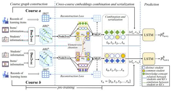
Figure 2. The framework of MCKT taking course a and course b as examples. The $ARG$ and $IRG$ are constructed by pre-processing the dataset, and the representations of the students and KCs are obtained. Then the representations of the cross-course common students and distinct students are obtained by pre-training. Next, the cross-course representations of the students and KCs from time $t_0$ to $t_n$ are input into the prediction layer to predict the knowledge state at the $t_{n+1}$ step.

4.1. Data Pre-Processing

In reality, some MOOC platforms provide exercises or tasks containing KCs for the courses, such as MOOPer, which has many online exercises for each course. However, to increase utilization [5], some MOOC platforms provide learning videos that contain KCs, such as MOOC-Cube, and do not necessarily provide online exercises for all courses, nor do they force students to answer online exercises. Video-watching sequences (e.g., play, pause, fast-forward, and replay) exhibit temporal patterns that have been shown in prior research [19,20] to correlate with learning attention and self-regulation (e.g., studies on clickstream analysis for engagement inference). Therefore, converting these sequences into simulated knowledge states provides a plausible, data-driven approximation. Based on this assumption, for courses that provide only video-watching logs but no exercise response records, we follow the method described in Reference [9], which uses the processed video-watching log data as the input data.

The first step involves consolidating information from the students watching the video. The initial representation of a student is constructed from five kinds of data, i.e., the learned courses C; the learned videos V; the number of times a student watched a learned video m; the duration of each learned video l; and the average duration that the s-th student spent on each learned video $\tau$. We consider that the student’s mastery level of each KC is determined by the ratio of the average duration of the corresponding video learned by them to the total duration of the video. The process of obtaining the result of the interaction is formalized as

$${\alpha }^v=tanh({\displaystyle \frac{{\tau }^v}{l^v}}\times m^v),$$

(3)

where ${\alpha }^v$ represents the result of the student’s interaction with video v.

In the second step, the student’s ID, the learned video’s ID, and the mastery probability of the KC in the learned video (each video contains one KC) are combined into a triplet I to form a sequence of the student’s interaction–response to the video:

$$I_t=(s,v_t,{\alpha }_t^v),$$

(4)

where $I_t$ represents an interaction between the student and video v at time t.

The third step is to generate two specific representations of each student. One reflects the student’s association with the learning videos (or other items, such as exercises), denoted by $E\left(g\right)$,

$$E{\left(g\right)}_{t_n}=\{{(s_1,v_1,k_1)}_{t_1},{(s_2,v_2,k_2)}_{t_2},\dots ,{(s_i,v_j,k_m)}_{t_n}\},$$

(5)

where $E\left(g\right)$ is the initial data for the IRG, which is used to further generate cross-course representations in the Cross-course embedding combination module. And the other reflects the KCs and state time series of the learning interaction, which is denoted by $E\left(x\right)$,

$$E{\left(x\right)}_{t_n}=\{I_{t_1},I_{t_2},\dots ,I_{t_n}\},$$

(6)

where $E\left(x\right)$ is employed to further model the student’s mastery of KCs in the Knowledge performance prediction module.

4.2. Course Graph Construction

In this module, a weighted attribute relationship graph (ARG) for each course is formed. $E\left(g\right)$ is input to this module. The similarity of the text representation vectors is calculated to generate edge weights between corresponding nodes. The text representations of students and KCs are derived using Doc2Vec [21] from their respective textual attributes: student ID, name, and enrolled courses for students and KC ID and textual description for knowledge components. The pairwise similarities among these resulting embedding vectors are then used to construct the weighted edges of the ARG connecting students to students, students to KCs, and KCs to KCs. The text representations’ similarities are formalized as the following Equations (7)–(9).

$$\omega (s,k)={\mathbf{W}}_{sk}\times \theta (s,k),$$

(7)

$$\omega (s,s)={\mathbf{W}}_{ss}\times \theta (s_i,s_j),$$

(8)

$$\omega (k,k)={\mathbf{W}}_{kk}\times \theta (k_i,k_j),$$

(9)

where s denotes the student node, k represents the KC node, ${\mathbf{W}}_{sk},{\mathbf{W}}_{ss},{\mathbf{W}}_{kk}\in {\mathbb{R}}^{d\times V}$ are the constant coefficient matrices, and $\omega (·)$ represents the relationship weight between nodes. $\theta (·)$ represents the cosine similarity. Through the above steps, a weighted ARG is created for each course.

Then, the Node2vec [22] module is employed to generate the node embeddings of these two ARGs. The embedding of a node is denoted by $\hat{x}$. The Node2vec module adopts the principle of similarity of adjacent nodes, uses the central node to predict the context node, and obtains the embedding of the target node after continuous iterative optimization. Node2Vec uses the skip-gram model to learn the embedding representation of the node. The goal of the skip-gram model is to predict the node itself based on its context. The optimization objective of Node2vec is

$${\mathcal{L}}_{node2vec}=\underset{f}{max}\sum _{u\in V}[-log{Z}_u+\sum _{n_i\in N_S\left(u\right)}f\left(n_i\right)·f\left(u\right)],$$

(10)

where f is a function that maps each node u to a d-dimensional space vector, e.g., $f=V\to R^d$. u is the current node, $n_i$ is the neighbor node of the u node obtained through the paths of the ARGs, and $Z_u={\sum }_{v\in V}exp\left(f\right(u)·f(v\left)\right)$. Stochastic gradient descent is used to optimize ${\mathcal{L}}_{node2vec}$.

4.3. Cross-Course Embedding Combination

Considering that students are the subjects of cross-course learning behaviors and the importance of users in information systems [23], we propose to leverage the representation of students who have taken both the source and target courses as a transferable ’bridge’. Specifically, these overlapping students’ behavioral patterns in both courses are modeled and fused to establish a shared latent space, enabling knowledge transfer for new students in the target course based on their similarity to these bridge students in the source course. The representation of students in two different courses (take course a and course b as examples) are the embeddings of the student nodes in two ARGs. The task of this module is to generate the cross-course representations of students shared by course a and course b. In this module, the comment students’ representations are generated through element-wise attention [24]. Consequently, it attains high expressivity with neuron-level degrees of freedom [25]. We denote the representations of student $s_i$ in course a by $E\left(C^a\right|s_i)$; we denote the representations of student $s_j$ in course b by $E\left(C^b\right|s_j)$. The process of cross-course feature combination is shown in the middle part of Figure 2.

The cross-course representations of students must be further processed before sequence modeling can be performed. The element-wise attention mechanism combines the common students’ embedding representations in courses a and b, and then a matrix multiplication calculation is performed on these cross-course representations. Specifically, the representation of common students in courses a and b can be expressed as follows:

$$\tilde{E}\left(C^a\right|s_i)={\mathbf{W}}^{\mathbf{a}}\odot E\left(C^a\right|s_i)+(1-{\mathbf{W}}^{\mathbf{a}})\odot E\left(C^b\right|s_i),$$

(11)

$$\tilde{E}\left(C^b\right|s_j)={\mathbf{W}}^{\mathbf{b}}\odot E\left(C^b\right|s_j)+(1-{\mathbf{W}}^{\mathbf{b}})\odot E\left(C^a\right|s_j),$$

(12)

where ⊙ indicates element multiplication and ${\mathbf{W}}^{\mathbf{a}}$ and ${\mathbf{W}}^{\mathbf{b}}$ are, respectively, the weight matrices of courses a and b in the element-wise attention mechanism. For distinct students and items in different courses, we only keep their embeddings and do not use the attention mechanism because they do not have double embeddings in courses a and b.

We then used two MLPs to reconstruct the non-linear relationship between students and items. We denote the representations of two kinds of students in course a i.e., $[\tilde{E}\left(C^a\right|s_{com}),E\left(C^a\right|s_{dis})]$, by $S^a$ and denote items in course a by $Q^a$. Then, $S^a$ and $Q^a$ are input to the neural node; the result is $h_i^{as}$ and $h_j^{aq}$ following Equations (13)–(16),

$$h_i^{as}=g(S^a\odot W_i^{as}),$$

(13)

$$h_j^{aq}=g(Q^a\odot W_1^{aq}),$$

(14)

$$\widehat{S^a}=g\left({\mathbf{h}}_k^{as}\right)=g(\stackrel{k}{\overbrace{\dots g(g(h_i^{as}\odot W_1^{as}),W_2^{as})}}),$$

(15)

$$\widehat{Q^a}=g\left({\mathbf{h}}_l^{aq}\right)=g(\stackrel{l}{\overbrace{\dots g(g(h_j^{aq}\odot W_1^{aq}),W_2^{aq})}}),$$

(16)

where $g(*)$ is the activation function ReLU and $W_1^{as},W_2^{as},\dots ,W_1^{aq},W_2^{aq},\dots ,\in {\mathbb{R}}^{d\times \left|V\right|}$ are the learnable weights of each layer of the MLP of the student and items, respectively. The label ⊙ denotes element-wise multiplication. We use a cross-entropy loss to reconstruct the relationship between students and items, following Equations (17) and (18):

$$\widehat{y^a}=\sigma (\widehat{S^a}·\widehat{Q^a}),$$

(17)

$$\mathcal{L}(y^a,\widehat{y^a})=y^{a}log(\widehat{y^a})+(1-\widehat{y^a})log(1-y^a),$$

(18)

where $\widehat{y^a}$ is the predicted interaction in course a, $\sigma$ is the activation function sigmoid, and $(·)$ is the inner product. $y^a$ is an observed interaction in course a. By this way, we can also obtain the same kind of loss in course b. The algorithm of the student cross-course representation generation is shown in Algorithm 1.

Algorithm 1 Algorithm of the student cross-course representation generation

Input: The $ARG$s of two courses $AR{G}^a$ and $AR{G}^b$; The weight matrix of the course a and b in the element-wise attention mechanism ${\mathbf{W}}^{\mathbf{a}}$ and ${\mathbf{W}}^{\mathbf{b}}$. ${\theta }_T$ is a termination condition.    Output: Two sets of representations of students used for prediction layer. 1:   for $s^a$ in $C^a$ do 2:    $\{E\left(C^a\right|s_{com}^a),E(C^a|s_{di f}^a)\}\leftarrow \mathrm{skip}-\mathrm{gram}\left(AR{G}^a\right)$. 3:   end for 4:   for $s^b$ in $C^b$ do 5:    $\{E\left(C^b\right|s_{com}^b),E(C^b|s_{di f}^b)\}\leftarrow \mathrm{skip}-\mathrm{gram}\left(AR{G}^b\right)$. 6:   end for 7:   while ${\theta }_T$ not converged do 8:    $E\left(C^b\right|s_{com}^a)\leftarrow \mathrm{Attention}(E\left(C^b\right|s_{com}^b),E\left(C^a\right|s_{com}^a),{\mathbf{W}}^{\mathbf{a}})$ {Equation (11)} 9:    $\{\hat{E}\left(C^b\right|s_{com}^a),\hat{E}(C^a|s_{di f}^a)\}\leftarrow \mathrm{MLP}(E\left(C^b\right|s_{com}^a),E(C^a|s_{di f}^a))$ {Equation (17)} 10:  $E\left(C^a\right|s_{com}^b)\leftarrow \mathrm{Attention}(E\left(C^a\right|s_{com}^a),E\left(C^b\right|s_{com}^b),{\mathbf{W}}^{\mathbf{b}})$ {Equation (12)} 11:  $\{\hat{E}\left(C^a\right|s_{com}^b),\hat{E}(C^b|s_{di f}^b)\}\leftarrow \mathrm{MLP}(E\left(C^a\right|s_{com}^b),E(C^b|s_{di f}^b))$ {Refer to Equation (17) but apply to course b} 12:  end while 13:  return

4.4. Knowledge Performance Prediction

In this module, an LSTM model is utilized to model students’ behavior and response sequences when learning items. Specifically, the cross-domain representations of students and KCs generated by using Algorithm 1 are integrated into $E{\left(x\right)}_{t_n}$ to form the sequence of the learning interaction (e.g., performing exercises or watching videos) and responses containing cross-course information. Here, each student’s learning interaction records and student representations are individually spliced to form the input data. These input data are fed into the LSTM model, which predicts the student’s knowledge state at the next step. The variables are related using a simple network defined by the equations

$${\mathbf{h}}_{t_{n+1}}=tanh({\mathbf{W}}_{hx}E{\left(x\right)}_{t_n}+{\mathbf{W}}_{hh}{\mathbf{h}}_{t_n}+b_h),$$

(19)

$$p_{t_{n+1}}=\sigma ({\mathbf{W}}_{ph}{\mathbf{h}}_{t_{n+1}}+b_p),$$

(20)

where $\sigma$ is the activation function $sigmoid$. ${\mathbf{W}}_{hx}$ is the input weight matrix, ${\mathbf{W}}_{hh}$ is the loop weight matrix, $h_{t_0}$ is the initial state, and ${\mathbf{W}}_{ph}$ is the output weight matrix. $b_h$ and $b_p$ are latent bias and output bias, respectively.

We denote the actual performance of the i-th student on the j-th KC by $r^{ij}$, while the learning interaction results are obtained by Equation (3). We train the model with two strategies based on two types of label values. The first strategy is to treat $r^{ij}$ as a continuous value; i.e.,

$$r_t^{ij}=\left\{\begin{array}{cc}\hfill \Phi \left({\alpha }_{ij}^v\right),& w.r.t\Phi \left({\alpha }_{ij}^v\right)\in (0,1),\\ \hfill null,& otherwise.\end{array}\right.$$

(21)

where $\Phi$ is the normalization operation.

The other is to set $r_{ij}$ to a binary value of 0 or 1; that is,

$$r_t^{ij}=\left\{\begin{array}{cc}\hfill 1,& w.r.t\Phi \left({\alpha }_{ij}^v\right)\ge \theta ,\\ \hfill 0,& w.r.t\Phi \left({\alpha }_{ij}^v\right)<\theta ,\\ \hfill null,& otherwise.\end{array}\right.$$

(22)

where $\theta$ denotes the threshold used to divide the mastery of KCs. The loss functions of these two strategies are both defined as the cross-entropy of the prediction performance p and the real one r; i.e.,

$$\mathcal{L}(r_t^{ij},p_t)=r_t^{ij}log\left(p_t\right)+(1-r_t^{ij})log(1-p_t),$$

(23)

$$\mathbf{L}=\sum _{t=0}^n\mathcal{L}(r_t^{ij},p_t),$$

(24)

Remark: The task of transfer learning is to transfer the model from the source domain to the target domain. However, in our research scenario, a course serves as both the target and source course. In each round of iterative training, we use the two courses in the experiment as source courses for cross-training. In this way, the model we train will consist of two sub-models, each capable of performing two-way cross-domain functions.

5. Experiments

In this section, we first provide detailed information about the dataset and experiment setup. This section then provides details of the extensive experiments that were conducted across six cross-course scenarios and the in-depth analyses. Additionally, to provide a clearer understanding of the model, we address the following key research questions in the subsequent sections:

RQ1: Is MCKT more effective than existing KT models in terms of cross-course knowledge performance prediction or not?

RQ2: What impact do the constituent modules of MCKT have on its performance?

RQ3: How effective is MCKT in predicting similar or non-similar courses?

RQ4: Can MCKT predict a student’s performance in another course?

RQ5: Is there is a difference in the representation of common students and distinct students?

5.1. Overview of Datasets

Our experiments are performed on two classic MOOC platforms that contain multiple courses, i.e., MOOPer [26] and MOOC-Cube [27]. MOOPer extracts the interactive data on users’ participation in practical exercises on the EduCoder platform from 2018 to 2019 and models the attribute information of courses, practices, levels, and KCs and the interrelationships between them in a knowledge graph to construct a large-scale practice-oriented online learning dataset. MOOC-Cube is an open large-scale data repository for natural language processing, knowledge graphs, data mining, and other research areas concerned with massive open online courses. It comprises 706 MOOCs, 38,181 videos, 114,563 KCs, and 199,199 real MOOC users. This data source also contains a large-scale concept graph and related academic papers as additional resources for further utilization. We selected student video interaction data, students’ personal characteristics text, videos, and their corresponding courses’ KCs and KCs’ text. The student video interaction data includes video ID, student ID, the number of times students watch the video, the video duration, and the average length of time students watch the video, and the student’s personal characteristics text encompasses the name of the student, the title of the course, etc.; the KC’s text relates to its name and information summary.

To analyze the effect of the proposed method on courses in the same discipline and interdisciplinary courses, we select part of the course data from MOOPer and MOOC-Cube based on the discipline division to form three experiment datasets.

• Dataset I—All belong to the same discipline
  Course A comes from MOOPer’s course “C/C++ programming”. We randomly selected 20,500 interactive data items for it, including 1224 students and 26 KCs.
  Course B comes from MOOPer’s course “Data Structures & Algorithms (C/C++)”. We randomly selected 55,578 interactive data items for it, including 2925 students and 134 KCs.
  Course C comes from MOOPer’s course “Introduction to Artificial Intelligence”. We randomly selected 12,048 interactive data items for it, including 679 students and 91 KCs.
• Dataset II—From basic sciences to social sciences
  Course a comes from the MOOC-Cube course “College Physics—Mechanics and Thermal”. We randomly selected 68,131 interactive data items for it, including 5459 students and 36 KCs;
  Course b comes from the MOOC-Cube course “College Physics—Vibration, Waves and Optics”. We randomly selected 7350 interactive data items for it, including 516 students and 36 KCs.
  Course c comes from the MOOC-Cube course “Exhibition Planning and Management”. We randomly selected 103,973 interactive data items for it, including 16,256 students, and 119 KCs.
• Dataset III—From social sciences to basic sciences
  Course x comes from the MOOC-Cube course “History as a Mirror” (Chineses name is “Zi Zhi Tong Jian”). We randomly selected 94,807 interactive data items for it, including 4138 students and 56 KCs.
  Course y comes from the MOOC-Cube course “Rise and Fall of the Tang Dynasty”. We randomly selected 23,110 interactive data items for it, including 1230 students and 47 KCs.
  Course z comes from the MOOC-Cube course “College Physics-Electromagnetism”. We randomly selected 18,422 interactive data items for it, including 969 students and 85 KCs.

Table 2 provides a summary of the experimental datasets.

Table 2. Summary of the experiment datasets.

Datasets	Course Name	Interactions	Students	KCs
Dataset I @ MOOPer	course A	20,500	1224	26
	course B	55,578	2925	134
	course C	12,048	679	91
Dataset II @ MOOC-Cube	course a	68,131	5459	36
	course b	7350	516	36
	course c	103,973	16,256	119
Dataset III @ MOOC-Cube	course x	94,807	4138	56
	course y	23,110	1230	47
	course z	18,422	969	85

The symbol course A → course B indicates that course A is the source course and course B is the target course. In a cross-course scenario, three courses (course A, B, and C) are divided into two scenarios for the experiment. Each scenario consists of two courses, which alternate as the source and target courses, denoted by ↔. In this way, the three datasets are pre-processed into six cross-course scenarios, .i.e.,

• Scenario1: Course A ↔ Course B;
• Scenario2: Course A ↔ Course C;
• Scenario3: Course a ↔ Course b;
• Scenario4: Course a ↔ Course c;
• Scenario5: Course x ↔ Course y;
• Scenario6: Course x ↔ Course z.

Table 3 provides a detailed overview of these six cross-course KT scenarios along with the corresponding dataset information.

Table 3. Statistics of six cross-course KT scenarios.

Scenarios	Courses	Cross-Domain Training	Prediction Training	Prediction Test
Scenario1	course A	20,500	17,343	4223
	course B	55,578	40,572	21,120
Scenario2	course A	20,500	15,792	8608
	course C	12,048	8795	3627
Scenario3	course a	68,131	49,685	19,873
	course b	7350	6325	2803
Scenario4	course a	68,131	50,784	18,774
	course c	103,973	73,606	34,891
Scenario5	course x	94,807	66,674	28,778
	course y	23,110	17,192	6563
Scenario6	course x	94,807	66,511	28,941
	course z	18,422	16,246	7509

5.2. Experiment Setup

We obtain $E{\left(g\right)}_{t_n}$ using Equation (5), which is used to further generate cross-course representations, and obtain $E{\left(x\right)}_{t_n}$ from Equation (6), which is used to input the LSTM for modeling the students’ mastery of the KCs. Furthermore, we obtain the data of the common students in the two courses. In the Course graph construction module, the Stanford CoreNLP [28] is used to compress the text information; when constructing the HGC of the courses, we set the sampling probability parameter to 0.05, and the values of the students’ mastery of KCs are all mapped to [0,1].

In the Cross-course embedding combination module, the length of the students’ representation vector is set to 8, 16, 32, 64, and 128, as a comparative experiment. The learning rate $l_r$ of the cross-domain training is set to 0.001, and the training batch size is set to 32. When splicing the training data, we utilize 70% of the distinct students in the source course and the common students in both the source course and target course as the training set, and the remaining 30% of the distinct students in the source course are used as the test set.

In the Knowledge performance prediction module, the max size of the parameter is set to 200. The learning rate $l_r$ is set to 0.001, and the training batch size is set to 8. The dimension of the hidden layer of the model can be either 100 or 50, and the number of hidden layers can be either 1 or 2. Suppose the number of KCs contained in the course corresponding to the model is n and the length of the student representation vector is m; then the dimension of the input data is $3n+m$, and the output one is n. The training adopts the Adam optimizer.

5.3. Baseline Methods

As far as we know, most existing KT models lack cross-domain capabilities. To better demonstrate the effectiveness of MCKT, we selected four mainstream KT models from recent years as baselines and made them have cross-domain capabilities through some methods. The specific introductions of the baselines are as follows:

• Original: After training on the source course data, the model is directly applied to the target course for prediction without cross-domain training. We select the best result for all baseline models to ensure a fair comparison.
• DKT [1]: This is a knowledge tracing model based on an RNN that uses students’ historical answer sequences as input to predict students’ answer results at each time step in the future.
• DKVMN [10]: This is a knowledge tracing model based on memory networks that employs a memory matrix to store students’ knowledge status and uses an attention mechanism to dynamically update and retrieve information in the memory matrix.
• FGKT [29]: This is a knowledge tracing model based on matrix factorization, which decomposes the student’s answer result matrix into a student ability matrix and a KC difficulty matrix to infer the student’s knowledge status.
• CKT [2]: This is an improvement on the DKT model, which uses a KC correlation matrix to model the relationship between students’ answer results and KCs, thereby more accurately predicting students’ knowledge status.
• SGKT [18]: This is a knowledge tracing model based on the session graph and relationship graph, where the session graph is used to model the students’ answering process and the relationship graph is used to model the relationship between the exercises and KCs.
• DDTCD-KT [30]: DDTCDR is a cross-domain recommendation model that uses latent orthogonal mapping to extract users’ preferences in multiple domains and retain the relationship between users in different latent spaces and combines the autoencoder method to extract the latent essence of feature information. We adapt it to the knowledge tracing task using a target-value mapping transformation (i.e., matching the user’s rating of the items to the right or wrong values of the student’s answers to the exercises) and name it DDTCD-KT.

We use the experiment settings in AdaptKT, which adds fine-tuning operations to each baseline model, endowing them with certain cross-domain capabilities. Therefore, in our experiment, the learning record data of the common students in the two courses is added to the training data of each baseline model to achieve the cross-course function of knowledge tracing. Furthermore, our model also incorporates student representations obtained from cross-course training, while other baseline models do not.

5.4. Evaluation Metrics

In the knowledge tracing dataset, 1 or 0 is usually used to indicate whether a student answered an exercise correctly or not. However, watching videos is the most common learning behavior for course learning in MOOCs. In view of this, we calculate the students’ performance on KCs based on the interactive indicator records of the students watching the videos in scenarios 3–6; and in scenarios 1–2, the students’ performance on KCs is still represented by their correct or incorrect answers to the exercises. In the experiments comparing the baseline models, to maintain the consistency of the evaluation indicators and data format, we still use 0 or 1 to indicate whether students have mastered KCs or not.

In subsequent ablation experiments and self-control experiments, we used probability to indicate the students’ performance on KCs and adjusted the evaluation indicators accordingly. For the case of using 0 and 1, we use AUC, F1, recall, and precision as the evaluation indicators. AUC is used to measure the performance of the classifier, where the closer the value is to 1, the better the performance. The F1 score comprehensively considers the precision rate and recall rate, where the closer the value is to 1, the better the overall performance is. Recall measures the number of positive examples correctly predicted by the model as a proportion of all true positive examples. Precision measures the proportion of the number of positive examples that were correctly predicted by the model out of all the samples predicted as positive examples.

When using probability values, we adopt MAE, RMSE, and R-squared as the evaluation indicators. MAE represents the average absolute difference between the predicted value and the actual value, with a smaller value indicating a lower prediction error; RMSE represents the square root of the mean square error between the predicted value and the true value, where the smaller the value, the smaller the prediction error; and R-squared measures the degree to which the model explains the dependent variable, with a value ranging from 0 to 1, where the closer the value is to 1, the stronger the explanatory power.

5.5. Performance Comparison Experiment (RQ1)

The results of the performance comparison experiments on the six scenarios are shown in Table 4, Table 5 and Table 6. The original model performs worst because it does not perform any cross-course transfer operations. Moreover, the model trained from the source course did not play a positive role in the target course, with an AUC of about 0.5, which is close to random estimation. After adding the alternating training operation using some of the source course students’ data and the common students’ data, the AUC of +co models exceeds 0.65, with the best results of the +co models underlined. However, the AUC of DDTCD-KT and the proposed MCKT are near or over 0.75, and the other performance indicators have improved too. These results also prove that the method of alternating training with rich training set content can enhance the effect of cross-course knowledge tracing.

Table 4. Comparison of the results for scenarios 1 and 2.

Scenario1: A ↔ B	AUC		F1		Recall		Precision
	A → B	B → A	A → B	B → A	A → B	B → A	A → B	B → A
Original	0.5382	0.5024	0.7154	0.7169	0.7790	0.7828	0.6615	0.6612
DKT + co	0.6738	0.6724	0.8148	0.8067	0.8973	0.8817	0.7461	0.7435
DKVMN + co	0.6733	0.6625	0.8174	0.8170	0.8962	0.8957	0.7513	0.7509
FGKT + co	0.6622	0.6671	0.8214	0.8217	0.8991	0.9024	0.7561	0.7542
CKT + co	0.6735	0.6613	0.8223	0.8152	0.8982	0.8810	0.7582	0.7586
SGKT + co	0.6714	0.6694	0.8265	0.8164	0.9015	0.8921	0.7630	0.7526
DDTCD-KT	0.7510	0.7489	0.8495	0.8452	0.9200	0.9152	0.7890	0.7851
MCKT	0.8225	0.8129	0.8959	0.8954	0.9709	0.9671	0.8317	0.8335
Scenario2: A ↔ C	AUC		F1		Recall		Precision
	A → C	C → A	A → C	C → A	A → C	C → A	A → C	C → A
Original	0.5132	0.5146	0.7068	0.7019	0.7630	0.7600	0.6582	0.6521
DKT + co	0.6520	0.6592	0.7986	0.8068	0.8811	0.8842	0.7303	0.7418
DKVMN + co	0.6693	0.6619	0.8132	0.8108	0.8892	0.8914	0.7491	0.7435
FGKT + co	0.6613	0.6621	0.8133	0.8148	0.8910	0.8931	0.7480	0.7491
CKT + co	0.6650	0.6581	0.8064	0.8062	0.8840	0.8833	0.7413	0.7416
SGKT + co	0.6681	0.6636	0.8129	0.8087	0.8870	0.8911	0.7502	0.7403
DDTCD-KT	0.7452	0.7398	0.8419	0.8361	0.9143	0.9089	0.7802	0.7741
MCKT	0.7821	0.8014	0.8946	0.8857	0.9629	0.9614	0.8353	0.8211

The bold font indicates the best result, and the underlined one indicates the next best.

Table 5. Comparison of the results for scenarios 3 and 4.

Scenario3: Course a ↔ b	AUC		F1		Recall		Precision
	a → b	b → a	a → b	b → a	a → b	b → a	a → b	b → a
Original	0.5322	0.4919	0.7098	0.7004	0.7684	0.7692	0.6596	0.6429
DKT + co	0.6489	0.6422	0.8055	0.8030	0.8784	0.8732	0.7439	0.7433
DKVMN + co	0.6709	0.6520	0.8164	0.8133	0.8902	0.8836	0.7539	0.7533
FGKT + co	0.6583	0.6535	0.8217	0.8115	0.8870	0.8819	0.7653	0.7514
CKT + co	0.6651	0.6593	0.8159	0.8136	0.8925	0.8804	0.7513	0.7563
SGKT + co	0.6739	0.6693	0.8197	0.8146	0.8920	0.8842	0.7583	0.7552
DDTCD-KT	0.7573	0.7502	0.8557	0.8484	0.9207	0.9153	0.7993	0.7906
MCKT	0.8093	0.8001	0.8983	0.8940	0.9592	0.9591	0.8381	0.8332
Scenario4: course a ↔ c	AUC		F1		Recall		Precision
	a → c	c → a	a → c	c → a	a → c	c → a	a → c	c → a
Original	0.5141	0.5065	0.6989	0.7135	0.7519	0.7720	0.6528	0.6632
DKT + co	0.6542	0.6462	0.7978	0.8047	0.8792	0.8825	0.7301	0.7395
DKVMN + co	0.6614	0.6475	0.8005	0.8133	0.8841	0.8892	0.7313	0.7494
FGKT + co	0.6535	0.6644	0.8100	0.8132	0.8825	0.8842	0.7484	0.7528
CKT + co	0.6555	0.6524	0.7994	0.8116	0.8799	0.8865	0.7324	0.7484
SGKT + co	0.6706	0.6659	0.8113	0.8074	0.8838	0.8840	0.7498	0.7430
DDTCD-KT	0.7449	0.7380	0.8431	0.8418	0.9200	0.9196	0.7781	0.7762
MCKT	0.7953	0.7932	0.8758	0.8891	0.9483	0.9535	0.8136	0.8327

The bold font indicates the best result, and the underlined one indicates the next best.

Table 6. Comparison of the results for scenarios 5 and 6.

Scenario5: Course x ↔ y	AUC		F1		Recall		Precision
	x → y	y → x	x → y	y → x	x → y	y → x	x → y	y → x
Original	0.5245	0.4957	0.7128	0.6979	0.7753	0.7632	0.6596	0.6429
DKT + co	0.6533	0.6512	0.8074	0.8098	0.8827	0.8893	0.7439	0.7433
DKVMN + co	0.6725	0.6535	0.8164	0.8192	0.8913	0.8978	0.7532	0.7532
FGKT + co	0.6596	0.6626	0.8273	0.8171	0.9003	0.8953	0.7653	0.7514
CKT + co	0.6645	0.6573	0.8164	0.8154	0.8939	0.8847	0.7513	0.7563
SGKT + co	0.6683	0.6594	0.8236	0.8208	0.8972	0.8932	0.7612	0.7593
DDTCD-KT	0.7596	0.7539	0.8566	0.8461	0.9271	0.9210	0.7961	0.7824
MCKT	0.8122	0.7911	0.8911	0.8965	0.9635	0.9634	0.8288	0.8382
Scenario6: course x ↔ z	AUC		F1		Recall		Precision
	x → z	z → x	x → z	z → x	x → z	z → x	x → z	z → x
Original	0.5141	0.5065	0.6986	0.6861	0.7535	0.7383	0.6512	0.6409
DKT + co	0.6542	0.6462	0.8011	0.8123	0.8821	0.8873	0.7337	0.7489
DKVMN + co	0.6614	0.6475	0.8002	0.8186	0.8799	0.8945	0.7337	0.7546
FGKT + co	0.6535	0.6644	0.8172	0.8201	0.9044	0.8965	0.7453	0.7557
CKT + co	0.6555	0.6524	0.8159	0.8066	0.8895	0.8946	0.7534	0.7344
SGKT + co	0.6630	0.6521	0.8184	0.8170	0.8991	0.8932	0.7509	0.7528
DDTCD-KT	0.7528	0.7469	0.8454	0.8389	0.9213	0.9184	0.7810	0.7721
MCKT	0.8054	0.7825	0.8749	0.8766	0.9582	0.9519	0.8048	0.8124

The bold font indicates the best result, and the underlined one indicates the next best.

5.6. Ablation Study (RQ2)

The Course graph construction and the Cross-course embedding combination are two core modules of the proposed approach, where the use of students’ cross-course representations (ccrs) and the use of common students’ data to train the prediction layer (cst) are two important parts. The ablation study evaluates the utility of these two parts. In particular, ablation studies were conducted on the cross-course representation of students and the effectiveness of training using data from the common students. They consist of the following three variants:

• MCKT-ori Removing students’ cross-course representations, and the prediction module is not trained by using the learning record data of common students.
• MCKT-cst Removing learning record data from common students’ data when training the prediction module.
• MCKT-ccr Removing students’ cross-course representations.

Removing student representations after cross-domain training. In the results in Table 7, Table 8 and Table 9, we remove the original spliced student representations and only use the data of students watching videos for training, and the AUC is about 68%. Although this is not as good as the training effect of the complete model, it is still slightly higher than DKT, CKT, FGKT, and DKVMN after adding alternate training operations. This is attributed to MCKT-cst’s continued utilization of the number of times students watch videos as auxiliary training data, which proves, from the perspective of the knowledge tracing effect, that the splicing of the number of times students watch videos has a positive effect on the performance of this knowledge tracing model.

Table 7. Ablation results for scenarios 1–2.

Scenario1: A ↔ B	AUC		F1		Recall		Precision
	A → B	B → A	A → B	B → A	A → B	B → A	A → B	B → A
Original	0.5382	0.5024	0.7154	0.7169	0.7790	0.7828	0.6615	0.6612
MCKT-ori	0.5365	0.5313	0.7174	0.7128	0.7652	0.7611	0.6752	0.6703
MCKT-cst	0.6190	0.6151	0.7523	0.7509	0.8252	0.8110	0.6913	0.6990
MCKT-ccr	0.6879	0.6851	0.8339	0.8317	0.9092	0.9013	0.7701	0.7721
MCKT	0.8225	0.8129	0.8959	0.8954	0.9709	0.9671	0.8317	0.8335
Scenario2: A ↔ C	AUC		F1		Recall		Precision
	A → C	C → A	A → C	C → A	A → C	C → A	A → C	C → A
Original	0.5132	0.5146	0.7068	0.7019	0.7630	0.7600	0.6582	0.6521
MCKT-ori	0.5202	0.5199	0.7070	0.7094	0.7551	0.7598	0.6701	0.6652
MCKT-cst	0.5794	0.5702	0.7375	0.7413	0.7932	0.8033	0.6891	0.6881
MCKT-ccr	0.6799	0.6702	0.8203	0.8192	0.8813	0.8842	0.7671	0.7631
MCKT	0.7821	0.8014	0.8946	0.8857	0.9629	0.9614	0.8353	0.8211

Table 8. Ablation results for scenarios 3–4.

Scenario3: Course a ↔ b	AUC		F1		Recall		Precision
	a → b	b → a	a → b	b → a	a → b	b → a	a → b	b → a
Original	0.5322	0.4919	0.7114	0.7052	0.7684	0.7692	0.6623	0.6510
MCKT-ori	0.5380	0.5139	0.7150	0.7086	0.7690	0.7742	0.6680	0.6532
MCKT-cst	0.6017	0.5997	0.7576	0.7670	0.8250	0.8202	0.7003	0.7203
MCKT-ccr	0.6893	0.6862	0.8366	0.8359	0.9130	0.9152	0.7721	0.7693
MCKT	0.7865	0.7879	0.9013	0.8979	0.9602	0.9642	0.8492	0.8402
Scenario4: course a ↔ c	AUC		F1		Recall		Precision
	a → c	c → a	a → c	c → a	a → c	c → a	a → c	c → a
Original	0.5141	0.5065	0.6989	0.7135	0.7519	0.7720	0.6528	0.6632
MCKT-ori	0.5197	0.5202	0.7121	0.7184	0.7687	0.7740	0.6632	0.6702
MCKT-cst	0.5401	0.5321	0.7345	0.7290	0.7982	0.7810	0.6801	0.6835
MCKT-ccr	0.6881	0.6897	0.8293	0.8321	0.9010	0.9149	0.7681	0.7631
MCKT	0.7903	0.7837	0.8804	0.8814	0.9612	0.9591	0.8120	0.8153

Table 9. Ablation results for scenarios 5–6.

Scenario5: Course x ↔ y	AUC		F1		Recall		Precision
	x → y	y → x	x → y	y → x	x → y	y → x	x → y	y → x
Original	0.5245	0.4957	0.7128	0.6979	0.7753	0.7632	0.6596	0.6429
MCKT-ori	0.5280	0.5173	0.7206	0.6993	0.7819	0.7620	0.6682	0.6461
MCKT-cst	0.6137	0.6127	0.7589	0.7551	0.8249	0.8215	0.7026	0.6987
MCKT-ccr	0.6882	0.6833	0.8364	0.8385	0.9155	0.9124	0.7699	0.7756
MCKT	0.8122	0.7911	0.8911	0.8965	0.9635	0.9634	0.8288	0.8382
Scenario6: course x ↔ z	AUC		F1		Recall		Precision
	x → z	z → x	x → z	z → x	x → z	z → x	x → z	z → x
Original	0.5141	0.5065	0.6986	0.6861	0.7535	0.7383	0.6512	0.6409
MCKT-ori	0.5150	0.5122	0.7010	0.6975	0.7541	0.7550	0.6549	0.6481
MCKT-cst	0.5502	0.5424	0.7336	0.7320	0.7932	0.8033	0.6823	0.6723
MCKT-ccr	0.6878	0.6858	0.8342	0.8335	0.9098	0.9101	0.7701	0.7687
MCKT	0.8054	0.7825	0.8749	0.8766	0.9582	0.9519	0.8048	0.8124

Remove learning data training of common students in the source course. Judging by the results in Table 7, Table 8 and Table 9, if the step of alternating training using common student data is removed, the accuracy reduces to only about 61%. The performance of this model in cross-course transfer is even worse than that of DKT, CKT, FGKT, and DKT, which have additional alternate training steps. DKVMN is only slightly better than the original model in cross-course transfer. This is because the baseline model that adds alternate training does not have a complete student representation vector, but it also learns certain characteristics of the target course through co-students, while the model that removes the alternate training step, although it has a complete student representation, still has the training data limited to a single course, which does not allow it to learn any features of the target course. Therefore, when the model is transferred to the target course, the features learned in the source course are not well utilized.

5.7. Impact of Course Similarity on Model Performance (RQ3)

From the results of the ablation study, we know that if the transfer training step is removed, the model will not perform well for cross-course transfers due to the lack of data from the common students. To test the effect of the similarity of course content on the transfer performance of the model, we carry out related experiments on dataset I, which includes course A, course B, and course C from MOOPer. Course A and course B are both programming courses, and the content is very similar. Course C is an introductory course and its content is significantly different from course A and course B. From the results shown in Figure 3, we found that models that use data from the source courses as the primary training data achieve better prediction performance in the target course when the content of the target course is similar to that of the source course compared to two courses with significantly different content. Furthermore, when the transfer training steps are removed, the transfer effect of course A and course B will be slightly better than that of course A and course C.

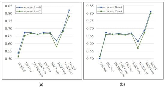
Figure 3. Comparison of the prediction performance between two similar courses (i.e., courses A and B) and two significantly different courses (i.e., courses A and C) in scenario 1 for all models. (a) Transfer from course A to courses B and C; (b) transfer from courses B and C to course A. The results show that all the models have better prediction performance for two similar courses than two significantly different courses.

To further verify this conclusion, we conducted an additional experiment on dataset II and dataset III (see Section 5.1 for details). The goal of this experiment is to quantitatively analyze the mechanism through which course similarity influences transfer effectiveness, rather than to compare classification performance directly. Therefore, we employ MAE, RMSE, and R-squared as evaluation metrics. These metrics are suited to measure the continuous error in the model’s predicted probabilities in the target course and to elucidate the relationship between this error and course similarity. As shown in Figure 4, course a and course b (and similarly, courses x and y) represent similar course pairs, whereas course a and course c (and courses x and z) represent dissimilar pairs. Notably, when the transfer training step is omitted, the transfer effect between the similar courses (a and b) remains marginally better than that between the dissimilar ones (a and c). This result substantiates that the content and nature of the courses have a significant impact on the model’s transfer effect.

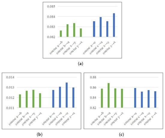
Figure 4. Comparison of cross-course prediction performance on the group of similar courses and the group of significantly different courses on datasets II and III. (a) MAE; (b) RMSE; and (c) R-squared. The results also show that models have better prediction performance between two similar courses than between two significantly different courses.

5.8. Cross-Course Performance Evolution Description (RQ4)

The evolution description of learning performance is an important application of the knowledge tracing model, which is a visual way to dynamically trace students’ performance. This task usually employs a heat-map to show the student’s level of performance. The cross-course performance evolution description also uses a heat-map to show the strength and weakness of each student’s mastery level of each KC on the source course and the target course.

Figure 5 shows the heat-map of the students in scenario 1 whose learning performance is constantly changing on certain KCs. Figure 5 comprises three sub-figures, which show the performance evolution of the same student in source course A and two target courses, i.e., course B and course C, respectively.

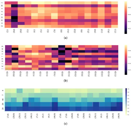
Figure 5. Visualization of a common student’s knowledge tracing. (a) MOOPer course A; (b) MOOPer course B; and (c) MOOPer course C.

For each sub-figure in Figure 5, the label in the vertical dimension denotes KCs. The horizontal dimension shows a sequence of KCs and corresponding answers (0 indicates incorrectly answered and 1 indicates correctly answered) from the source course, where the labels refer to the KCs input into the model at each time step. The heat-map color indicates the predicted probability that the student will demonstrate the corresponding KCs correctly in the next step. We observed the evolution of the predicted values for the five KCs in source course A. As Figure 5a shows, after answering the 20 exercises, the student improves these five KCs. Furthermore, Figure 5b shows that the prediction on KC 58 in target course B also improves as the learning progresses. However, as Figure 5c shows, the student masters KCs 28 and 20 but fails to master KCs 7 and 4, and there is no noticeable improvement on KC 46.

5.9. Visualization of Student Embedding (RQ5)

We employ T-SNE to visualize the representations of common students and distinct students in six courses after dimensionality reduction, as shown in Figure 6, where the area of the two color scatters in each figure reflects the number of students in each course.

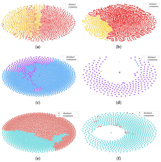
Figure 6. Visualization of common and distinct students’ embeddings in the different courses. (a) MOOPer course A; (b) MOOPer course B; (c) MOOC-Cube course a; (d) MOOC-Cube course b; (e) MOOC-Cube course x; and (f) MOOC-Cube course y.

For instance, Figure 6a,b show the difference between the MOOPer courses A and B. The relative positions of the representations of the common students and the distinct students are similar in the low-dimensional space; that is, the representations of the common students are mostly distributed on the left side of the figure, and the representations of the distinct students are mostly distributed on the right side of the figure. Figure 6c,e show that in course a and course x of MOOC-Cube, the representation distributions of the common and distinct students are relatively clustered. In addition, Figure 6d,f show that in course b and course y of MOOC-Cube, the number of common students is much higher than that of distinct students, but the representation of the distinct students is also relatively concentrated. However, Figure 6d,f also show that the representation distribution of the distinct students overlaps more with that of the common students. A reason may be that the distinct student representations of the target course (i.e., course b and course y) are more affected by the common students when training in the cross-domain stage.

6. Conclusions and Future Work

In this paper, we propose a cross-course knowledge tracing model. Through comparative experiments with different KT models, the superiority of MCKT in performance has been demonstrated. Of course, our method still has some limitations. After enhancing the model’s cross-course learning capability, its predictive performance can be somewhat affected by information from other courses, making it difficult to surpass single-target knowledge tracing. Our next objective is to trace these effects and develop methods to filter out “noise” introduced by other courses. Here, “noise” refers not to data errors, but to irrelevant information originating from source courses, which can hinder or mislead the prediction of knowledge states in the target course during cross-domain transfer—a phenomenon commonly termed “negative transfer”. Currently, our graph embedding layer utilizes the Doc2Vec model to obtain textual representations. However, our future work will prioritize architectural simplification and efficiency. Instead of pre-training methods, we will shift our focus towards exploring end-to-end trainable and lightweight alternatives. This includes investigating unified architectures, such as fine-tuning pre-trained language models or employing graph neural networks capable of jointly processing textual and structural information in a differentiable manner. Similarly, for graph representation learning, rather than simply substituting Node2Vec with other similar sampling-based methods, we plan to explore integrating trainable graph encoding layers that can be optimized jointly with the sequential model, thereby moving towards a more streamlined, efficient pipeline. The proposed MCKT model still carries potential risks in practical applications, primarily manifested in external threats from the following two aspects: First, the multi-stage pipeline—relying on separate Doc2Vec and Node2Vec modules—creates a dependency on pre-trained, fixed representations. The performance is sensitive to the parameters of these independent stages , and any noise or bias introduced during graph construction or text processing may propagate through the model. Second, the specific architecture of the fusion MLP and the LSTM is one of many possible configurations; while ablation studies validate our design, the causal link between the fusion mechanism itself and the performance gain could be further isolated from the specific hyperparameters selected. The main external threat comes from the applicability of the courses. Our evaluation was conducted on specific MOOC datasets. Although we selected courses from different disciplines such as IT, physics, history, and management, it is ultimately impossible to cover all disciplines. In addition, the computational complexity of the current process poses a significant threat to its feasibility in real-time educational environments, where low-latency predictions are usually required.

References

- Piech, C.; Bassen, J.; Huang, J.; Ganguli, S.; Sahami, M.; Guibas, L.J.; Sohl-Dickstein, J. Deep knowledge tracing. In Proceedings of the Advances in Neural Information Processing Systems, Montreal, QC, Canada, 7–12 December 2015; pp. 505–513. [Google Scholar]
- Shen, S.; Liu, Q.; Chen, E.; Wu, H.; Huang, Z.; Zhao, W.; Su, Y.; Ma, H.; Wang, S. Convolutional Knowledge Tracing: Modeling Individualization in Student Learning Process. In Proceedings of the the 43rd International ACM SIGIR Conference on Research and Development in Information Retrieval, Virtual, 25–30 July 2020; pp. 1857–1860. [Google Scholar]
- Pu, S.; Yudelson, M.; Ou, L.; Huang, Y. Deep Knowledge Tracing with Transformers. In Proceedings of the Artificial Intelligence in Education, Ifrane, Morocco, 6–10 July 2020; pp. 252–256. [Google Scholar]
- Yang, Y.; Shen, J.; Qu, Y.; Liu, Y.; Wang, K.; Zhu, Y.; Zhang, W.; Yu, Y. GIKT: A Graph-Based Interaction Model for Knowledge Tracing. In Proceedings of the Machine Learning and Knowledge Discovery in Databases—European Conference, ECML PKDD 2020, Ghent, Belgium, 14–18 September 2020; Volume 12457, pp. 299–315. [Google Scholar]
- Feng, W.; Tang, J.; Liu, T.X. Understanding Dropouts in MOOCs. In Proceedings of the The Thirty-Third AAAI Conference on Artificial Intelligence, Honolulu, HI, USA, 27 January–1 February 2019; pp. 517–524. [Google Scholar]
- Corbett, A.T.; Anderson, J.R. Knowledge tracing: Modeling the acquisition of procedural knowledge. User Model.-User-Adapt. Interact. 1994, 4, 253–278. [Google Scholar] [CrossRef]
- Lin, C.; Chi, M. Intervention-bkt: Incorporating instructional interventions into bayesian knowledge tracing. In Proceedings of the International Conference on Intelligent Tutoring Systems, Zagreb, Croatia, 7–10 June 2016; pp. 208–218. [Google Scholar]
- Wang, L.; Sy, A.; Liu, L.; Piech, C. Deep knowledge tracing on programming exercises. In Proceedings of the Fourth ACM Conference on Learning@ Scale, Cambridge, MA, USA, 20–21 April 2017; pp. 201–204. [Google Scholar]
- Mongkhonvanit, K.; Kanopka, K.; Lang, D. Deep Knowledge Tracing and Engagement with MOOCs. In Proceedings of the 9th International Conference on Learning Analytics and Knowledge, Tempe, AZ, USA, 4–8 March 2019; pp. 340–342. [Google Scholar]
- Zhang, J.; Shi, X.; King, I.; Yeung, D. Dynamic Key-Value Memory Networks for Knowledge Tracing. In Proceedings of the 26th International Conference on World Wide Web, Perth, Australia, 3–7 April 2017; pp. 765–774. [Google Scholar]
- Jiang, B.; Wei, Y.; Zhang, T.; Zhang, W. Improving the performance and explainability of knowledge tracing via Markov blanket. Inf. Process. Manag. 2024, 61, 103620. [Google Scholar] [CrossRef]
- Shukla, P.K.; Veerasamy, B.D.; Alduaiji, N.; Addula, S.R.; Sharma, S.; Shukla, P.K. Encoder only attention-guided transformer framework for accurate and explainable social media fake profile detection. Peer Peer Netw. Appl. 2025, 18, 232. [Google Scholar] [CrossRef]
- Wu, Z.; Liu, Y.; Cen, J.; Zheng, Z.; Xu, G. A cross-domain knowledge tracing model based on graph optimal transport. World Wide Web 2025, 28, 10. [Google Scholar] [CrossRef]
- Cheng, S.; Liu, Q.; Chen, E.; Zhang, K.; Huang, Z.; Yin, Y.; Huang, X.; Su, Y. AdaptKT: A Domain Adaptable Method for Knowledge Tracing. In Proceedings of the WSDM ’22: The Fifteenth ACM International Conference on Web Search and Data Mining, Virtual, 21–25 February 2022; pp. 123–131. [Google Scholar]
- Wilson, G.; Cook, D.J. A Survey of Unsupervised Deep Domain Adaptation. ACM Trans. Intell. Syst. Technol. 2020, 11, 51. [Google Scholar] [CrossRef] [PubMed]
- Huang, Y.; Huang, W.; Tong, S.; Huang, Z.; Liu, Q.; Chen, E.; Ma, J.; Wan, L.; Wang, S. STAN: Adversarial Network for Cross-domain Question Difficulty Prediction. In Proceedings of the IEEE International Conference on Data Mining, ICDM 2021, Auckland, New Zealand, 7–10 December 2021; pp. 220–229. [Google Scholar]
- Wu, Z.; Liang, Q.; Zhan, Z. Course Recommendation Based on Enhancement of Meta-Path Embedding in Heterogeneous Graph. Appl. Sci. 2023, 13, 2404. [Google Scholar] [CrossRef]
- Wu, Z.; Huang, L.; Huang, Q.; Huang, C.; Tang, Y. SGKT: Session graph-based knowledge tracing for student performance prediction. Expert Syst. Appl. 2022, 206, 117681. [Google Scholar] [CrossRef]
- Liu, A.; Wei, Y.; Xiu, Q.; Yao, H.; Liu, J. How Learning Time Allocation Make Sense on Secondary School Students’ Academic Performance: A Chinese Evidence Based on PISA 2018. Behav. Sci. 2023, 13, 237. [Google Scholar] [CrossRef] [PubMed]
- Ozyildirim, G. Time Spent on Homework and Academic Achievement: A Meta-analysis Study Related to Results of TIMSS. Psicol. Educ. 2022, 28, 13–21. [Google Scholar] [CrossRef]
- Le, Q.; Mikolov, T. Distributed Representations of Sentences and Documents. In Proceedings of the the 31st International Conference on International Conference on Machine Learning, ICML’14, Beijing, China, 21–26 June 2014; Volume 32, pp. 1188–1196. [Google Scholar]
- Grover, A.; Leskovec, J. node2vec: Scalable Feature Learning for Networks. In Proceedings of the 22nd ACM SIGKDD International Conference on Knowledge Discovery and Data Mining, San Francisco, CA, USA, 13–17 August 2016; pp. 855–864. [Google Scholar]
- Jansen, B.J.; Jung, S.; Salminen, J. Finetuning Analytics Information Systems for a Better Understanding of Users: Evidence of Personification Bias on Multiple Digital Channels. Inf. Syst. Front. 2024, 26, 775–798. [Google Scholar] [CrossRef]
- Bochkovskiy, A.; Wang, C.Y.; Liao, H.Y.M. YOLOv4: Optimal Speed and Accuracy of Object Detection. arXiv 2020, arXiv:2004.10934. [Google Scholar] [CrossRef]
- Dengsheng, C.; Li, J.; Xu, K. AReLU: Attention-based Rectified Linear Unit. arXiv 2020, arXiv:2006.13858. [Google Scholar]
- Liu, K.; Zhao, X.; Tang, J.; Zeng, W.; Liao, J.; Tian, F.; Zheng, Q.; Huang, J.; Dai, A. MOOPer: A Large-Scale Dataset of Practice-Oriented Online Learning. In Proceedings of the Knowledge Graph and Semantic Computing: Knowledge Graph Empowers New Infrastructure Construction—6th China Conference, CCKS 2021, Guangzhou, China, 4–7 November 2021; Volume 1466, pp. 281–287. [Google Scholar]
- Yu, J.; Luo, G.; Xiao, T.; Zhong, Q.; Wang, Y.; Feng, W.; Luo, J.; Wang, C.; Hou, L.; Li, J.; et al. MOOCCube: A Large-scale Data Repository for NLP Applications in MOOCs. In Proceedings of the The 58th Annual Meeting of the Association for Computational Linguistics, ACL 2020, Online, 5–10 July 2020; pp. 3135–3142. [Google Scholar]
- Manning, C.D.; Surdeanu, M.; Bauer, J.; Finkel, J.R.; Bethard, S.; McClosky, D. The Stanford CoreNLP Natural Language Processing Toolkit. In Proceedings of the the 52nd Annual Meeting of the Association for Computational Linguistics, ACL 2014, Baltimore, MD, USA, 22–27 June 2014; pp. 55–60. [Google Scholar]
- Chen, Y.; Liu, Q.; Huang, Z.; Wu, L.; Chen, E.; Wu, R.; Su, Y.; Hu, G. Tracking Knowledge Proficiency of Students with Educational Priors. In Proceedings of the the 2017 ACM on Conference on Information and Knowledge Management, Singapore, 6–10 November 2017; pp. 989–998. [Google Scholar]
- Li, P.; Tuzhilin, A. DDTCDR: Deep Dual Transfer Cross Domain Recommendation. In Proceedings of the WSDM ’20: The Thirteenth ACM International Conference on Web Search and Data Mining, Houston, TX, USA, 3–7 February 2020; pp. 331–339. [Google Scholar]
Disclaimer/Publisher’s Note: The statements, opinions and data contained in all publications are solely those of the individual author(s) and contributor(s) and not of MDPI and/or the editor(s). MDPI and/or the editor(s) disclaim responsibility for any injury to people or property resulting from any ideas, methods, instructions or products referred to in the content. |
© 2026 by the authors. Licensee MDPI, Basel, Switzerland. This article is an open access article distributed under the terms and conditions of the Creative Commons Attribution (CC BY) license.