A Multi-Time-Scale Coordinated Scheduling Model for Multi-Energy Complementary Power Generation System Integrated with High Proportion of New Energy Including Electricity-to-Hydrogen System

Abstract

It has become an urgent problem to deal with the uncertain influence caused by the high proportion of new energy connected to the grid and improve the consumption level of new energy in the background of the new power system. Based on the constantly updated predicted information of wind power, photovoltaic power, and load power, a multi-time-scale coordinated scheduling model for a multi-energy complementary power generation system integrated with a high proportion of new energy, including an electricity-to-hydrogen system, is proposed. The complex nonlinear factors in the operation cost of thermal power and pumped storage power generation were converted into a mixed integer linear model for solving the problem. The results show that the participation of the pumped storage units in the power grid dispatching can effectively alleviate the peak regulation and reserve pressure of the thermal power units. The electricity-to-hydrogen system has the advantages of fast power response and a wide adjustment range. Pumped storage plant, together with the electricity-to-hydrogen system, enhances the flexible adjustment ability of the power grid on the power side and the load side, respectively. The coordinated dispatch of the two can take into account the safety and economy of the power grid operation, maintain the power balance of the high-proportion new energy power generation system, and effectively reduce green power abandonment and improve the consumption level of clean energy.

1. Introduction

In response to global climate change and the growing demand for energy transition, accelerating the development of a clean, low-carbon, safe, and efficient modern energy system has gradually become a shared goal and guiding direction for global energy development [1,2].

To address the uncertainties [3] introduced by the integration of renewable energy and to ensure its efficient utilization, multi-energy complementary generation systems have emerged. Current research in this field primarily focuses on two aspects: output modeling of uncertain energy forecasts [4,5] and the analysis of complementary characteristics among energy sources [6,7]. By integrating and optimizing heterogeneous energy resources, multi-energy complementary generation systems can effectively offset the drawbacks of individual generation units, enhance resource utilization, and ensure the safe and reliable operation of the overall system [8].

With the rapid growth in renewable energy, the uncontrollability of new energy generation and the limited capacity of power transmission have led to severe curtailment of green electricity. The complementary operation of conventional power sources can only mitigate the fluctuations of wind and solar outputs, but cannot fully resolve the issue of renewable energy absorption. The advancement in energy storage technologies provides a new approach to addressing large-scale wind and solar curtailment. Among these, pumped storage power stations play an indispensable role in enhancing renewable energy utilization, thanks to their fast start–stop capability, flexible operation, and strong peak-shaving performance [9]. A growing body of research has explored the joint optimal scheduling of pumped storage with other power sources. For instance, Reference [10] proposed a coordinated scheduling strategy for pumped storage and wind power, effectively reducing wind curtailment. Reference [11] developed a method combining pumped storage and battery energy storage to smooth photovoltaic output fluctuations, thereby facilitating large-scale solar integration and improving the system’s low-carbon economic performance. Reference [12] introduced a day-ahead optimization strategy for thermal units, storage, and loads, where controlling the state of pumped storage capacity enhances its peak-shaving effectiveness.

The aforementioned studies primarily focus on the generation-side regulation capabilities of multi-energy complementary systems without accounting for the flexible regulation potential on the demand side under the framework of the new power system. Power-to-hydrogen (P2H) systems enhance system flexibility by using hydrogen storage tanks to buffer through hydrogen storage and release, thereby smoothing load fluctuations. As a type of flexible load, P2H systems can participate in demand response, promoting the mutual complementarity between electricity and hydrogen and enabling broader energy optimization. In the optimization of renewable-based power systems, the current research mainly emphasizes the role of P2H processes in renewable energy absorption and in maintaining power supply–demand balance [13,14].

However, the above studies mainly consider scheduling at a single time-scale and do not adequately capture the uncertainty characteristics of wind and solar power forecasts across different time-scales. With the large-scale integration of intermittent energy sources such as wind and solar into the power grid, coordinated optimization across multiple time-scales is essential to progressively mitigate forecast deviations and enhance renewable energy absorption capability. In this regard, Reference [15] proposed a multi-time-scale coordinated scheduling strategy for wind, solar, hydro, and thermal power, which continuously updates forecast data and dynamically revises day-ahead plans to maintain accurate load tracking and maximize complementarity. Reference [16] focused on day-ahead and intra-day rolling optimization between wind farms and pumped storage systems, leveraging updated forecasts and storage flexibility to improve joint operation benefits. Reference [17] developed a multi-time-scale optimization model for source–storage–grid coordinated scheduling in an electricity–hydrogen hybrid storage system and verified its feasibility. Reference [18] incorporated hydrogen demand into a multi-time-scale low-carbon optimization strategy that accounts for electricity–gas–heat–hydrogen demand response. At present, most multi-time-scale scheduling studies involving power-to-hydrogen systems remain confined to integrated energy systems, with limited research addressing their role in high-renewable power systems.

To address the above issues, this study proposes a multi-time-scale coordinated scheduling model for a high-renewable multi-energy complementary generation system incorporating power-to-hydrogen (P2H). The model integrates continuously updated forecasts of wind power, photovoltaic output, and load demand to construct a three-stage coordinated scheduling framework, encompassing day-ahead (24 h), intra-day (1 h), and real-time (15 min) horizons. The complex nonlinear operational costs of thermal and pumped storage units are linearized into a mixed-integer linear programming (MILP) formulation. Case studies based on a modified IEEE 10-unit system are conducted to examine the flexible regulation capabilities of pumped storage and P2H systems, thereby verifying the effectiveness of the proposed multi-time-scale coordinated scheduling approach.

The main contributions of this paper are summarized as follows.

(1)

A unified multi-time-scale coordinated scheduling framework is proposed for a high-renewable multi-energy complementary power generation system that simultaneously integrates pumped storage units and a power-to-hydrogen (P2H) system. Different from existing studies that mainly focus on single time-scale scheduling or integrated energy systems, the proposed framework explicitly coordinates day-ahead (24 h), intra-day (1 h), and real-time (15 min) scheduling stages, fully exploiting the progressive improvement of wind power, photovoltaic power, and load forecasting accuracy across time-scales.

(2)

The complementary roles of pumped storage and P2H are jointly modeled within the same power system scheduling framework. Pumped storage units are treated as fast-response bidirectional regulation resources on the generation side, while the P2H system is modeled as a flexible demand-side resource that can rapidly adjust its power consumption through hydrogen production and storage. Their coordinated participation in multi-time-scale scheduling is quantitatively analyzed in terms of renewable energy curtailment, spinning reserve requirements, and thermal unit operating costs.

(3)

To ensure computational tractability, the nonlinear operating characteristics of thermal power units and pumped storage units, including start-up/shutdown costs and operating costs, are reformulated into a mixed-integer linear programming (MILP) model through a unified linearization approach. This allows the proposed multi-time-scale scheduling problem to be efficiently solved using commercial solvers, making the framework suitable for practical power system applications.

(4)

Comprehensive case studies based on a modified IEEE 10-unit system are conducted to validate the effectiveness of the proposed approach. Multiple operational scenarios and different wind–solar penetration levels are investigated, demonstrating the advantages of the proposed multi-time-scale coordinated scheduling framework in enhancing renewable energy accommodation, reducing system operating costs, and improving overall system flexibility.

2. Basic Framework of Multi-Time-Scale Coordinated Scheduling

The forecasting accuracy of wind power, photovoltaic generation, and load improves gradually as the time-scale decreases. By utilizing continuously updated forecasting information, a multi-time-scale coordinated scheduling model for a high-proportion renewable energy power system with power-to-hydrogen is established, aiming to minimize the total operating cost while considering both system economy and efficient utilization of clean energy. As a secondary energy form complementary to electricity, hydrogen energy is expected to play a key role in future low-carbon energy systems. In this paper, the power-to-hydrogen system is regarded only as a flexible load participating in power demand response, which, together with pumped storage and thermal power units, provides flexible regulation resources for the high-proportion wind and solar integrated system. The role and value of renewable hydrogen production as a flexible load in power system scheduling are further explored.

The basic framework of multi-time-scale scheduling is described as follows:

(1)

Day-ahead scheduling model: Executed once every 24 h with a resolution of 1 h. Based on one-day-ahead forecast data of wind power, photovoltaic generation, and load, the generation plans of wind, solar, thermal, pumped storage, and power-to-hydrogen units for the next 24 h are optimized. The start-up and shutdown plans of thermal power units are treated as known parameters and are input into the intra-day and real-time scheduling models.

(2)

Intra-day 1 h scheduling model: Executed once every hour with a resolution of 15 min, totaling 24 executions per day. Based on one-hour-ahead forecast data of wind power, photovoltaic generation, and load, and using the start-up and shutdown plans of thermal units determined in the day-ahead scheduling, this model takes the day-ahead thermal generation plan as a reference and optimizes the generation plans of wind, solar, and power-to-hydrogen units for the next hour, as well as the start-up, shutdown, and generation plans of pumped storage units and the intra-day correction plan for thermal unit output. The intra-day start-up, shutdown, and generation plans of pumped storage units and the output correction plan of thermal units are treated as known parameters and are input into the real-time scheduling model.

(3)

Real-time 15 min scheduling model: Executed once every 15 min with a resolution of 15 min, totaling 96 executions per day. Based on 15 min ahead forecast data of wind power, photovoltaic generation, and load, as well as the start-up and shutdown plans of thermal units determined in the day-ahead scheduling and those of pumped storage units determined in the intra-day scheduling, this model takes the intra-day output correction plans of thermal and pumped storage units as references and optimizes the generation plans of wind, solar, and power-to-hydrogen units for the next 15 min, as well as the real-time output correction plans of thermal and pumped storage units.

The coordination relationship among day-ahead, intra-day, and real-time scheduling is shown in Figure 1. In Figure 1, the black and gray blocks under different time-scale scheduling plans represent the resolution of the current scheduling period.

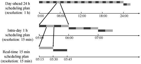
Figure 1. The relationship between day-ahead dispatch, in-day dispatch, and real-time dispatch.

3. Multi-Time-Scale Coordinated Scheduling Model

3.1. Day-Ahead Scheduling Model

3.1.1. Objective Function

The day-ahead scheduling model aims to minimize the total operating cost of the system. The total operating cost of the system includes the power generation cost of thermal power units (sum of the coal consumption cost and the start-up and shutdown cost of thermal power units), the start-up and shutdown loss cost of pumped storage units, and the penalty cost for wind and solar power curtailment, which is specifically expressed as

$$f_1=\min \left(C_H+C_q+C_{ps}+C_A\right)$$

(1)

$$\left\{\begin{array}{l}{C}_H={\displaystyle \sum _{t=1}^{\mathrm{NT}}{\displaystyle \sum _{g=1}^{\mathrm{NG}}{U}_{g,t}\left(a_g{P}_{g,t}^2+b_g{P}_{g,t}+c_g\right)}}\\ C_q={\displaystyle \sum _{t=1}^{\mathrm{NT}}{\displaystyle \sum _{g=1}^{\mathrm{NG}}{S}_q\left(U_{g,t-1}\left(1-U_{g,t}\right)+U_{g,t}\left(1-U_{g,t-1}\right)\right)}}\\ C_{ps}={\displaystyle \sum _{t=1}^{\mathrm{NT}}{\displaystyle \sum _{j=1}^{\mathrm{NJ}}\left\{\begin{array}{l}{S}_{on}\cdot \left[I_{j,t}^g(1-I_{j,t-1}^g)+I_{j,t}^p(1-I_{j,t-1}^p)\right]\\ +S_{off}\cdot \left[I_{j,t-1}^g(1-I_{j,t}^g)+I_{j,t-1}^p(1-I_{j,t}^p)\right]\end{array}\right\}}}\\ C_A={\displaystyle \sum _{t=1}^{\mathrm{NT}}\left({\lambda }_w{A}_{w,t}+{\lambda }_v{A}_{v,t}\right)}\end{array}\right.$$

(2)

where $f_1$ is the total operating cost of the day-ahead scheduling model; $C_H$ is the coal consumption cost of thermal power units; $C_q$ is the start-up and shutdown costs of thermal power units; $C_{ps}$ is the operating cost of the pumped storage unit; $C_A$ is the punishment cost of wind and solar power curtailment. $\mathrm{NT}$ is the total number of time periods within the scheduling cycle. $\mathrm{NG}$ is the total number of thermal power units. $\mathrm{NJ}$ is the total number of pumped storage units. $a_g$, $b_g$, $c_g$ are the coal consumption cost coefficients of thermal power unit g, respectively. $P_{g,t}$ is the active power of the thermal power unit g in the t period of the day-ahead dispatching model. $U_{g,t}$ is a binary variable representing the operating status of the thermal power unit g in period t, $U_{g,t}=0$ indicating shutdown and $U_{g,t}=1$ indicating operation. $S_q$ is the start-up and shutdown costs of the thermal power unit g. $S_{on}$ and $S_{off}$ are the start-up–shutdown cost coefficient of the pumped storage unit, respectively; $I_{j,t}^g$ and $I_{j,t}^p$ are the 0–1 state variable of whether the pumped storage unit j is in the power generation mode or the pumping mode during the t period, 1 is taken as yes and 0 as no. ${\lambda }_w$ is the cost coefficient of wind power curtailment penalty; $A_{w,t}$ is the abandoned wind power during t period; ${\lambda }_v$ is the cost coefficient of solar abandonment penalty; $A_{v,t}$ is the abandoned solar power during t period.

3.1.2. Constraints

(1)

Constraints on wind and solar power output

To explicitly characterize the uncertainty of renewable generation, the forecasted wind and photovoltaic power outputs at different time-scales are represented using confidence intervals. Specifically, the available power range is defined as

$$\left\{\begin{array}{l}{P}_{\max }=\mu +k\sigma \\ P_{\min }=\mu -k\sigma \end{array}\right.$$

(3)

where μ and σ denote the predicted mean value and standard deviation, respectively, and k is the confidence coefficient. In this study, k is set to 1.96, corresponding to a 95% confidence level. As the scheduling time-scale shortens from day-ahead to intra-day and real-time stages, the forecasting accuracy improves, and the associated uncertainty intervals become progressively narrower, reflecting the updated prediction information.

In the multi-energy complementary system optimization scheduling model, the uncertainty of wind power output is usually described in the form of confidence intervals. Therefore, the wind power output modeling is as follows:

$$0\le P_{w,t}\le P_{w,N}$$

(4)

$$P_{w,\min ,t}\le P_{w,t}\le P_{w,\max ,t}$$

(5)

$$\left\{\begin{array}{l}{P}_{w,t}^{up}={\mu }_{w,t}+1.96{\sigma }_{w,t}\\ P_{w,t}^{dn}={\mu }_{w,t}-1.96{\sigma }_{w,t}\end{array}\right.$$

(6)

$$\left\{\begin{array}{l}{P}_{w,\max ,t}=\min \left\{P_{w,t}^{up},P_{w,N}\right\}\\ P_{w,\min ,t}=\max \left\{0,P_{w,t}^{dn}\right\}\end{array}\right.$$

(7)

$$A_{w,t}=P_{w,\max ,t}-P_{w,t}$$

(8)

where $P_{w,N}$ is the installed capacity of the wind farm; $P_{w,t}$ is the output of wind power dispatching in the t period; $P_{w,\max ,t}$ and $P_{w,\min ,t}$ are the upper and lower limits of the available power of the wind farm in the t period, which are determined based on the confidence intervals of the corresponding forecasts. $P_{w,t}^{up}$, $P_{w,t}^{dn}$ is the prediction of the upper and lower limits of the wind farm in the t period. ${\mu }_{w,t}$, ${\sigma }_{w,t}$ are the mean and standard deviation of the predicted output probability distribution of the wind farm in period t, respectively. If the output power range of wind power is too large, it will reduce the economic efficiency of system optimization and dispatching, and even make the dispatching model unsolvable. Therefore, the output range of wind power and photovoltaic power generation is set $\left[{\mu }_{w,t}-1.96{\sigma }_{w,t},{\mu }_{w,t}+1.96{\sigma }_{w,t}\right]$ to ensure that at least 95% of the wind and solar output can be utilized. The output modeling of photovoltaic power generation is consistent with that of wind power, as mentioned above, and will not be elaborated further.

(2)

Operational constraints of thermal power units

a. Output constraints of thermal power units

$$U_{g,t}{P}_{g,\min }\le P_{g,t}\le U_{g,t}{P}_{g,\max }$$

(9)

where $P_{g,\max }$, $P_{g,\min }$ are the upper and lower limits of the output of the thermal power unit g, respectively.

b. Output climbing constraint of thermal power units

$$\left\{\begin{array}{l}{P}_{g,t}-P_{g,t-1}\le R_g^U{U}_{g,t-1}\\ P_{g,t-1}-P_{g,t}\le R_g^D{U}_{g,t}\end{array}\right.$$

(10)

where $R_g^U$ is the climbing rate of the thermal power unit g (hourly level); $R_g^D$ is the downhill climbing rate (hourly level) of the thermal power unit g.

c. Minimum start-up and shutdown time constraints for thermal power units

$$\left\{\begin{array}{l}\left(U_{g,t-1}-U_{g,t}\right)\left(T_{g,t-1}^{\mathrm{on}}-T_{g,\min }^{\mathrm{on}}\right)\ge 0\\ \left(U_{g,t}-U_{g,t-1}\right)\left(T_{g,t-1}^{\mathrm{off}}-T_{g,\min }^{\mathrm{off}}\right)\ge 0\end{array}\right.$$

(11)

where $T_{g,t-1}^{\mathrm{on}}$, $T_{g,t-1}^{\mathrm{off}}$ are the periods when the thermal power unit has been continuously started up and shut down from g to t − 1, respectively. $T_{g,\min }^{\mathrm{on}}$, $T_{g,\min }^{\mathrm{off}}$ are the minimum continuous start-up and shutdown times of the thermal power unit g, respectively.

d. Constraints of reserve capacity of thermal power units [19]

$$\left\{\begin{array}{l}{P}_{g,t}+R_{g,t}^{up}\le P_{g,\max }{U}_{g,t}\\ P_{g,t}-R_{g,t}^{dn}\ge P_{g,\min }{U}_{g,t}\end{array}\right.$$

(12)

where $R_{g,t}^{up}$, $R_{g,t}^{dn}$ are the reserved upward and downward reserve capacities of the thermal power unit g in period t to cope with the uncertainty of wind and solar output, respectively.

(3)

Operational constraints of pumped storage power stations

a. Output constraints of pumped storage units

$$\left\{\begin{array}{l}{I}_{j,t}^g{P}_{j,\min }^g\le P_{j,t}^g\le I_{j,t}^g{P}_{j,\max }^g\\ I_{j,t}^p{P}_{j,\min }^p\le P_{j,t}^p\le I_{j,t}^p{P}_{j,\max }^p\end{array}\right.$$

(13)

where $P_{j,t}^g$, $P_{j,t}^p$ are the power generation and pumping power of the pumped storage unit j in time period t, respectively; $P_{j,\max }^g$, $P_{j,\min }^g$ are the maximum and minimum power generation capacities of the pumped storage unit j, respectively. $P_{j,\max }^p$, $P_{j,\min }^p$ are the maximum and minimum pumping powers of the pumped storage unit j, respectively.

b. Operating condition constraints of the pumped storage unit

$$I_{j,t}^g+I_{j,t}^p\le 1$$

(14)

$$\left\{\begin{array}{l}{\displaystyle \sum _{j=1,j\ne j^{\prime }}^{\mathrm{NJ}}{I}_{j,t}^g}\le \left(\mathrm{NJ}-1\right)-\left(\mathrm{NJ}-1\right)I_{j^{\prime },t}^p\\ {\displaystyle \sum _{j=1,j\ne j^{\prime }}^{\mathrm{NJ}}{I}_{j,t}^p}\le \left(\mathrm{NJ}-1\right)-\left(\mathrm{NJ}-1\right)I_{j^{\prime },t}^g\end{array}\right.$$

(15)

Equation (14) ensures that a single pumped storage unit cannot operate simultaneously in both power generation and water pumping modes. In addition, there is a pressure water pipe between the upper reservoir and the pump-turbine of a pumped storage power station. Therefore, regardless of the number of pumped storage units, it cannot operate in both power generation and water pumping modes simultaneously. In other words, if at least one pumped storage unit is operating in the power generation mode, then no other unit can operate in the pumping mode at the same time, and vice versa. Equation (15) represents the mutually exclusive operating conditions of the pumped storage unit group at the same time.

c. Water volume constraints of pumped storage power stations

$$X_t=X_{t-1}+{\displaystyle \sum _{j=1}^{\mathrm{NJ}}\left({\eta }_j^{pum}{P}_{j,t}^p-{\eta }_j^{gen}{P}_{j,t}^g\right)}$$

(16)

$$X_{\min }\le X_t\le X_{\max }$$

(17)

$$X_T=X_0$$

(18)

where $X_t$ is the storage capacity of the upper reservoir of the pumped storage power station during period t; ${\eta }_j^{gen}$, ${\eta }_j^{pum}$ are the average water volume/electricity conversion coefficients of the pumped storage unit j during power generation and water pumping, respectively. $X_{\max }$, $X_{\min }$ are the maximum and minimum water storage capacities of the upper reservoir of the pumped storage power station, respectively. $X_0$ is the initial storage capacity of the upper reservoir; $X_T$ is the storage capacity of the upper reservoir at the end of the term. Equation (18) ensures the daily operational energy balance of the upper reservoir of the pumped storage power station.

d. Reserve capacity constraints of pumped storage units [19].

$$\left\{\begin{array}{l}{P}_{j,t}^g+R_{j,t}^{gu}\le P_{j,\max }^g{I}_{j,t}^g\\ P_{j,t}^g-R_{j,t}^{gd}\ge P_{j,\min }^g{I}_{j,t}^g\end{array}\right.$$

(19)

$$\left\{\begin{array}{l}{P}_{j,t}^p+R_{j,t}^{pu}\le P_{j,\max }^p{I}_{j,t}^p\\ P_{j,t}^p-R_{j,t}^{pd}\ge P_{j,\min }^p{I}_{j,t}^p\end{array}\right.$$

(20)

where $R_{j,t}^{gu}$, $R_{j,t}^{gd}$ are the upper and lower reserve capacities provided by the pumped storage unit j in the t period under the power generation condition, respectively. $R_{j,t}^{pu}$, $R_{j,t}^{pd}$ are the upper and lower reserve capacities provided by the pumped storage unit j in the t period under the pumping condition, respectively.

(4)

Constraints of the electric hydrogen production system

a. Power constraint of electrolyzer

$$P_{\min }^{P2H}{u}_t^{P2H}\le P_t^{P2H}\le P_{\max }^{P2H}{u}_t^{P2H}$$

(21)

where $P_t^{P2H}$ is the hydrogen production power at time t; $P_{\max }^{P2H}$, $P_{\min }^{P2H}$ are the upper and lower limits of hydrogen production power; and $u_t^{P2H}$ is the hydrogen production condition status indicator of the electric hydrogen production system at time t, 1 indicates that it is in the corresponding state, and 0 indicates that it is not in the corresponding state. It can represent two operating states: hydrogen production and idle.

b. Constraints of hydrogen storage capacity

$$M_t=M_{t-1}+{\eta }_{P2H}{P}_t^{P2H}{\gamma }_{eh}-O_t$$

(22)

$$O_t\ge 0$$

(23)

$$M_{\min }\le M_t\le M_{\max }$$

(24)

$$M_0=M_{end}$$

(25)

where ${\eta }_{P2H}$ is the energy conversion efficiency of hydrogen production by electricity; ${\gamma }_{eh}$ is the coefficient representing the conversion from hydrogen energy to hydrogen capacity; $M_t$ is the hydrogen storage capacity in the hydrogen storage tank at time t; $M_{\min }$, $M_{\max }$ are the minimum and maximum hydrogen capacity that the electric hydrogen production system can store, respectively; and $M_0$, $M_{end}$ are hydrogen reserves for the initial and final periods, respectively. $O_t$ is the hydrogen directly delivered from the hydrogen storage tank at time t. Equation (25) ensures that the hydrogen storage can be cycled periodically within the dispatching period to guarantee the long-term sustainable operation of the system.

c. Intra-day hydrogen load demand constraint

$${\displaystyle \sum }_{t=1}^{NT}{O}_t^{\prime }=H_{Load}$$

(26)

where $H_{Load}$ is the hydrogen load demand. Equation (26) requires that the total amount of hydrogen delivered externally within the system cycle should meet the hydrogen load demand.

(5)

System constraints

a. Power balance constraint

$$P_{\mathrm{w},t}^{\mathrm{day}}+P_{\mathrm{v},t}^{\mathrm{day}}+{\displaystyle \sum _{g=1}^{\mathrm{NG}}{P}_{g,t}^{\mathrm{day}}+}{\displaystyle \sum _{j=1}^{\mathrm{NJ}}\left(P_{j,t}^{\mathrm{g},\mathrm{day}}-P_{j,t}^{\mathrm{p},\mathrm{day}}\right)}-P_{\mathrm{P}2\mathrm{H},t}^{\mathrm{day}}=P_{\mathrm{L},t}^{\mathrm{day}}$$

(27)

where $P_{\mathrm{w},t}^{\mathrm{day}}$ is the dispatching output of the wind farm in the t period as planned in the day-ahead plan. $P_{\mathrm{v},t}^{\mathrm{day}}$ is the dispatching output of the photovoltaic power station in the t period as planned in the day-ahead plan; $P_{g,t}^{\mathrm{day}}$ is the dispatching output of thermal power unit g in the t period in the day-ahead plan; $P_{j,t}^{\mathrm{g},\mathrm{d}\mathrm{a}\mathrm{y}}$ and $P_{j,t}^{\mathrm{p},\mathrm{d}\mathrm{a}\mathrm{y}}$ are the power generation and pumping power of the pumped storage unit j under the day-ahead dispatching plan, respectively; $P_{\mathrm{P}2\mathrm{H},t}^{\mathrm{day}}$ is the hydrogen production power of the planned electric hydrogen production system in the day-ahead plan; and $P_{\mathrm{L},t}^{\mathrm{day}}$ is the load predicted one day in advance for the t period.

b. Spinning reserve demand constraint

$$\left\{\begin{array}{l}{\displaystyle \sum _{g=1}^{\mathrm{NG}}{R}_{g,t}^{\mathrm{up}}}+{\displaystyle \sum _{j=1}^{\mathrm{NJ}}\left(R_{j,t}^{\mathrm{gu}}+R_{j,t}^{\mathrm{pd}}\right)}\ge \alpha \left(P_{\mathrm{w},t}-P_{\mathrm{w},\min ,t}\right)+\beta \left(P_{\mathrm{v},t}-P_{\mathrm{v},\min ,t}\right)\\ {\displaystyle \sum _{g=1}^{\mathrm{NG}}{R}_{g,t}^{\mathrm{dn}}}+{\displaystyle \sum _{j=1}^{\mathrm{NJ}}\left(R_{j,t}^{\mathrm{gd}}+R_{j,t}^{\mathrm{pu}}\right)}\ge \alpha \left(P_{\mathrm{w},\max ,t}-P_{\mathrm{w},t}\right)+\beta \left(P_{\mathrm{v},\max ,t}-P_{\mathrm{v},t}\right)\end{array}\right.$$

(28)

where $\alpha$, $\beta$ are the reserve demand coefficients considering the uncertainty of the current wind power and photovoltaic output, respectively, approximately 15–25% [20].

c. Capacity constraints of transmission lines

$$-L_{l,\max }\le {\displaystyle \sum _{m=1}^M{G}_{l,m}{P}_{m,t}\le L_{l,\max }}$$

(29)

where m is the node number; M is the total number of nodes; $G_{l,m}$ the transfer distribution factor from node m to line l; $P_{m,t}$ is the power injected into the active power of node m in time period t; and $L_{l,\max }$ is the maximum transmission power of line l.

3.2. Intra-Day Scheduling Model

3.2.1. Objective Function

Since the day-ahead dispatching model has already optimized the start-up and shutdown plans for thermal power units in the next 24 h, the intra-day dispatching model need not take into account the start and stop situations of thermal power units. By adjusting the deviation in the wind, solar and load forecast from the power generation unit’s output consumption date to the day. Intra-day dispatching model aims to minimize the total operating cost of the system within the dispatching cycle, including the coal consumption cost of thermal power units, the output adjustment cost of thermal power units, the start–stop loss cost of pumped storage units, and the penalty cost for wind and solar power curtailment. Specifically, it is expressed as

$$f_2=\min \left(C_H+C_{\Delta pg}+C_{ps}+C_A\right)$$

(30)

$$\left\{\begin{array}{l}{C}_H={\displaystyle \sum _{t=t_0}^{t_0+N_T-1}{\displaystyle \sum _{g=1}^G{U}_{g,t}\left(a_g{P}_{g,t}^2+b_g{P}_{g,t}+c_g\right)}}\\ C_{\Delta pg}={\displaystyle \sum _{t=t_0}^{t_0+N_T-1}{\displaystyle \sum _{g=1}^G{S}_{pg}\Delta P_{g,t}^{hour}}}\\ C_{ps}={\displaystyle \sum _{t=t_0}^{t_0+N_T-1}{\displaystyle \sum _{j=1}^J\left\{\begin{array}{l}{S}_{on}\cdot \left[I_{j,t}^g(1-I_{j,t-1}^g)+I_{j,t}^p(1-I_{j,t-1}^p)\right]\\ +S_{off}\cdot \left[I_{j,t-1}^g(1-I_{j,t}^g)+I_{j,t-1}^p(1-I_{j,t}^p)\right]\end{array}\right\}}}\\ C_A={\displaystyle \sum _{t=t_0}^{t_0+N_T-1}\left({\lambda }_w{A}_{w,t}+{\lambda }_v{A}_{v,t}\right)}\end{array}\right.$$

(31)

where $f_2$ is the total operating cost of the intra-day scheduling model; $t_0$ is the initial period of the scheduling cycle; and $N_T$ is the total number of periods within the intra-day scheduling cycle (an intra-day one-hour scheduling cycle includes four 15 min periods). $S_{pg}$ is the cost of adjusting the output of thermal power units within one dispatching cycle; $\Delta P_{g,t}^{hour}$ is the adjustment of the cost coefficient for the unit output of thermal power units. The output adjustment amount of the thermal power unit g in the t period compared to the previous day can be expressed as $\Delta P_{g,t}^{hour}=\left|P_{g,t}^{hour}-P_{g,t}^{day}\right|$, where $P_{g,t}^{hour}$ is the power generation capacity of the thermal power unit g in the t period under the intra-day hourly dispatching plan.

3.2.2. Constraints

(1)

Constraints on wind and solar power output

With the advancement in the time-scale, the intra-day prediction level of wind and solar output has further improved. Therefore, the mean and standard deviation of the predicted output probability distribution in this constraint have been updated, but the form remains the same as before.

(2)

Operational constraints of thermal power units

Due to the adoption of the day-ahead start–stop plan for thermal power units, intra-day dispatching does not take into account the minimum start–stop time constraints of thermal power units. The output climbing constraint of the unit needs to be adjusted accordingly due to the change in the time-scale. The output constraints and reserve capacity constraints of thermal power units remain the same as before.

The output climbing constraint of thermal power units [21] is

$$\left\{\begin{array}{l}{P}_{g,t}^{hour}-P_{g,t-1}^{hour}\le {\displaystyle \frac{R_g^U}{4}}{U}_{g,t-1}\\ P_{g,t-1}^{hour}-P_{g,t}^{hour}\le {\displaystyle \frac{R_g^D}{4}}{U}_{g,t}\end{array}\right.$$

(32)

where $P_{g,t}^{hour}$ is the dispatching output of the thermal power unit g in the t period in the intra-day.

(3)

Operational constraints of pumped storage power stations

Pumped storage power stations that have undergone intra-day hourly rolling dispatching still follow the daily operating water balance constraint of the reservoir:

$$X_{24}^{hour}=X_0$$

(33)

where $X_{24}^{hour}$ is the water storage volume of the upper reservoir after hourly rolling dispatching in the 24th cycle at the end of the day.

The constraints for the remaining pumped storage power stations remain the same as before.

(4)

Constraints of the electric hydrogen production system

The constraint of the electric hydrogen production system is similar to the recent model and will not be elaborated here.

(5)

System constraints

The wind and solar reserve demand coefficients in the intra-day spinning reserve demand constraints have all been updated, but the form remains the same as before. The capacity constraint of the transmission line remains the same as before.

$$P_{w,t}^{hour}+P_{v,t}^{hour}+P_{g,t}^{hour}+{\displaystyle \sum _{j=1}^{NJ}\left(P_{j,t}^{g,hour}-P_{j,t}^{p,hour}\right)}-P_{P2H,t}^{hour}=P_{L,t}^{hour}$$

(34)

where $P_{w,t}^{hour}$ is the dispatching output of the wind farm in the t period in the intra-day model; $P_{v,t}^{hour}$ is the dispatching output of the photovoltaic power station in the t period in the intra-day model; $P_{j,t}^{g,hour}$ and $P_{j,t}^{p,hour}$ are the power generation and pumping power of the pumped storage unit j in the t period under the intra-day hourly dispatching plan, respectively; $P_{P2H,t}^{hour}$ is the hydrogen production power of the electric hydrogen production system in the t period of the in intra-day model; and $P_{L,t}^{hour}$ is the load predicted one hour in advance for the t period.

3.3. Real-Time Scheduling Model

3.3.1. Objective Function

In real-time dispatching, the start–stop status and output plan of thermal power units remain unchanged. The start–stop plan of pumped storage units is substituted into the real-time dispatching model, and the rapid regulation capacity of pumped storage units and the electric hydrogen production system are utilized to absorb the deviation in wind and solar load predictions at different time-scales within the day in real time. The real-time scheduling model aims to minimize the real-time operating cost of the system, including the real-time adjustment cost of the output of pumped storage units, the real-time adjustment cost of the output of the electro-hydrogen production system, and the penalty cost for wind and solar power curtailment. Specifically, it is expressed as

$$f_3=\min \left(C_{\Delta ps}+C_A\right)$$

(35)

$$\left\{\begin{array}{l}{C}_{\Delta ps}={\displaystyle \sum _{j=1}^J{S}_{ps}\Delta P_{j,t}^{realt}}\\ C_A={\lambda }_w{A}_{w,t}+{\lambda }_v{A}_{v,t}\end{array}\right.$$

(36)

where $f_3$ is the real-time operating cost of the system; $C_{\Delta ps}$ is the cost of adjustment in real time for the output of the pumped storage unit; $S_{ps}$ is the cost coefficient for the unit output adjustment of the pumped storage unit; and $\Delta P_{j,t}^{realt}$ is the real-time output adjustment amount of the pumped storage unit j in the t period compared to the intra-day dispatching plan, which can be further divided into the power generation and pumping power adjustment amounts under the same start–stop state of the pumped storage unit, that is $\Delta P_{j,t}^{realt}=\left|P_{j,t}^{g,realt}-P_{j,t}^{g,hour}\right|+\left|P_{j,t}^{p,realt}-P_{j,t}^{p,hour}\right|$, where $P_{j,t}^{g,realt}$ and $P_{j,t}^{p,realt}$ are the power generation and pumping power of the pumped storage unit j in the t period under the real-time dispatching plan, respectively.

3.3.2. Constraints

(1)

Constraints of wind and solar power output

With the advancement in the time-scale, the real-time prediction level of wind and solar output has further improved. Therefore, the mean and standard deviation of the predicted output probability distribution have been updated, but the form remains the same as before.

(2)

Operational constraints of thermal power units

Real-time dispatching remains the start–stop plan and output plan of thermal power units unchanged, and the output of thermal power units is carried out according to the intra-day dispatching results. Therefore, only the reserve capacity constraint of thermal power units is considered, as in the day-ahead Equation (12).

(3)

Operational constraints of pumped storage power stations

After real-time rolling dispatching, pumped storage power stations still follow the daily operating water balance constraint of the reservoir:

$$X_{96}^{realt}=X_0$$

(37)

where $X_{96}^{hour}$ is the storage volume of the upper reservoir after real-time rolling dispatching in the 96th cycle at the end of the day.

Since the start–stop status of the pumped storage units in the real-time dispatching model remains consistent with the intra-day plan, the operational condition constraints of the pumped storage units are not considered. The remaining constraints of the pumped storage power stations remain the same as day-ahead constraints.

(4)

Constraints of the electric hydrogen production system

The constraint of the electric hydrogen production system is similar to the day-ahead model, so it is not necessary to repeat.

(5)

System operation constraints

The wind and solar reserve demand coefficients in the real-time spinning reserve demand constraints have all been updated, but the form remains the same as the day-ahead model. The capacity constraint of the transmission line remains the same as day-ahead.

The output of the thermal power unit in the real-time dispatching plan is a known quantity and remains consistent with the result of the intra-day dispatching, which is $P_{g,t}^{hour}$. Therefore, the system power balance constraint in the real-time scheduling stage is

$$P_{w,t}^{realt}+P_{v,t}^{realt}+P_{g,t}^{hour}+{\displaystyle \sum _{j=1}^{NJ}\left(P_{j,t}^{g,realt}-P_{j,t}^{p,realt}\right)}-P_{P2H,t}^{realt}=P_{L,t}^{realt}$$

(38)

where $P_{w,t}^{realt}$ is the dispatching output of the wind farm in the real-time model during period t; $P_{v,t}^{realt}$ is the dispatching output of the photovoltaic power station in the real-time model during the t period; $P_{P2H,t}^{realt}$ is the hydrogen production power of the electric hydrogen production system in period t of the real-time model; and $P_{L,t}^{realt}$ is the load predicted 15 min in advance for the t period.

4. Case Analysis

4.1. Case Parameters

According to Reference [22], the integrated wind farm and photovoltaic (PV) station have a total installed capacity of 3300 MW with a capacity ratio of 2:1. The data for the ten thermal units are based on the standard IEEE 10-unit test system and are appropriately modified for this study [23].

The pumped storage power station consists of six variable-speed, constant-frequency units, each rated at 300 MW, resulting in a total installed capacity of 1800 MW. The unit parameters are configured with reference to the Bath County Pumped Storage Station in the United States [24]. The pumping and generating power of each unit is continuously adjustable, and detailed parameters are listed in Table 1.

Table 1. Parameters of pumped storage station.

$P_{j,\min }^{\mathrm{g}}$/MW	15	${\eta }_j^{\mathrm{p}}$/[m3(MWh)−1]	780
$P_{j,\max }^{\mathrm{g}}$/MW	300	$X_0$/107 m3	2
$P_{j,\min }^{\mathrm{p}}$/MW	30	$X_{\min }$/107 m3	1.06
$P_{j,\max }^{\mathrm{p}}$/MW	300	$X_{\max }$/107 m3	4.38
${\eta }_j^{\mathrm{g}}$/[m3(MWh)−1]	999	NJ	6

The electrolyzer has a rated power of 450 MW, with a minimum operating power set to 10% of its rated capacity. The power-to-hydrogen conversion efficiency ${\eta }_{\mathrm{P}2\mathrm{H}}$ is 76%, and the hydrogen-to-energy conversion coefficient ${\gamma }_{eh}$ is 260 Nm³/MW. The hydrogen storage tank has an upper capacity limit of 1.6 × 10⁶ Nm³ and a lower limit of 2 × 10⁵ Nm³, with an initial storage level of 8 × 10⁵ Nm³. The intra-day hydrogen load is set to 7.6 × 10⁵ Nm³.

The penalty cost for wind and PV curtailment is 300 USD/MWh, and the unit output adjustment cost coefficient is 100 USD/MW. The reserve requirements for wind and PV in the day-ahead, intra-day, and real-time scheduling stages are set to 20%, 5%, and 1%, respectively.

Figure 2 presents the forecast intervals of wind and PV output across different time-scales. Figure 3 illustrates the multi-time-scale load forecasting profiles.

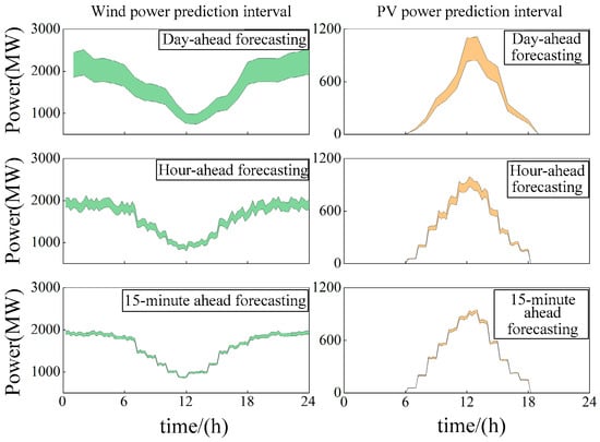
Figure 2. Predicted output range of wind power and photovoltaic in multi-time-scales.

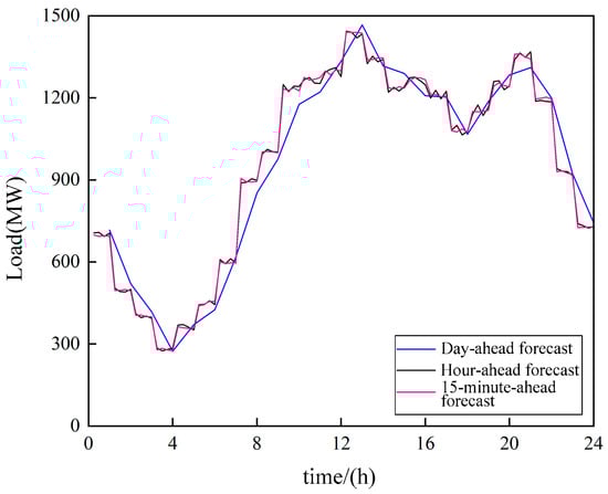
Figure 3. Predicted output of load in multi-time-scales.

4.2. Solution Method

The unit commitment problem is mathematically a non-convex and nonlinear mixed-integer programming problem that involves a large number of discrete and continuous variables. The coal consumption cost and minimum up/down time constraints of thermal units are linearized following the method described in Reference [25], and thus are not repeated here. The start-up cost of thermal units and the operating cost of pumped storage units share similar mathematical structures, and the same linearization principle applies.

To illustrate the linearization procedure, the start-up cost of a thermal unit is taken as an example. Let $U_{g,t}\cdot U_{g,t-1}$ denote the nonlinear term formed by the product of two binary variables. This nonlinearity can be removed by introducing an auxiliary binary variable and additional constraints [24]. By introducing a new binary variable $U_{G,t}$ and defining $U_{G,t}=U_{g,t}\cdot U_{g,t-1}$, the nonlinear expression can be equivalently converted into the following linear constraints:

$$\left\{\begin{array}{l}0\le U_{G,t}\le U_{g,t}\hfill \\ U_{G,t}\le U_{g,t-1}\hfill \\ U_{G,t}\ge U_{g,t}+U_{g,t-1}-1\hfill \end{array}\right.$$

(39)

The proposed multi-time-scale coordinated scheduling model is formulated as a mixed-integer linear programming (MILP) problem and solved using the commercial solver CPLEX 12.6. All simulations are conducted on a personal computer equipped with an Intel 2.6 GHz processor and 8 GB of RAM.

In the case studies, the day-ahead scheduling problem, which includes unit commitment decisions for thermal units, typically requires several tens of seconds to a few minutes to reach optimality, depending on the number of scenarios and renewable penetration levels. The intra-day scheduling problems, with a reduced decision space and fixed unit commitment status, are solved within several seconds per rolling horizon. The real-time scheduling problems, which mainly involve output adjustment decisions, can be solved in less than one second per 15 min interval.

These computational results demonstrate that the proposed framework is computationally tractable and suitable for practical applications. Moreover, the hierarchical multi-time-scale structure effectively distributes the computational burden across different stages, enabling timely implementation in real-world power system operations.

4.3. Analysis of Scheduling Results

To investigate the impact of different operational strategies on system optimization, the following four scenarios are considered:

Scenario 1: Pumped storage and power-to-hydrogen (P2H) are not included, and a multi-time-scale coordinated scheduling model for wind–solar–thermal generation is applied.

Scenario 2: Pumped storage is included while P2H is not, using a multi-time-scale coordinated scheduling model for wind–solar–thermal–pumped storage generation.

Scenario 3: Both pumped storage and P2H are included, adopting the proposed multi-time-scale coordinated scheduling model for wind–solar–thermal–pumped storage–P2H systems.

Scenario 4: Both pumped storage and P2H are included, but only a single-stage day-ahead scheduling model for the wind–solar–thermal–pumped storage–P2H system is used.

Table 2 presents the optimal scheduling results for the four scenarios over a one-day period.

Table 2. Optimal scheduling results of four methods within one day.

Scenarios	Thermal Power Generation Cost/USD	Wind Curtailment Penalty Cost/USD	Solar Curtailment Penalty Cost/USD	Thermal Power Upward Spinning Reserve Capacity/MW	Thermal Power Downward Spinning Reserve Capacity/MW
scenario 1	1,284,200	350,730	0	12,165	40,398
scenario 2	635,770	6890	0	7460	22,459
scenario 3	876,680	0	0	3447	8113
scenario 4	42,130	0	0	1030	2660

4.3.1. Impact Analysis of Pumped Storage on System Scheduling

To examine the impact of the pumped storage power station on system optimization, Scenarios 1 and 2 are compared. Figure 4 and Figure 5 show the on/off status of generating units across 96 time periods for the two scenarios, where thermal units are labeled G1–G10 and pumped storage units are labeled J1–J6. For clarity, blank regions in the figures indicate that a thermal unit or pumped storage unit is offline, whereas colored solid dots represent periods during which the units are in operation.

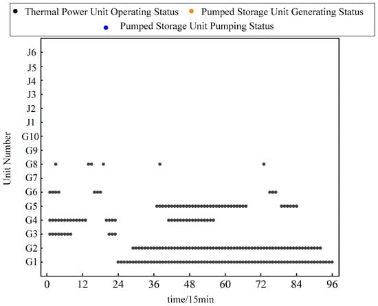
Figure 4. Unit commitment of method 1.

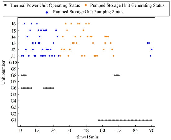
Figure 5. Unit commitment of method 2.

By comparing Figure 4 and Figure 5, together with Table 2 and the load profile in Figure 3, it can be observed that in Scenario 1—where no pumped storage units and no P2H system are included—thermal units G1, G2, G4, and G5 remain online for extended periods during the peak-load interval from periods 28 to 68 (i.e., 07:00 to 17:00). These units primarily supply the base-load demand, and during this period, the system relies entirely on thermal units to provide reserve capacity to cope with the uncertainty of wind and solar generation.

In Scenario 2, however, the pumped storage units are able to share part of the reserve requirement. As shown in Figure 5, the inclusion of pumped storage during peak-load hours significantly reduces the number of thermal units that must be online. This alleviates the peak-shaving burden on thermal units, prevents large fluctuations in their scheduled output, and effectively reduces the frequency of unit start-ups and shutdowns induced by wind and PV variability.

In addition, the participation of pumped storage units reduces the generation cost of thermal units by approximately 27%, contributing to safer and more economical system operation.

Solar PV plants generate during the daytime and shut down at night, enabling them to track load variations effectively and exhibit positive peak-shaving characteristics. As a result, PV output is fully utilized in both scenarios, and the PV curtailment penalty cost in Table 2 is zero. In contrast, wind power exhibits a typical anti-peak-shaving pattern, leading to significant wind curtailment in Scenario 1 and substantially increasing the total system operating cost.

Meanwhile, in Scenario 2, the pumped storage units provide flexible bidirectional regulation, consuming electricity to pump water during low-load periods and converting curtailed wind energy into stored gravitational potential energy for later generation during peak-load hours. Consequently, the wind curtailment penalty cost in Scenario 2 is much lower than that in Scenario 1, indicating that the participation of pumped storage in system scheduling significantly enhances renewable energy utilization and reduces curtailment.

In summary, the integration of pumped storage effectively improves the operational performance of thermal units, yields notable economic benefits, and enhances the utilization and accommodation of clean energy.

4.3.2. Analysis of the Impact of Power-to-Hydrogen on System Scheduling

To investigate the impact of power-to-hydrogen (P2H) as a flexible hydrogen load on system optimization, Scenarios 2 and 3 are compared. Figure 6 illustrates the scheduling results of the pumped storage units and thermal units in Scenario 2, while Figure 7 presents the full-resource scheduling results for Scenario 3. Both figures are generated using the 96 data points obtained from the multi-time-scale scheduling results.

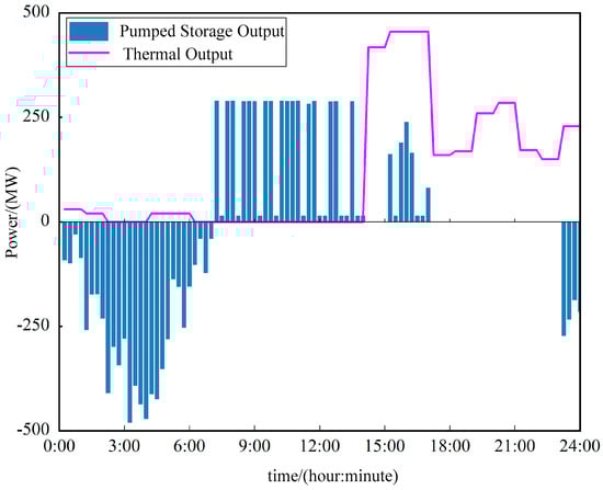
Figure 6. Partial scheduling results of method 2.

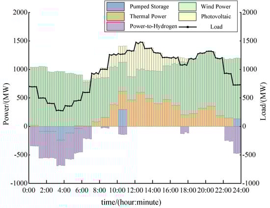
Figure 7. Scheduling results of method 3.

The key difference between Scenarios 3 and 2 lies in the participation of the P2H system in the multi-time-scale optimization process in Scenario 3. A comparison of the two figures shows that the integration of P2H leads to a noticeable reduction in the number of operating pumped storage units and an increase in the number of online thermal units. This occurs because, while satisfying the intra-day hydrogen demand, the P2H system behaves as a flexible load that increases the overall system demand. Consequently, additional thermal units must be committed, and the number of pumped storage units operating in pumping mode is reduced to accommodate the higher load. As shown in Table 2, this results in higher thermal generation costs and a reduction in the upward/downward spinning reserve capacity provided by thermal units in Scenario 3 compared with Scenario 2.

It should be clarified that in Scenario 3, the P2H system introduces an additional flexible hydrogen load on top of the original electricity demand. Therefore, the total system demand in Scenario 3 consists of both the base electrical load and the hydrogen production demand, whereas Scenario 2 only considers the electrical load.

As a result, the observed increase in thermal power generation cost in Scenario 3 does not indicate a deterioration of the scheduling strategy. Instead, it reflects the increased total energy demand required to support hydrogen production. Importantly, this additional demand is supplied while completely eliminating wind curtailment and enhancing renewable energy utilization. From a system-wide perspective, Scenario 3 achieves a trade-off between higher energy conversion demand and improved clean energy accommodation and multi-energy coupling benefits.

Furthermore, the inclusion of P2H reduces wind curtailment costs to zero in Scenario 3, indicating that P2H can rapidly track fluctuations in wind and solar output and adjust its power consumption accordingly. This capability not only enhances renewable energy utilization but also improves the overall operational flexibility of the system.

4.3.3. Analysis of the Impact of Time-Scales on System Scheduling

To examine the impact of different time-scales on system scheduling, Scenarios 3 and 4 are compared. Figure 8 illustrates the full-resource scheduling results for Scenario 4. Since Scenario 4 adopts only day-ahead scheduling, the horizontal axis contains 24 data points.

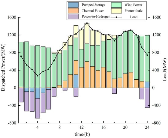
Figure 8. Scheduling results of method 4.

By comparing Figure 7 and Figure 8, it is evident that as the scheduling framework shifts from single day-ahead scheduling to the proposed day-ahead–intra-day–real-time multi-time-scale approach, the power adjustments of both the pumped storage units and the P2H system become more rapid. This increased responsiveness enables the system to compensate for deviations between the 15 min ahead forecasts of wind, solar, and load and the predictions from the previous time-scale. These results demonstrate that the proposed multi-time-scale scheduling method effectively leverages the fast response speed and wide regulation range of both pumped storage and P2H systems, thereby enhancing the system’s flexible regulation capability on both the generation and load sides.

4.3.4. Impact Analysis of Wind–Solar Penetration on System Scheduling

Table 3 presents the optimal scheduling results over 96 time periods for the proposed multi-time-scale coordinated scheduling model with P2H under different wind–solar penetration levels. The case studies under different renewable penetration levels can also be interpreted as validations using multiple datasets, which helps demonstrate the robustness and generality of the proposed scheduling framework. The total installed capacities of thermal units (1662 MW) and pumped storage (1800 MW) are kept constant, while increases in the combined installed capacity of the wind farm and PV plant lead to higher wind–solar penetration.

Table 3. Optimal scheduling results of method 3 under different wind and solar penetration rates.

Total Installed Capacity of Wind and Solar PV/MW	Wind and Solar PV Penetration Rate	Total System Operating Cost (×104)/USD	Thermal Power Generation Cost (×104)/USD	Pumped Storage Operating Cost (×104)/USD	Renewable Curtailment Penalty Cost (×104)/USD	Total Up and Down Spinning Reserve Capacity from Thermal Power /MW
3960	53.4%	56.44	35.22	20.97	2.54	116,883
3300	48.8%	84.73	63.58	21.08	0.69	91,639
2750	44.3%	144.9	123.11	21.79	0	65,903
2200	38.8%	208.19	186.64	21.55	0	39,903
1650	32.3%	279.59	258.9	20.69	0	22,029
1100	24.1%	387.64	367.55	20.09	0	15,487

Neglecting the operating cost of P2H, the overall system operating cost gradually decreases as more zero-marginal-cost wind and solar generation is integrated, thereby alleviating the output requirements of thermal units and reducing their generation cost. As wind–solar penetration increases, the pumped storage station and the P2H system jointly provide flexible power regulation to mitigate fluctuations in renewable output and load, enabling the system to better absorb renewable energy. Wind–solar curtailment penalties occur only when the penetration level reaches 48.8%.

Moreover, higher wind–solar penetration amplifies the uncertainty associated with renewable output, requiring thermal units to provide additional spinning reserve to ensure the safe and stable operation of the high-renewable multi-energy complementary system. These results indicate that the proposed multi-time-scale scheduling framework performs consistently well across multiple data sets represented by different renewable penetration levels, demonstrating its robustness and general applicability.

5. Conclusions

To address the challenge of large-scale renewable energy integration in the context of new power systems, this study proposes a multi-time-scale coordinated scheduling model for high-renewable power systems incorporating power-to-hydrogen (P2H) technology. Considering that the forecasting accuracy of wind power, photovoltaic generation, and load demand improves as the time horizon shortens, a three-stage coordination framework—day-ahead, intra-day, and real-time—is established. The main conclusions are as follows:

(1)

The P2H system can rapidly follow fluctuations in wind and solar generation to meet overall system load requirements, thereby enhancing system flexibility from the demand side.

(2)

The joint participation of pumped storage and P2H systems in multi-time-scale coordinated scheduling effectively balances grid security and economic performance. This cooperation substantially reduces renewable energy curtailment and improves the overall utilization of clean energy.

To ensure computational tractability and focus on multi-time-scale coordinated scheduling, several simplifying assumptions are adopted. The fuel prices of thermal units are assumed to be fixed over the scheduling horizon, and fuel price uncertainties are not considered. In addition, generation unit availability is assumed to be deterministic, and unexpected outages are neglected.

Network constraints are modeled using a DC power flow formulation based on power transfer distribution factors (PTDFs), which ignores reactive power, voltage constraints, and transmission losses. Moreover, the power-to-hydrogen (P2H) system and pumped storage units are assumed to be perfectly controllable within their technical limits, without considering operational delays, degradation, or control uncertainties.

These assumptions do not affect the qualitative insights of this study but indicate potential directions for future work, such as incorporating market uncertainties, equipment reliability, and resilience-oriented scheduling under extreme operating conditions.

While this study focuses on centralized multi-time-scale economic dispatch under normal operating conditions, several promising research directions can be pursued in future work to further enhance the applicability and robustness of the proposed framework.

First, the proposed scheduling model can be extended toward a multi-agent cooperative operation framework that explicitly considers the heterogeneous profit motives and contribution differences in independent stakeholders, such as wind farms and P2H systems. By introducing incentive-compatible profit allocation mechanisms, for example, through asymmetric Nash bargaining, the coordination between different participants can be enhanced to support long-term cooperation in integrated energy systems.

Second, to improve system robustness against renewable generation uncertainty and extreme operating conditions, distributionally robust optimization techniques can be incorporated into the multi-time-scale scheduling framework. Uncertainty sets constructed using data-driven or fuzzy-set-based methods, such as the imprecise Dirichlet model, would allow flexible control of conservatism while maintaining low-carbon and economic operation.

Third, the current framework can be further expanded toward resilience-oriented scheduling and restoration under extreme scenarios or grid faults. In this context, cross-sector flexible resources, including demand-side flexibility (e.g., building thermal inertia) and mobile energy storage (e.g., electric buses in transportation networks), can be jointly coordinated with power system resources to enhance system resilience.

Finally, to address the increasing scale and coupling complexity of future integrated energy and transportation systems, decentralized or asynchronous solution algorithms, such as ADMM-based approaches, can be investigated to improve computational efficiency and scalability. These extensions would enable the proposed framework to better support resilient, market-oriented, and large-scale practical applications.

References

- Pastore, L.M.; de Santoli, L. Socio-economic implications of implementing a carbon-neutral energy system: A Green New Deal for Italy. Energy 2025, 322, 135682. [Google Scholar] [CrossRef]
- Mararakanye, N.; Bekker, B. Renewable energy integration impacts within the context of generator type, penetration level and grid characteristics. Renew. Sustain. Energy Rev. 2019, 108, 441–451. [Google Scholar] [CrossRef]
- Xu, M.; Li, W.B.; Feng, Z.J.; Wang, J.X.; Yu, G.Z.; Li, W.T.; Li, Z.Y. Economic dispatch model of high proportional new energy grid-connected consumption considering source load uncertainty. Energies 2023, 16, 1696. [Google Scholar] [CrossRef]
- Wang, Y.S.; Liu, Y.Z.; Kirschen, D.S. Scenario reduction with submodular optimization. IEEE Trans. Power Syst. 2017, 32, 2479–2480. [Google Scholar] [CrossRef]
- Bertsimas, D.; Litvinov, E.; Sun, X.A.; Zhao, J.Y.; Zheng, T.X. Adaptive robust optimization for the security constrained unit com-mitment problem. IEEE Trans. Power Syst. 2013, 28, 52–63. [Google Scholar] [CrossRef]
- Lu, L.; Yuan, W.; Xu, H.Y.; Li, Y.B.; Lin, K.R.; Wang, H.Y.; Zhang, M.M.; Zhang, J. Evaluation of the complementary characteristics for Wind-Photovoltaic-Hydro hybrid system considering multiple uncertainties in the medium and long term. Water Resour. Manag. 2024, 38, 793–814. [Google Scholar] [CrossRef]
- Yan, J.; Qu, T.; Han, S.; Liu, Y.; Lei, X.; Wang, H. Reviews on characteristic of renewables: Evaluating the variability and complementarity. Int. Trans. Electr. Energy Syst. 2020, 30, e12281. [Google Scholar] [CrossRef]
- Hrinchenko, H.; Kupriyanov, O.; Khomenko, V.; Khomenko, S.; Kniazieva, V. An approach to ensure operational safety for renewable energy equipment. In Circular Economy for Renewable Energy; Springer Nature: Cham, Switzerland, 2023; pp. 1–17. [Google Scholar]
- Xiang, C.; Xu, X.; Zhang, S. Current situation of small and medium-sized pumped storage power stations in Zhejiang Province. J. Energy Storage 2024, 78, 110070. [Google Scholar] [CrossRef]
- Yuan, W.; Xin, W.; Su, C.; Cheng, C.; Yan, D.; Wu, Z. Cross-regional integrated transmission of wind power and pumped-storage hydropower considering the peak shaving demands of multiple power grids. Renew. Energy 2022, 190, 1112–1126. [Google Scholar] [CrossRef]
- Naval, N.; Yusta, J.M.; Sánchez, R. Optimal scheduling and management of pumped hydro storage integrated with grid-connected renewable power plants. J. Energy Storage 2023, 73, 108993. [Google Scholar] [CrossRef]
- Wu, Z.; Wang, J.Z.; Peng, S.; Liu, Y.F.; Liu, D.; Li, X.; Ma, Z.Q.; Zhang, L.P. Flexibility Assessment of Ternary Pumped Storage in Day-Ahead Optimization Scheduling of Power Systems. Appl. Sci. 2024, 14, 8820. [Google Scholar] [CrossRef]
- Shash, A.Y.; Abdeltawab, N.M.; Hassan, D.M.; Hassan, M.A.; Salem, M.M.; Mohamed, A.M.; Mohamed, H.A.; EI-Sebaie, M.M. Computational methods, artificial intelligence, modeling, and simulation applications in green hydrogen production through water electrolysis: A review. Hydrogen 2025, 6, 21. [Google Scholar] [CrossRef]
- Huang, H.; Sun, G.; Chen, S.; Wei, Z.; Zang, H. Peer-to-peer energy trading of hydrogen-producing prosumers in power distribution network. Sustain. Energy Technol. Assess. 2025, 75, 104221. [Google Scholar] [CrossRef]
- Zhang, D.; Du, T.; Yin, H.; Xia, S.; Zhang, H. Multi-time-scale coordinated operation of a combined system with wind-solar-thermal-hydro power and battery units. Appl. Sci. 2019, 9, 3574. [Google Scholar] [CrossRef]
- He, J.; Sun, B.; Jia, Q.; Xu, F.; Gao, B. Research on intraday rolling optimal dispatch including pumped storage power station. In Proceedings of the 2020 International Conference on Intelligent Computing, Automation and Systems (ICICAS), Chongqing, China, 11–13 December 2020; pp. 261–265. [Google Scholar]
- Li, D.S.; Qian, K.; Xu, Y.Y.; Zhou, J.S.; Wang, Z.F.; Peng, Y.F.; Xing, Q. A Multi-Time Scale Optimal Scheduling Strategy for the Electro-Hydrogen Coupling System Based on the Modified TCN-PPO. Energies 2025, 18, 1926. [Google Scholar] [CrossRef]
- Tang, J.; Liu, J.F.; Sun, T.X.; Kang, H.R.; Hao, X.Q. Multi-time-scale optimal scheduling of integrated energy system considering demand response. IEEE Access 2023, 11, 135891–135904. [Google Scholar] [CrossRef]
- Kim, W.J.; Lee, Y.S.; Chun, Y.H.; Ro, K.S. Reserve-constrained unit commitment considering adjustable-speed pumped-storage hydropower and its economic effect in Korean power system. Energies 2022, 15, 2386. [Google Scholar] [CrossRef]
- Zhou, B.; Geng, G.; Jiang, Q. Hydro-thermal-wind coordination in day-ahead unit commitment. IEEE Trans. Power Syst. 2016, 31, 4626–4637. [Google Scholar] [CrossRef]
- Chen, P.; Tian, Z.; Zhang, Y.; Wang, H.; Wang, W.; Liu, J. Research on new energy consumption methods using optimized dispatch of thermal power units. In Journal of Physics: Conference Series, 2024 3rd International Conference on Smart Energy and Electrical Engineering (SEEE 2024), Harbin, China, 20–22 December 2024; IOP Publishing: Bristol, UK, 2025; Volume 3000, p. 12057. [Google Scholar] [CrossRef]
- Kulyk, M.; Zgurovets, O. Modeling of power systems with wind, solar power plants and energy storage. In Systems, Decision and Control in Energy I; Springer International Publishing: Cham, Switzerland, 2020; pp. 231–245. [Google Scholar]
- Ding, H.J.; Hu, Z.C.; Song, Y.H. Stochastic optimization of the daily operation of wind farm and pumped-hydro-storage plant. Renew. Energy 2012, 48, 571–578. [Google Scholar] [CrossRef]
- Rosenlieb, E.; Heimiller, D.; Cohen, S. Closed-Loop Pumped Storage Hydropower Resource Assessment for the United States; Final Report on HydroWIRES Project D1: Improving Hydropower and PSH Representations in Capacity Expansion Models; National Renewable Energy Lab (NREL): Golden, CO, USA, 2022. [Google Scholar]
- Guisández, I.; Pérez-Díaz, J.I. Mixed integer linear programming formulations for the hydro production function in a unit-based short-term scheduling problem. Int. J. Electr. Power Energy Syst. 2021, 128, 106747. [Google Scholar] [CrossRef]
Disclaimer/Publisher’s Note: The statements, opinions and data contained in all publications are solely those of the individual author(s) and contributor(s) and not of MDPI and/or the editor(s). MDPI and/or the editor(s) disclaim responsibility for any injury to people or property resulting from any ideas, methods, instructions or products referred to in the content. |
© 2026 by the authors. Licensee MDPI, Basel, Switzerland. This article is an open access article distributed under the terms and conditions of the Creative Commons Attribution (CC BY) license.