AI and Evolutionary Computation for Intelligent Aviation Health Monitoring

Abstract

This paper presents a novel framework integrating evolutionary computation and artificial intelligence for aircraft health monitoring and management systems. The research addresses critical challenges in modern aircraft maintenance through a comprehensive approach combining real-time fault detection, predictive maintenance, and multi-objective optimization. The framework employs deep learning models for fault detection, achieving about 97% classification accuracy with an F1-score of 0.97, while remaining useful life prediction yields an R² score of 0.89 with a mean absolute error of 9.8 h. Evolutionary algorithms optimize maintenance strategies, reducing downtime and costs by up to 22% compared to traditional methods. The methodology includes robust data processing protocols, feature engineering techniques, and a modular system architecture supporting real-time monitoring and decision-making. Simulation experiments demonstrate the framework’s effectiveness in balancing maintenance objectives while maintaining high reliability. The research provides practical implementation guidelines and addresses key challenges in computational efficiency, data quality, and system integration. The results show significant improvements in maintenance planning efficiency and system reliability compared to traditional approaches. The framework’s modular design enables scalability and adaptation to various aircraft systems, offering broader applications in complex technical system maintenance.

1. Introduction

1.1. Background and Motivation

In aerospace and other high-stakes industries, the reliability of technical systems is paramount. Modern aircraft, for instance, are equipped with engines, avionics, hydraulic networks, and other interlinked subsystems that collectively handle immense workloads under demanding conditions. Each subsystem is monitored by numerous sensors, generating vast amounts of data in real time. This influx of continuously updated information presents both an opportunity and a challenge. On one hand, it provides a granular view of an aircraft’s operational status, potentially allowing early detection of performance deviations. On the other hand, the sheer volume and complexity of sensor data can overwhelm traditional rule-based systems and manual inspection approaches.

Classical health monitoring strategies, often built on static rules or periodic checks, can miss subtle patterns that develop gradually or occur in non-linear ways [1]. As systems become more interconnected, isolated signals may no longer convey the complete picture of an impending issue. Manual inspections, while necessary for certain procedures, cannot feasibly analyze real-time data streams for every subsystem. Consequently, failures can remain undetected until they escalate, leading to costly downtime or, worse, safety incidents. These limitations underscore the urgency for more advanced, data-driven solutions capable of handling complex interactions and adapting to evolving operating conditions.

Complex technical systems, such as those found in modern aircraft, face a multitude of potential failure modes across their various subsystems. Detecting these faults early, diagnosing their root causes, and accurately predicting when they may escalate pose significant challenges. This difficulty arises from the complexity of system interdependencies, the sheer volume and variety of sensor data, and the dynamic nature of operating environments (e.g., differing flight conditions, wear rates, or maintenance practices). Traditional, rule-based methods often struggle to capture nuanced interactions among components or adapt quickly to emerging faults—particularly when they exhibit subtle, non-linear behaviors.

In contrast, artificial intelligence (AI) and evolutionary computation (EC) offer robust, data-driven approaches that inherently handle complexity and adapt to new information over time [2]. AI models can learn from historical and real-time data to identify patterns indicative of incipient failures, while EC algorithms optimize these models (and associated decision-making processes) in the face of numerous, potentially conflicting objectives. Collectively, AI and EC can deliver more accurate predictions, earlier fault detection, and automated strategies for maintenance decisions, significantly improving both reliability and cost-effectiveness in high-stakes domains like aerospace.

This study aims to develop and evaluate an AI-driven framework, augmented by evolutionary computation, for health monitoring, fault detection, and predictive maintenance of complex technical systems. Specifically, the work focuses on four objectives: (1) investigating how evolutionary algorithms (such as genetic algorithms) can identify sensor features most relevant for fault detection; (2) exploring a range of AI techniques for anomaly detection and fault classification; (3) demonstrating how AI-based models can estimate remaining useful life (RUL) to inform maintenance schedules; and (4) employing multi-objective evolutionary algorithms to balance safety, cost, and operational constraints. The research addresses several key questions: how evolutionary algorithms can be used to optimize feature sets, model hyperparameters, and maintenance decisions; which AI architectures yield the most accurate and robust fault detection; and how predictive maintenance policies, driven by AI models, can effectively reduce downtime and minimize costs in real-world settings.

1.2. Related Works

The field of evolutionary computation began with groundbreaking research introducing genetic algorithms [3]. This discipline [4] includes various problem-solving approaches inspired by biological evolution and genetics. Genetic algorithms represent the most recognized evolutionary computation method [5,6], developing multiple potential solutions simultaneously. Each solution appears as a string of bits—known as the genotype—with its effectiveness measured by a fitness function that evaluates the bit-string’s performance for the specific problem (converting genotype to phenotype). The evolution process uses operators like mutation, crossover, and selection to guide solution development across generations.

The field has expanded to include numerous computational methods, such as genetic programming [7], evolution strategies [8], differential evolution [9,10], evolutionary programming [11], permutation-based evolutionary algorithms [12], memetic algorithms [13], distribution estimation algorithms [14], particle swarm optimization [15], interactive evolutionary algorithms [16], ant colony optimization [17,18], and artificial immune systems [19], plus other variations [20,21]. One key advantage of evolutionary algorithms is their natural adaptation to parallel processing [22,23,24], making them ideal for modern multi-processor computing systems. The field rests on substantial theoretical foundations covering convergence analysis [25,26,27], parameter optimization and management [28], and sophisticated fitness landscape evaluation tools [29,30,31], including fitness-distance relationships [32] and landscape mathematical analysis [33], among others. These theoretical principles guide the practical implementation of evolutionary solutions. Additionally, numerous open-source software packages support evolutionary computation across different programming languages [34,35,36,37,38,39,40,41,42,43], simplifying the application of these algorithms to new challenges and fields.

Evolutionary computation has proven successful in addressing various types of problems across multiple domains, including multi-objective optimization [44,45,46,47], data science [48], machine learning [49,50,51], classification [52], feature selection [53], neural architecture search [54], neuroevolution [55], bioinformatics [56], scheduling [57], algorithm selection [58], computer vision [59], hardware validation [60], software engineering [61,62], and multi-task optimization [63,64], plus many other applications.

In the aviation sector, aircraft maintenance has emerged as a crucial focus area, largely because of its significant influence on operational expenses. The MRO operations constitute a fundamental part of airlines’ cost structure, representing approximately 10% of their total operational expenses [65]. The fundamental challenge of aircraft maintenance involves servicing each aircraft at designated maintenance facilities after completing specific numbers of flights, where necessary maintenance, repairs, and overhaul work is conducted according to manufacturer specifications, aviation authority requirements, and specific airline protocols [66]. This process becomes more complex due to various operational factors including flight schedule disruptions, fleet availability, aircraft usage patterns, and maintenance facility capacity constraints. The situation is further complicated by the nature of aviation parts manufacturing, which involves sophisticated, limited-run production delivering precisely engineered components typically manufactured to specific order requirements [67].

The paper [68] provides a comprehensive examination of prior research of AI in aviation domain. A groundbreaking IoT and machine learning method for anticipating aircraft wing anti-icing system thermal behavior is introduced in [69]. Testing revealed this neural network-based approach to be more effective and faster than conventional fluid dynamics calculations, indicating its potential value in aviation applications.

Research [70] examines statistical and machine learning applications for more effective, precise, and data-centered analysis of aircraft environmental effects including fuel consumption, emissions, and noise levels. It outlines primary research areas, key studies, and possibilities for further incorporating these methods to enhance aviation sustainability.

Research [71] suggests implementing deep neural networks and transfer learning to examine aircraft lap joint images for automated corrosion detection with accuracy like human inspectors, potentially supporting maintenance staff and enabling more automated condition-based maintenance systems.

The research [72] examines helicopter vibration control, specifically focusing on individual blade control (IBC) for reducing hub vibration. By combining various approaches including fuzzy neural networks, the study indicates that IBC effectively reduces hub vibrations, providing key insights for helicopter vibration control system design.

Four data-driven systems for predicting aeroengine exhaust gas temperature baselines, crucial for engine health monitoring and flight safety, are presented in [73]. Real engine data were used to train machine learning models, with the generalized regression neural network demonstrating superior accuracy and efficiency, making it ideal for airline operations.

Study [74] analyzes machine learning applications in lithium-ion battery research, particularly in materials development, health monitoring, and problem diagnosis, emphasizing aviation batteries and environmentally friendly aviation technology. The research evaluates various machine learning approaches’ strengths and limitations to advance understanding and development in this area.

Research [75] demonstrates machine learning applications, particularly multilayer perceptron networks, for modeling aero engine transient performance, emphasizing heat transfer during transitional operations. This model, developed using finite element simulation data and enhanced with actual engine measurements, effectively simulates engine thermal transitions.

A data-driven method for predicting suddenly expanded flow base pressure, which influences aerodynamic vehicle base drag, is outlined in [76]. Using machine learning models trained on response equation data, the system accurately forecasts base pressure, potentially helping optimize base drag in rockets and missiles.

Research [77] presents machine learning approaches, specifically deep neural network (DNN) and random forest classifier (RFC), for predicting null motions in satellite attitude control systems using four-control moment gyroscopes. The RFC method demonstrates better accuracy than DNN, enabling reliable null motion predictions even for untrained maneuvers.

The review of ML-based real-time fault detection and diagnosis in industrial settings [78] examined 805 documents, highlighting 29 key studies with innovative fault detection approaches. Despite ML’s accuracy benefits, challenges persist in data quality, model interpretability, and system integration.

The paper [79] presents a new anomaly detection approach for industrial control systems (ICSs) using swarm intelligence algorithms to extract numerical association rules. Traditional methods often lack explainability and are difficult to implement in resource-limited ICS environments. A proposed solution analyzes sensor and actuator states to identify and precisely locate anomalies. Being based on general control dynamics, the approach demonstrates strong generalization capabilities applicable across various industrial control systems.

The paper [80] examines the integration of swarm intelligence algorithms with image processing technology—a challenging yet promising area in artificial intelligence. The paper investigates several key swarm intelligence methods including ant colony, particle swarm optimization, sparrow search, bat, and thimble colony algorithms, which simulate biological populations and natural phenomena to achieve efficient global optimization. A comprehensive review covers their models, features, improvement strategies, and applications across image processing tasks including segmentation, matching, classification, feature extraction, and edge detection.

A novel adaptive particle swarm optimization (PSO) variant that uses fitness landscape analysis through ruggedness factor estimation is introduced in the study [81]. While PSO is a leading metaheuristic for optimization problems and numerous adaptive strategies exist, determining appropriate configuration criteria remains challenging. A proposed approach dynamically adjusts cognitive and acceleration factors using both machine learning-based and deterministic ruggedness factor estimation methods.

The paper [82] introduces swarm intelligence optimization entropy (SIOE), a complexity measurement method that adaptively determines optimal parameters using skewness metrics, logistic chaos theory, and African vulture optimization. Traditional entropy methods for rotating machinery fault detection often rely on subjective parameter selection, leading to inconsistencies between entropy results and actual conditions. SIOE addresses this by extracting robust, discriminative dynamic features that account for signal variability. Combined with extreme gradient boosting, this approach creates a collaborative intelligent fault detection system capable of identifying single faults, compound faults, and varying fault degrees.

The research [83] develops a tool wear monitoring system in the aviation industry that functions in real-time by evaluating several ML approaches, including linear, lasso, and ridge regression methods, k-nearest neighbors, support vector regression, decision trees, random forest, and extreme gradient boosting algorithms. When measuring overall tool condition, the gradient boosting regressor demonstrated exceptional performance, with error distributions centered at zero across both training and testing datasets.

Contemporary manufacturing environments utilize various sensor technologies to capture process-related signals that help monitor tool condition. The research [84] presents a sophisticated tool condition monitoring approach that combines autoencoders with gated recurrent unit recurrent neural networks to quantify tool wear. The methodology leverages the intrinsic feature extraction capabilities of autoencoders to identify significant patterns from multi-sensor data collected during the tool’s working processes.

1.3. Research Gap, Contributions, and Paper Structure

The research in aircraft health monitoring (AHM) and management systems has made significant progress in recent years, particularly in applying individual AI and evolutionary computation techniques. However, several critical gaps remain in the existing literature. First, while there are studies focusing on either AI or evolutionary computation approaches separately, there is a lack of frameworks that effectively integrate both technologies to use their complementary strengths. Second, existing research often addresses specific subsystems or individual maintenance challenges in isolation, without considering the complex interactions between different aircraft components and maintenance decisions. Third, there is limited work on developing adaptive frameworks that can simultaneously optimize multiple competing objectives while maintaining real-time monitoring capabilities.

This research addresses these gaps through several key contributions. The primary contribution is the development of a comprehensive framework that seamlessly integrates AI and evolutionary computation techniques for aircraft health monitoring and management. This framework enables both real-time fault detection through AI models and optimization of maintenance strategies through evolutionary algorithms. Second, a novel multi-objective optimization approach that balances competing priorities such as maintenance costs, system reliability, and operational efficiency is introduced. Third, the framework’s effectiveness through extensive simulation experiments using real-world aircraft data, providing quantitative validation of its performance in practical scenarios is demonstrated. Fourth, a detailed implementation methodology that includes data processing protocols, model development guidelines, and system integration strategies, making the framework readily applicable in operational environments, is presented.

The paper is structured as follows. Section 2 presents the methodology of the AI/EC framework development, detailing the architecture and integration approaches. Section 3 presents the results, beginning with data collection and preprocessing protocols, followed by feature engineering and selection methods, AI model development, and multi-objective optimization techniques. Section 4 includes comprehensive simulation experiments demonstrating the framework’s effectiveness. This section also provides a detailed discussion of the results, including implementation plans, evaluation protocols, and expected outcomes. Section 5 concludes this paper by summarizing the key findings and their implications for the field of aircraft maintenance and reliability engineering.

2. Materials and Methods

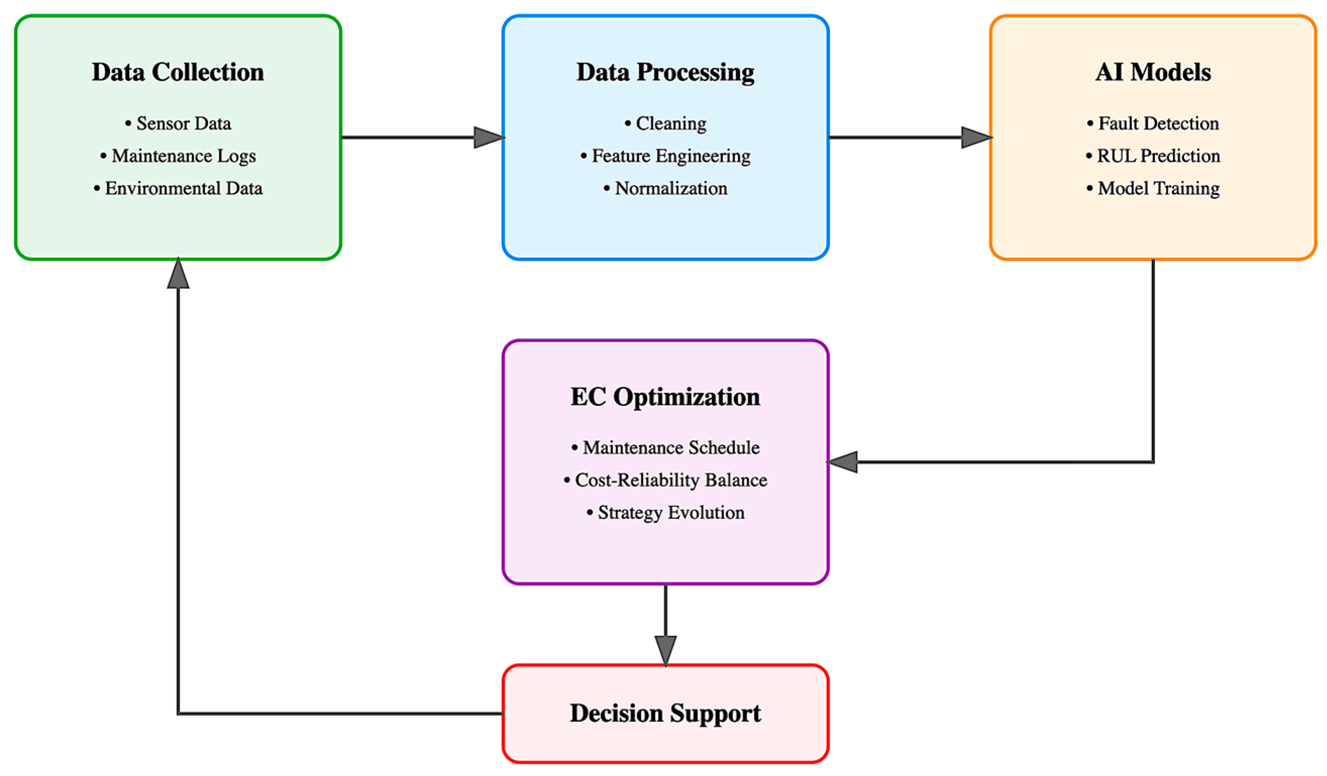
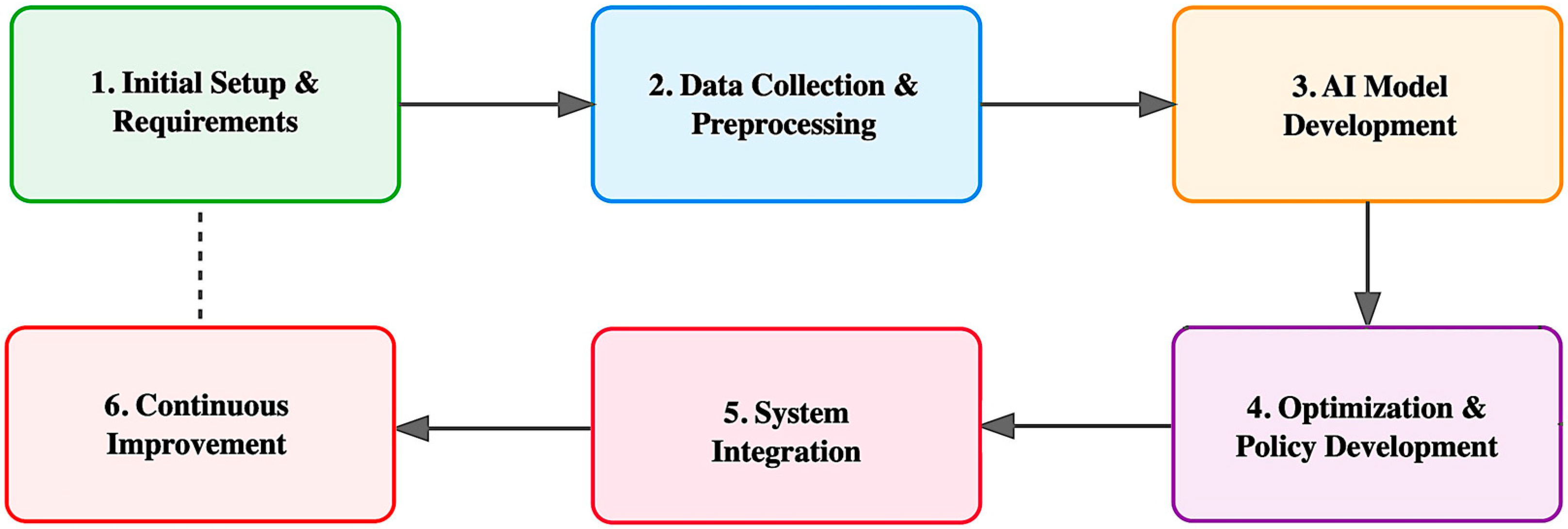
2.1. AI/EC Framework Development Methodology

The proposed AI/EC framework development methodology encompasses a comprehensive, multi-layered approach to create an integrated system for aircraft health monitoring and management. The framework consists of five essential layers: data processing, AI analysis, EC optimization, integration, and decision support, all working in concert to provide robust health monitoring capabilities (Figure 1).

The framework’s architecture implements a bidirectional flow where sensor data input progress through successive processing stages while maintaining continuous feedback loops for system optimization. The data processing layer serves as the foundation, incorporating sophisticated protocols for real-time sensor data acquisition and validation. A data flow management system ensures seamless integration between layers, maintaining data consistency, standardized protocols, and feedback mechanisms for adaptive system improvement.

The decision support layer synthesizes insights using a multi-level alert classification system and a maintenance recommendation engine that optimizes repair schedules based on cost–benefit analysis and resource availability. System validation involves comprehensive testing of prediction accuracy, false alarm rates, detection speed, and robustness against noise, missing data, and edge cases, ensuring technical reliability and operational feasibility.

While the proposed framework presents a structured methodology for fault detection and remaining useful life prediction, its application to AHM systems introduces specific adaptations that align with the unique challenges of aerospace operations. The specificity of the aerospace industry for the proposed approach is reflected in both the nature of the initial data and the methods used for their processing. Aircraft generate vast amounts of heterogeneous and high-frequency data from various subsystems, requiring specialized preprocessing techniques to ensure consistency, accuracy, and relevance for predictive modeling. The complexity of aerospace systems also necessitates the use of advanced AI and evolutionary computation techniques tailored to high-reliability environments. These methodological considerations, which form the core of this study, allow for the development of an adaptive and scalable framework that meets the stringent operational and safety requirements of aviation applications.

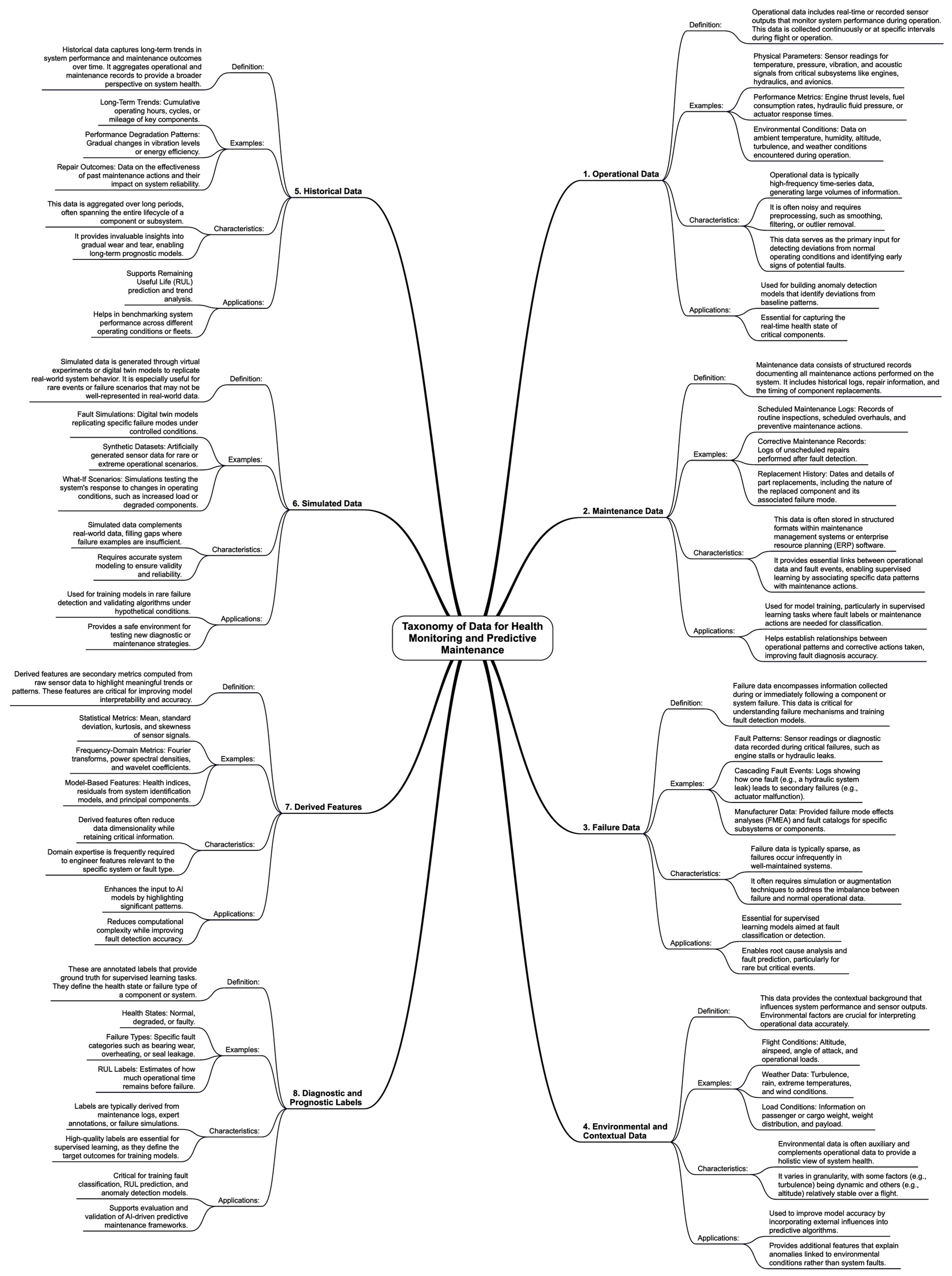
2.2. Data Collection

Data collection is a critical step in creating a robust framework for health monitoring and predictive maintenance. In the context of complex technical systems like aircraft, this process involves gathering operational data from multiple subsystems, each equipped with a variety of sensors that track parameters such as temperature, pressure, vibration, and acoustic signals. Additional data sources include flight logs, maintenance records, and contextual information on environmental or operating conditions (e.g., weather and load variations).

The focus is on a large and diverse dataset that reflects both normal operating conditions and fault events. Collaboration with engineering teams or domain experts identifies sensors and data points most indicative of system health. Archival or historical data are included to provide insight into the progression of faults over time. Data standardization procedures, such as synchronization of different sensor sampling rates and handling of missing values, ensure that the final dataset remains reliable, consistent, and suitable for subsequent modeling and analysis.

In the context of health monitoring and predictive maintenance for complex technical systems such as aircraft, data play a pivotal role in enabling accurate fault detection, diagnostics, and prognostics.

The taxonomy categorizes the diverse types of data required for building a comprehensive and effective framework for health monitoring and predictive maintenance (

Table 1. Framework of taxonomy of data required for aircraft health monitoring and predictive maintenance.

Category	Examples	Key Characteristics
Operational Data	Temperature, vibration, pressure	High-frequency, large volume, time-series
Maintenance Data	Inspection logs, repair records	Structured, links operations to interventions
Failure Data	Fault patterns, cascading events	Sparse, crucial for fault detection and classification
Environmental Data	Weather, flight conditions	Auxiliary input, context-dependent granularity
Historical Data	Long-term trends, cumulative cycles	Enables trend analysis and RUL estimation
Simulated Data	Digital twin outputs, synthetic faults	Fills data gaps, controlled testing environment
Derived Features	Statistical and frequency-domain metrics	Domain-specific, enhances model accuracy
Diagnostic/Prognostic Labels	Health states, failure types, RUL labels	Annotated, essential for supervised learning

). Each category contributes unique value, collectively enabling data-driven decision-making for complex systems like aircraft.

The taxonomy at Figure 2 provides a detailed breakdown of the various data types, categorized by their source, nature, and application within predictive maintenance frameworks. Each type contributes uniquely to the development of robust, data-driven systems for managing operational health and ensuring system reliability.

2.3. Data Preprocessing

Data preprocessing is essential for transforming raw sensor data into a structured format suitable for analysis. Modern systems, such as aircraft, generate vast amounts of noisy, inconsistent, or incomplete data, requiring preprocessing to ensure reliability in predictive maintenance and fault detection.

Key steps include data cleaning, which removes outliers using z-score analysis and domain-specific thresholds, noise filtering via moving averages or wavelet denoising, and missing value imputation through statistical methods or k-nearest neighbors. Standardization and normalization ensure feature consistency, critical for machine learning models.

Feature extraction derives relevant statistical and frequency-domain features, while data transformation segments time-series data using sliding windows, applies feature scaling, and reduces dimensionality with principal component analysis. Label alignment synchronizes maintenance logs with sensor data, while data augmentation expands datasets when failure data are scarce.

Finally, data integration and synchronization unify multiple data sources with varying sampling rates. The processed data are then split into training, validation, and testing sets to enhance model generalization and prevent overfitting.

Let us describe the mathematical formulation of data processing, broken down into each stage.

Let the system consist of $m$ sensors, each generating time-series data. The raw data collected at time $t$ is represented as

$$\mathbf{x}\left(t\right)=x_1\left(t\right),x_2\left(t\right),\dots ,x_m\left(t\right)$$

(1)

where $x_i\left(t\right)$ is the reading from the $i$-th sensor at time $t$. Additionally, external factors such as environmental or contextual variables are captured as

$$\mathbf{c}\left(t\right)=c_1\left(t\right),c_2\left(t\right),\dots ,c_k\left(t\right)$$

(2)

where $c_j\left(t\right)$ represents contextual variables like weather, load, or flight conditions. The complete raw data vector is

$$\mathbf{z}\left(t\right)=\left[\begin{array}{c}\mathbf{x}\left(t\right)\\ \mathbf{c}\left(t\right)\end{array}\right]$$

(3)

Outliers are identified using thresholds or statistical methods:

$$x_i\left(t\right) \mathrm{is} \mathrm{an} \mathrm{outlier} \mathrm{if} \left|x_i\left(t\right)-{\mu }_i\right|>k·{\sigma }_i$$

(4)

where ${\mu }_i$ is the mean and ${\sigma }_i$ is the standard deviation of $x_i\left(t\right)$, and $k$ is a chosen threshold (e.g., $k=3$).

Noise in the time-series data is smoothed using a moving average or low-pass filter:

$${\widehat{x}}_i\left(t\right)={\displaystyle \frac{1}{w}}\sum _{j=t-w+1}^t{x}_i\left(j\right)$$

(5)

where $w$ is the window size. Alternatively, wavelet denoising can be applied

$${\widehat{x}}_i\left(t\right)=W^{-1}\left\{\mathcal{T}\left[W\left(x_i\left(t\right)\right)\right]\right\}$$

(6)

where $W$ and $W^{-1}$ are the wavelet transform and inverse wavelet transform, and $\mathcal{T}$ is a thresholding function.

Missing values in $\mathbf{x}\left(t\right)$ are imputed using interpolation

$${\widehat{x}}_i\left(t\right)={\displaystyle \frac{x_i\left(t-1\right)+x_i\left(t+1\right)}{2}}$$

(7)

or advanced techniques like $k$-nearest neighbors

$${\widehat{x}}_i\left(t\right)={\displaystyle \frac{1}{k}}\sum _{j=1}^k{x_i}^{\left(j\right)}$$

(8)

where ${x_i}^{\left(j\right)}$ are the $k$-nearest neighbors of $x_i$ in the feature space.

Sensor readings are standardized to have zero mean and unit variance

$${\tilde{x}}_i\left(t\right)={\displaystyle \frac{x_i\left(t-1\right)-{\mu }_i}{{\sigma }_i}}$$

(9)

where ${\mu }_i$ and ${\sigma }_i$ are the mean and standard deviation of $x_i\left(t\right)$, respectively.

Alternatively, values can be normalized to a range $[a,b]$

$${\tilde{x}}_i\left(t\right)=a+{\displaystyle \frac{{[x}_i\left(t\right)-\underset{i}{\min }{x}_i\left]\right(b-a)}{\underset{i}{\max }{x}_i-\underset{i}{\min }{x}_i}}$$

(10)

Statistical features are computed over a sliding window of size $w$:

$${\mu }_i={\displaystyle \frac{1}{w}}\sum _{j=t-w+1}^t{x}_i\left(j\right), {\sigma }_i^2={\displaystyle \frac{1}{w}}\sum _{j=t-w+1}^t{\left[x_i\left(j\right)-{\mu }_i\right]}^2$$

(11)

$${skewness}_i=\sum _{j=t-w+1}^t{\left[{\displaystyle \frac{x_i\left(j\right)-{\mu }_i}{{\sigma }_i}}\right]}^3, {kurtosis}_i={\displaystyle \frac{1}{w}}\sum _{j=t-w+1}^t{\left[{\displaystyle \frac{x_i\left(j\right)-{\mu }_i}{{\sigma }_i}}\right]}^4-3$$

(12)

Frequency components are extracted using the Fourier transform:

$$X_i\left(f\right)=\sum _{t=1}^N{x}_i\left(t\right)e^{-j2\pi ft}$$

(13)

where $f$ represents frequency. The power spectral density is then computed as

$$P_i\left(f\right)={\left|X_i\left(f\right)\right|}^2$$

(14)

Residuals from system identification models can be used as features

$$r_i\left(t\right)=x_i\left(t\right)-{\widehat{x}}_i\left(t\right)$$

(15)

Time-series data are segmented into overlapping windows of size $w$

$$\mathbf{X}\left(t\right)=\mathbf{x}\left(t\right),\mathbf{x}\left(t+1\right),\dots ,\mathbf{x}\left(t+w-1\right)$$

(16)

High-dimensional data are reduced using principal component analysis

$${\mathbf{z}}_i={\mathbf{W}}^{\mathrm{\top }}{\mathbf{x}}_i$$

(17)

where $\mathbf{W}$ contains the principal components; the “transpose” symbol ($\mathrm{\top })$ is used to denote the transpose of a matrix.

For supervised learning tasks, each sample is paired with a corresponding label

$$\left[\mathbf{x}\left(t\right),y\left(t\right)\right]$$

(18)

where $y\left(t\right)$ represents the health state (e.g., “normal” or “faulty”) or remaining useful life.

RUL labels are computed as

$$y\left(t\right)=T_{failure}-t.$$

(19)

where $T_{failure}$ is the known time of failure.

Simulated data are generated using a digital twin or system model

$$x_{sim}\left(t\right)=F\left[\mathbf{s}\left(t\right),\mathbf{u}\left(t\right),\mathbf{w}\left(t\right)\right]$$

(20)

where $F$ is the system dynamics function, $\mathbf{s}\left(t\right)$ is the system state, $\mathbf{u}\left(t\right)$ are inputs, and $\mathbf{w}\left(t\right)$ represents noise.

Data streams with different sampling rates are resampled to a common frequency $f_c$

$${\mathbf{x}}_i^{resampled}\left(t\right)={\mathbf{x}}_i\left(t{\displaystyle \frac{f_i}{f_c}}\right)$$

(21)

where $f_i$ is the original sampling rate of the $i$-th sensor.

The final processed dataset is divided into training, validation, and testing subsets

$$Dataset=\left\{{\mathbf{X}}_{train},{\mathbf{X}}_{val},{\mathbf{X}}_{test}\right\}$$

(22)

where ${\mathbf{X}}_{train}$ is used for model training, ${\mathbf{X}}_{val}$ is used for hyperparameter tuning, and ${\mathbf{X}}_{test}$ is reserved for evaluating model performance.

By following these preprocessing steps, raw sensor data are transformed into a high-quality, consistent dataset that supports the development of reliable and accurate AI-driven models for fault detection, diagnosis, and predictive maintenance. This comprehensive approach ensures the effective utilization of data in managing the health of complex technical systems such as aircraft.

2.4. Feature Engineering and Selection

To ensure the effectiveness of fault detection and RUL prediction, the framework extracts a diverse set of features from sensor data, aligning with best practices in AHM. As illustrated in Figure 2, the extracted data originate from multiple sources, including operational, maintenance, failure, environmental, historical, and simulated data. These features are categorized into time-domain, frequency-domain, and domain-specific engineered features to maximize predictive accuracy.

Time-domain features capture statistical patterns in sensor readings, including mean, variance, skewness, kurtosis, root mean square, peak-to-peak values, and temporal gradients to assess the rate of degradation. Frequency-domain features use fast Fourier transform, wavelet transform coefficients, power spectral density, and energy of specific frequency bands to identify spectral components associated with fault signatures. Domain-specific features integrate health indices from sensor fusion models, residual-based deviations from physics-informed models, and trend-based features from RUL estimation models, ensuring comprehensive degradation analysis.

Feature engineering and selection transform raw sensor data into meaningful inputs for machine learning, improving model performance, reducing complexity, and enhancing interpretability—especially in high-volume, multi-sensor environments like aircraft systems. Dimensionality reduction methods refine high-dimensional data while preserving critical information.

Relevant studies have demonstrated the effectiveness of these approaches in AHM applications [84], supporting the transition toward data-driven feature engineering rather than relying solely on manually engineered descriptors. This evolution enhances system efficiency and fault prediction accuracy, aligning with modern trends in AI-powered aviation maintenance solutions.

Wavelet transforms can also be used to extract localized frequency components:

$$W_i\left(\tau ,s\right)={\int }_{-\infty }^{\infty }{x}_i\left(t\right){\psi }^{*}\left({\displaystyle \frac{t-\tau }{s}}\right)dt$$

(23)

where symbol $s$ represents the scale parameter in the wavelet transform; symbol (*) denotes the complex conjugate of the oscillatory function $\psi$ used to analyze the signal. The wavelet transforms produce $W_i\left(\tau ,s\right)$, which represents the correlation between the signal $x_i\left(t\right)$) and the wavelet $\psi$ at a specific time $\tau$ and scale $s$. This provides a time-frequency representation of the signal, useful for identifying features like trends, discontinuities, or oscillatory patterns.

Custom features are derived using expert knowledge. For instance, residuals from a model $r_i=x_i\left(t\right)-{\widehat{x}}_i\left(t\right)$ and vibration signatures $v_i={\underset{f\in \mathcal{F}}{\max }P}_i(f)$, where $\mathcal{F}$ is a set of fault-specific frequencies.

Let the feature vector after engineering be

$$\mathbf{z}\left(t\right)=z_1\left(t\right),z_2\left(t\right),\dots ,z_d\left(t\right)$$

(24)

where $d$ is the number of engineered features.

A binary selection vector $\mathsf{\alpha }={\alpha }_1,{\alpha }_2,\dots ,{\alpha }_d$ is introduced, where

$${\alpha }_i=\left\{\begin{array}{cc}1\hfill & \hfill \mathrm{i}\mathrm{f} \mathrm{f}\mathrm{e}\mathrm{a}\mathrm{t}\mathrm{u}\mathrm{r}\mathrm{e} z_i \mathrm{i}\mathrm{s} \mathrm{s}\mathrm{e}\mathrm{l}\mathrm{e}\mathrm{c}\mathrm{t}\mathrm{e}\mathrm{d}\\ 0\hfill & \hfill \mathrm{i}\mathrm{f} \mathrm{f}\mathrm{e}\mathrm{a}\mathrm{t}\mathrm{u}\mathrm{r}\mathrm{e} z_i \mathrm{i}\mathrm{s} \mathrm{e}\mathrm{x}\mathrm{s}\mathrm{e}\mathrm{l}\mathrm{e}\mathrm{c}\mathrm{t}\mathrm{e}\mathrm{d}\end{array}\right.$$

(25)

The selected feature set is

$$z_{\alpha }\left(t\right)=\left[z_i\left(t\right):{\alpha }_i=1\right]$$

(26)

Feature selection aims to maximize the performance of a predictive model while minimizing the number of selected features. The objective function is

$$\underset{\alpha }{\min }\mathcal{J}\left(\mathsf{\alpha }\right)=-Acc\left[{\mathbf{z}}_{\alpha }\left(t\right)\right]+\lambda ‖\mathsf{\alpha }‖$$

(27)

where $Ass(·)$ is the model accuracy, $‖\mathsf{\alpha }‖={\sum }_{i=1}^d{\alpha }_i$ is the number of selected features, and $\lambda$ is a penalty coefficient balancing accuracy and feature sparsity.

Using evolutionary algorithms, feature selection is treated as a combinatorial optimization problem. A population of binary vectors $\{{\mathsf{\alpha }}_1,{\mathsf{\alpha }}_2,\dots ,{\mathsf{\alpha }}_N\}$ evolved over generations. The fitness of each individual ${\mathsf{\alpha }}_i$ is evaluated using the objective function $\mathcal{J}\left({\mathsf{\alpha }}_i\right)$.

Genetic operators, such as crossover and mutation, are applied to explore the feature space: crossover combines two parent feature subsets to produce offspring, mutation randomly flips bits in ${\mathsf{\alpha }}_i$ to introduce diversity.

Over successive iterations, the algorithm converges to an optimal or near-optimal feature subset.

The final feature set ${\mathbf{z}}_{\alpha }\left(t\right)$ is used to train the machine learning model

$$\widehat{y}\left(t\right)=f\left[{\mathbf{z}}_{\alpha }\left(t\right);\mathit{\theta }\right]$$

(28)

where $f$ is the predictive model parameterized by $\mathit{\theta }$; $\widehat{y}\left(t\right)$ is the predicted output (e.g., fault type or remaining useful life).

This mathematical framework captures the key aspects of feature engineering and selection, starting from raw sensor data, extracting informative features, reducing dimensionality, and optimizing feature subsets for predictive model development.

2.5. Differentiation Between Fault Detection and Remaining Useful Life Prediction

Fault detection and remaining useful life prediction are two distinct but complementary tasks in aviation health monitoring, each requiring specialized AI methodologies due to fundamental differences in their objectives and data structures.

• Fault Detection as a Classification/Anomaly Detection Task

Fault detection aims to identify abnormal system behavior by distinguishing between normal and faulty conditions. This is typically framed as a classification or anomaly detection problem, where the model detects deviations from expected operational patterns. Common AI-based fault detection approaches include

• Supervised learning (e.g., random forest, support vector machines, neural networks) requires labeled historical fault data to train a classifier capable of distinguishing failure modes.
• Clustering (e.g., K-Means, DBSCAN) identifies anomalies by grouping similar operational patterns and flagging outliers as potential faults.
• Autoencoder-based anomaly detection learns a compressed representation of normal behavior and detects faults when reconstruction errors exceed a predefined threshold.

The proposed framework employs a random forest classifier, optimized through a genetic algorithm for feature selection and hyperparameter tuning. This combination improves fault detection accuracy by leveraging both ensembles’ learning robustness and evolutionary optimization for adaptive learning.

2.

RUL Prediction as a Regression-Based Temporal Forecasting Task

In contrast to fault detection, RUL prediction involves estimating the remaining time before system failure by modeling temporal degradation trends. Since the target variable (remaining life) is continuous, RUL prediction is treated as a regression problem, requiring models capable of capturing time-dependent patterns. Common techniques include

• Recurrent neural networks (RNNs) and long short-term memory (LSTM) networks—well-suited for sequential data modeling, learning from historical degradation patterns to predict future failure points.
• Kalman filters are state-space models that provide real-time updates on system health based on sensor data.
• Survival analysis (e.g., Weibull distribution models) estimates the probability of failure over time based on operational history.

In the proposed framework, a random forest regressor is used for RUL estimation, using feature importance analysis for better interpretability. The choice of random forest over deep learning architectures (e.g., LSTM) is justified by the limited size of labeled degradation data in aviation maintenance, where deep networks may struggle with overfitting.

3.

Integration of Fault Detection and RUL Prediction in the Proposed Framework

Fault detection and RUL prediction are integrated within a unified decision-making framework, where

• The fault detection model first identifies system anomalies. If a fault is detected, the system transitions to predictive maintenance mode.
• The RUL prediction model estimates the time remaining before failure, allowing for proactive maintenance scheduling.
• The two models share extracted feature representations, ensuring consistency between classification-based fault identification and regression-based lifespan estimation.

By incorporating both techniques, the proposed system enables real-time fault detection while providing long-term predictive insights, enhancing aviation safety and maintenance efficiency.

2.6. AI Model Development

AI model development is key to fault detection, anomaly classification, and remaining useful life prediction in aviation health monitoring. It involves selecting, training, and validating models to ensure reliability and adaptability.

Model selection depends on the task: supervised learning models handle classification, while unsupervised models detect anomalies without labeled data. Time-series models predict RUL using sequential sensor data.

Training involves defining loss functions, tuning hyperparameters, and applying regularization techniques to prevent overfitting. Evaluation metrics include accuracy, precision, recall, and F1-score for classification, and RMSE and R² for regression. Cross-validation ensures unbiased performance estimates.

To address imbalanced datasets, the SMOTE technique helps to balance normal and fault conditions. Data augmentation, using digital twins or simulations, improves model robustness, ensuring high-performance predictive maintenance in aviation systems.

After successful validation, the trained model is deployed for real-time monitoring and predictive maintenance. In real-time applications, the model continuously updates predictions as new sensor data become available. Retraining with new data ensures that the model adapts to evolving operating conditions or previously unseen faults. To improve usability and trust, explainability techniques such as SHapley Additive exPlanations (SHAP) [85] or Local Interpretable Model-agnostic Explanations (LIME) [86] provide insights into the model’s decisions, aiding engineers in understanding and utilizing the model effectively.

The mathematical formulation of AI model development encompasses the selection, training, evaluation, and deployment of models for fault detection, anomaly identification, and remaining useful life prediction.

For classification or regression tasks, supervised models aim to learn a function $f$ parameterized by $\mathit{\theta }$

$${\widehat{y}}_i=f\left({\mathbf{z}}_i;\mathit{\theta }\right)$$

(29)

where $f$ is the model (e.g., neural network, support vector machines, random forest); $\mathit{\theta }$ is the model parameters (e.g., weights in a neural network).

Unsupervised models identify anomalies by modeling the distribution of normal data. For example, an autoencoder minimizes the reconstruction error

$${\mathcal{L}}_{recon}={\displaystyle \frac{1}{n}}\sum _{i=1}^n{‖{\mathbf{z}}_i-g\left[h\right({\mathbf{z}}_i;\varphi ;\psi \left)\right]‖}^2$$

(30)

where $h({\mathbf{z}}_i;\varphi ;\psi )$ is the encoder function; $g$ is the decoder function.

For RUL prediction, time-series models (e.g., long-short term models) predict future values

$${\widehat{y}}_i=f[\left({\mathbf{z}}_i\left(t\right),{\mathbf{z}}_i\left(t-1\right),\dots ,{\mathbf{z}}_i\left(t-k\right);\mathit{\theta }\right]$$

(31)

where $k$ is the size of the time window.

The choice of loss function depends on the task:

• Classification loss (cross-entropy)

$${\mathcal{L}}_{CE}=-{\displaystyle \frac{1}{n}}\sum _{i=1}^n\sum _{j=1}^C{y}_{ij}\log \left(y_{ij}\right)$$

(32)

where $C$ is is the number of classes, $y_{ij}$ is a binary indicator for the true class, and ${\widehat{y}}_{ij}$ is the predicted probability.

• Regression loss (mean squared error)

$${\mathcal{L}}_{MSE}={\displaystyle \frac{1}{n}}\sum _{i=1}^n{(y_i-y_{ij})}^2$$

(33)

• Anomaly detection loss (reconstruction error)

$${\mathcal{L}}_{recon}={\displaystyle \frac{1}{n}}\sum _{i=1}^n{‖{\mathbf{z}}_i-{\widehat{\mathbf{z}}}_i‖}^2$$

(34)

Model parameters $\mathit{\theta }$ are optimized using gradient-based methods

$${\mathit{\theta }}^{*}=\mathrm{a}\mathrm{r}\mathrm{g} \underset{\mathit{\theta }}{\min }\mathcal{L}(\mathit{\theta })$$

(35)

where $\mathcal{L}$ represents the chosen loss function. Optimization algorithms like stochastic gradient descent [87] or Adam [88] are used.

To prevent overfitting, regularization techniques are applied:

$${\mathcal{L}}_{reg}=\mathcal{L}+\lambda {‖\mathit{\theta }‖}^2$$

(36)

where $\lambda$ controls the penalty strength.

The model is evaluated using appropriate metrics for the task:

• Classification metrics

$$Accuracy={\displaystyle \frac{Number of Correct Predictions}{Total Predictions}}$$

(37)

$$Precission={\displaystyle \frac{True Positives}{True Positives+False Positives}}$$

(38)

$$Recall={\displaystyle \frac{True Positives}{True Positives+False Negatives}}$$

(39)

$$F1 Score=2·{\displaystyle \frac{Precission ·Recall}{Precission+Recall}}$$

(40)

• Regression metrics

$$RNSE=\sqrt{{\displaystyle \frac{1}{n}}\sum _{i=1}^n({y_i-{\widehat{y}}_i)}^2}$$

(41)

$$R^2=1-{\displaystyle \frac{{\sum }_{i=1}^n({y_i-{\widehat{y}}_i)}^2}{{\sum }_{i=1}^n{\left(y_i-\overline{y}\right)}^2}}$$

(42)

• Anomaly detection metrics

Precision-recall area under the curve or receiver operating characteristic area under the curve assesses the quality of anomaly detection. Both metrics assess how effectively the anomaly detection model separates anomalous events from normal observations.

For imbalanced datasets, additional techniques can be applied:

• Class weights which modify the loss function to assign higher weights to minority classes

$${\mathcal{L}}_{weighted}={\displaystyle \frac{1}{n}}\sum _{i=1}^n{w}_{y_i}\log \left({\widehat{y}}_i\right)$$

(43)

where $w_{y_i}$ is the weight for class $y_i$.

• Data augmentation which generates synthetic samples using methods like SMOTE

$${\mathbf{z}}_{new}={\mathbf{z}}_i+\alpha \left({\mathbf{z}}_{\mathbf{j}}-{\mathbf{z}}_i\right)$$

(44)

where $\alpha$ is a scalar value drawn randomly from a uniform distribution $U\left(\mathrm{0,1}\right)$.

In real-time deployment, the model processes streaming data $\mathbf{z}\left(t\right)$ to provide continuous predictions

$$\widehat{y}\left(t\right)=f\left[\mathbf{z}\left(t\right);\mathit{\theta }\right]$$

(45)

where the predictions are integrated into maintenance decision systems.

Model retraining incorporates new data

$${\mathit{\theta }}_{new}=\arg \underset{\mathit{\theta }}{\min }{\mathcal{L}}_{updated}(\mathit{\theta })$$

(46)

where ${\mathcal{L}}_{updated}$ includes the latest data.

This mathematical framework formalizes AI model development for fault detection, anomaly identification, and RUL prediction. It covers input data representation, loss functions, optimization, evaluation metrics, and real-time deployment, providing a structured approach to developing robust and adaptive models for predictive maintenance in complex systems.

2.7. Multi-Objective Optimization and Predictive Maintenance

Existing studies in AHM primarily focus on either fault detection or RUL prediction as standalone tasks, with limited integration of both within a unified AI-driven optimization framework. While previous research has successfully applied machine learning and deep learning models to specific aircraft components such as engines, hydraulic systems, and avionics, challenges remain in multi-source sensor fusion, real-time adaptive learning, and computational efficiency for onboard deployment.

Furthermore, predictive maintenance strategies in aviation still rely heavily on rule-based decision-making or predefined thresholding methods, limiting their ability to adapt to dynamic operational conditions. The application of evolutionary optimization techniques for fault classification refinement, feature selection, and maintenance scheduling remains underexplored, particularly in scenarios requiring real-time decision support.

Multi-objective optimization is a key component of an effective framework for managing the health of complex technical systems. It focuses on balancing competing objectives such as maximizing safety, minimizing operational costs, and reducing downtime, while ensuring the system operates reliably. In aircraft maintenance, this involves optimizing fault detection, repair schedules, and resource allocation to achieve long-term efficiency and safety goals.

The maintenance decision-making process often involves trade-offs among conflicting objectives. For example, replacing a component prematurely increases maintenance costs but reduces the risk of failure. Conversely, extending the operational life of a component may decrease immediate costs but increases the likelihood of unexpected failures. Multi-objective optimization provides a structured approach to balance these trade-offs by optimizing a set of objective functions simultaneously.

A typical multi-objective optimization problem in predictive maintenance is formulated as

• Reducing the costs of inspections, repairs, and replacements.
• Ensuring the system remains operational for as long as possible.
• Reducing the probability of critical failures by addressing faults proactively.

Solutions to these problems are evaluated using Pareto efficiency, where no single solution is superior in all objectives. A Pareto front is constructed, representing a set of optimal trade-offs among competing objectives. Maintenance planners can then select the most appropriate solution based on priorities such as cost, risk tolerance, or operational needs.

Predictive maintenance uses real-time and historical data to predict when a component is likely to fail and schedule maintenance at the optimal time. This approach integrates machine learning models, statistical methods, and optimization algorithms to determine RUL and recommend maintenance actions before critical failures occur.

Key steps in predictive maintenance include

• Identifying potential faults early using anomaly detection models or classification algorithms.
• Estimating the RUL of components based on sensor data, operational conditions, and historical trends.
• Optimizing when and how maintenance actions are performed to minimize costs and downtime while maintaining reliability.

Predictive maintenance incorporates both short-term and long-term planning. Short-term decisions involve responding to immediate risks, such as replacing a component with low RUL. Long-term strategies focus on optimizing resource allocation, inventory management, and fleet-wide maintenance schedules.

Optimization algorithms, particularly multi-objective evolutionary algorithms (e.g., NSGA-II [89], MOEA/D [90]), are well-suited for addressing the complexities of predictive maintenance. These algorithms simulate a population of potential solutions, where each solution represents a maintenance strategy. Over successive generations, the solutions evolve, balancing objectives like cost, downtime, and reliability. Key components include

• Representing maintenance decisions, such as repair schedules or thresholds for fault intervention.
• Assessing the quality of each solution based on the objectives.
• Applying crossover and mutation to generate diverse solutions and explore the solution space.

The results of multi-objective optimization and predictive maintenance models are integrated into actionable maintenance policies. These policies define thresholds for fault intervention, prioritize maintenance tasks, and allocate resources dynamically based on system health and operational constraints. For instance, if a component’s RUL falls below a predefined threshold, the policy triggers a maintenance action, balancing cost and safety considerations.

Modern predictive maintenance frameworks incorporate real-time data streams to adapt maintenance policies dynamically. For example, updated sensor readings can refine RUL predictions and trigger maintenance actions sooner if the risk of failure increases. Adaptive models ensure that maintenance decisions remain optimal as system conditions evolve.

Multi-objective optimization and predictive maintenance involve mathematical frameworks that balance competing goals, such as minimizing costs, reducing downtime, and maximizing reliability. Below is the formalization of these processes.

Multi-objective optimization and predictive maintenance involve mathematical frameworks that balance competing goals, such as minimizing costs, reducing downtime, and maximizing reliability.

A general multi-objective optimization problem can be expressed as

$$\underset{u}{\min }\mathbf{J}\left(\mathbf{u}\right)=\left[\begin{array}{c}{J}_1\left(\mathbf{u}\right)\\ \begin{array}{c}{J}_2\left(\mathbf{u}\right)\\ \dots \end{array}\\ J_k\left(\mathbf{u}\right)\end{array}\right]$$

(47)

where $\mathbf{u}$ is the decision vector (e.g., maintenance actions, schedules, or thresholds), $\mathbf{J}\left(\mathbf{u}\right)$ is a vector of $k$ objective functions representing competing goals; for example, maintenance cost (e.g., cost of repairs, replacements, inspections), downtime (e.g., operational hours lost due to maintenance), reliability (e.g., probability of avoiding failures or maximizing system health) and others.

Constraints are imposed to ensure feasible solutions

$$g_i\left(\mathbf{u}\right)\le 0, i=1,\dots ,n$$

(48)

$$h_j\left(\mathbf{u}\right)=0, j=1,\dots ,m$$

(49)

where $g_i$ are inequality constraints (e.g., budget limits or safety thresholds) and $h_j$ are equality constraints (e.g., operational constraints).

Predictive maintenance uses system health data to schedule maintenance actions.

The RUL of a component is predicted using a machine learning or statistical model:

$${\widehat{RUL}}_i=f\left({\mathbf{z}}_i;\mathit{\theta }\right)$$

(50)

where ${\mathbf{z}}_i$ is the feature vector for the $i$-th component, $\mathit{\theta }$ are model parameters, and ${\widehat{RUL}}_i$ is predicted time before failure.

Maintenance actions $\mathbf{u}$ are represented as a vector

$$\mathbf{u}=\left[u_1,u_2,\dots ,u_n\right]$$

(51)

where $u_i\in \{\mathrm{0,1},2\}$ indicates the type of maintenance action: $u_i=0$ no action, $u_i=1$ minor repair, $u_i=2$ component replacement.

Maintenance schedules aim to minimize costs while ensuring reliability. The total cost $C_{total}$ over a planning horizon $T$ can be expressed as

$$C_{total}=\sum _{t=1}^T\{C_m[\mathbf{u}(t)]+C_f[\mathbf{s}(t)]\}$$

(52)

where $C_m\left[\mathbf{u}\right(t\left)\right]$ is cost of maintenance actions at time $t$, $C_f\left[\mathbf{s}\right(t\left)\right]$ is expected failure cost based on system state $\mathbf{s}\left(t\right)$.

The following objective functions can be used:

• Maintenance cost

$$J_1\left(\mathbf{u}\right)=\sum _{t=1}^T{C}_m\left[\mathbf{u}\left(t\right)\right]$$

(53)

where $C_m\left[\mathbf{u}\right(t\left)\right]$ includes labor, parts, and operational costs associated with each action.

• System downtime

$$J_2\left(\mathbf{u}\right)=\sum _{t=1}^{T}D\left[\mathbf{u}\right(t\left)\right]$$

(54)

where $D\left[\mathbf{u}\right(t\left)\right]$ is the downtime caused by maintenance actions at time $t$.

• Reliability maximization

$$J_3\left(\mathbf{u}\right)=\sum _{t=1}^T[1-R(t\left)\right]$$

(55)

where $[1-R\left(t\right)]$ ensures reliability maximization.

Multi-objective optimization can be realized with evolutionary algorithms:

• Pareto optimization. The solution to the multi-objective optimization problem is a Pareto front

$$\mathcal{P}=\left\{{\mathbf{u}}^{*}:\nexists \mathbf{u} \mathrm{s}\mathrm{u}\mathrm{c}\mathrm{h} \mathrm{t}\mathrm{h}\mathrm{a}\mathrm{t} J_i\left({\mathbf{u}}^{*}\right)|\forall i\right\}$$

(56)

A Pareto-optimal solution improves one objective without degrading another.

• Evolutionary algorithm implementation:

  o

  Solutions $\mathbf{u}$ are represented as chromosomes.

  o

  A population of solutions is generated.

  o

  Each solution is evaluated using

  $$\mathbf{J}\left(\mathbf{u}\right)=\left[J_1\left(\mathbf{u}\right),J_2\left(\mathbf{u}\right),J_3\left(\mathbf{u}\right)\right]$$

  (57)

  o

  Crossover and mutation introduce diversity.

  o

  Non-dominated solutions are selected to form the next generation.

Predictive maintenance integration has the next steps.

As new sensor data $\mathbf{z}\left(t\right)$ become available, RUL predictions are updated

$${\widehat{RUL}}_i=f\left({\mathbf{z}}_i;\mathit{\theta }\right)$$

(58)

Maintenance decisions are dynamically adjusted

$$\mathbf{u}\left(t\right)=\pi \left[\widehat{RUL}\left(t\right),\mathbf{s}\left(t\right)\right]$$

(59)

where $\pi$ is a policy derived from the optimization framework.

The optimal maintenance policy ${\pi }^{*}$ minimizes the total cost while satisfying reliability constraints:

$${\pi }^{*}=\arg \underset{\pi }{\min }\sum _{t=1}^T\{C_m[\pi (t)]+C_f[\mathbf{s}(t)]\}$$

(60)

subject to $R\left(t\right)\ge R_{min}, \forall t$.

This mathematical framework formalizes multi-objective optimization and predictive maintenance by defining objective functions, constraints, and optimization algorithms. It balances competing goals such as cost, downtime, and reliability, using tools like evolutionary algorithms to derive optimal maintenance policies. Real-time adaptation ensures that the framework remains effective as system conditions evolve, making it well-suited for managing the health of complex technical systems like aircraft.

3. Results

3.1. System Integration and Architecture

System integration and architecture form the backbone of a robust framework for health monitoring and predictive maintenance in complex technical systems like aircraft. This framework integrates data collection, processing, model inference, optimization algorithms, and decision-making systems into a cohesive structure that operates in real time, adapts to evolving conditions, and supports proactive maintenance actions. The design prioritizes modularity, scalability, and robustness to address the complexities of modern systems.

The architecture is organized into modular components, each responsible for specific functions and interconnected through well-defined interfaces. The key modules include a data acquisition and storage module that collects raw sensor data, maintenance logs, and contextual information from onboard systems, IoT devices, and databases, storing these data in centralized or distributed repositories. The data processing module cleans, preprocesses, and engineers features, transforming raw data into formats suitable for analysis. The AI model inference module applies trained models for fault detection, classification, anomaly detection, and RUL prediction. An optimization engine executes multi-objective optimization algorithms to derive optimal maintenance schedules and actions, while a decision-making interface provides actionable insights, including alerts, recommendations, and scheduling outputs, to engineers or automated systems.

The architecture ensures efficient data flow across modules through communication pipelines. Real-time sensor data streams are routed to the data processing module for immediate transformation and analysis, and the processed features are passed to the AI model inference module for generating predictions, such as fault probabilities or RUL estimates. These predictions feed into the optimization engine, which integrates them with maintenance policies and operational constraints to compute optimal actions. The decision-making interface communicates these recommendations and alerts to operators, enabling timely and informed maintenance decisions.

The system supports both real-time and batch processing. Real-time processing is critical for tasks like fault detection and RUL prediction, where sensor data streams must be continuously analyzed to provide immediate alerts or decisions. Batch processing, on the other hand, is used for periodic optimization of maintenance schedules, retraining models with updated data, or conducting detailed analyses of historical data.

The architecture can be implemented as either a centralized or distributed system.

In a centralized architecture, all data processing, model inference, and optimization are performed in a central system, typically cloud-based, ensuring easy scalability and central management, though with potential latency in real-time scenarios (Figure 3).

The centralized architecture for AHM and management systems is a structured approach in which all data collection, processing, model inference, and decision-making occur within a unified computational environment, typically a cloud-based or centralized server infrastructure. This system integrates data from multiple aircraft, consolidating it into a central repository where advanced analytics and AI-driven predictive models are applied.

In this architecture, sensor data from various onboard aircraft systems—including engines, avionics, hydraulics, and structural components—is continuously transmitted to a central processing unit. The centralized computational hub performs real-time fault detection, predictive maintenance analysis, and multi-objective optimization for maintenance decision-making. AI models are trained and deployed centrally, ensuring consistency across all aircraft in the fleet.

One of the key advantages of a centralized AHM system is the ability to use high computational power for large-scale data analytics and deep learning model training. Since all aircraft data are stored in a unified database, pattern recognition and anomaly detection benefit from an extensive historical dataset, improving model accuracy over time. Additionally, centralized systems provide standardized maintenance decision support, ensuring that operational insights and recommendations are uniformly applied across different fleet units.

However, a major challenge of this architecture is the potential for latency in real-time applications due to network transmission delays, particularly in remote or high-altitude conditions where connectivity might be unstable. This latency can impact critical decision-making processes, such as real-time anomaly detection or urgent maintenance alerts. Furthermore, reliance on a single central system introduces a single point of failure, necessitating robust redundancy and cybersecurity measures to ensure system resilience.

Despite these challenges, the centralized AHM system remains a preferred solution for large-scale fleet management, enabling high data integrity, centralized model updates, and efficient resource allocation for predictive maintenance operations.

In a distributed architecture, processing tasks are decentralized across edge devices, onboard systems, and cloud infrastructure, reducing latency for real-time decisions and enhancing resilience for aircraft operating in remote conditions (Figure 4).

The distributed architecture for AHM and management systems decentralizes data processing, enabling real-time decision-making closer to the data source. Unlike a centralized system that relies on a single computational hub, the distributed approach distributes computing tasks across multiple processing layers, including onboard aircraft systems, edge devices, and cloud infrastructure.

In this architecture, aircraft sensors continuously generate data related to engine performance, avionics, structural health, and environmental conditions. Instead of transmitting all raw data to a central server, onboard processing units and edge computing devices analyze data locally. These localized computations enable real-time fault detection, anomaly classification, and predictive maintenance estimations without excessive reliance on external network connectivity.

The key advantage of a distributed system is its low-latency response, which is crucial for safety-critical applications in aviation. Since fault detection and predictive analytics occur at multiple levels, immediate alerts can be generated onboard when sensor readings indicate abnormal conditions. Additionally, only processed and essential data are transmitted to the cloud, significantly reducing bandwidth usage and network load while maintaining comprehensive historical records for fleet-wide maintenance analysis.

Furthermore, a distributed AHM system enhances operational resilience by reducing dependency on a single point of failure. If a network outage occurs, local processing units continue to function autonomously, ensuring that maintenance recommendations and safety alerts remain accessible. The system can also adapt dynamically to varying operational environments, adjusting data processing strategies based on available computational resources and network conditions.

However, implementing a distributed architecture introduces challenges in system coordination and integration. Synchronization between onboard, edge, and cloud systems is critical to ensure consistency in maintenance decisions across the fleet. Additionally, the computational limitations of edge devices may restrict the complexity of AI models that can be deployed locally, requiring an optimized balance between onboard and cloud-based analytics.

Integration with existing systems ensures seamless functionality. The framework interfaces with AHM systems as data sources or feedback mechanisms and with maintenance management systems to automate workflows and streamline operations. IoT-enabled devices further enhance data collection and communication for efficient monitoring.

The design emphasizes adaptability and scalability to meet evolving operational requirements. AI models are retrained periodically, or dynamically as new data become available, ensuring continuous improvement in predictive accuracy. The modular architecture supports the addition of new sensors, subsystems, or aircraft without significant reconfiguration, and fault-tolerant design ensures system resilience during hardware or communication failures.

A user-friendly interface enhances accessibility and usability by presenting actionable insights through real-time dashboards that display system health, fault probabilities, and RUL estimates. The system includes an alert mechanism for imminent faults or maintenance needs, highlighting critical components and suggested actions. Historical analysis tools allow users to explore trends, fault progression, and the outcomes of past maintenance actions, enabling data-driven decision-making.

To ensure the security and confidentiality of data, the system incorporates encryption for data transmission and storage, access controls to restrict sensitive data and decision-making modules, and compliance with industry regulations and standards governing data privacy and aviation safety.

This integrated and modular architecture supports proactive, data-driven maintenance strategies, enhancing reliability, reducing costs, and improving operational efficiency for complex technical systems like aircraft. Its scalability, adaptability, and resilience make it suitable for dynamic environments and long-term applications.

3.2. Dataset Characteristics and Feature Selection

A well-structured dataset is essential for building robust fault detection and remaining useful life prediction models. This section presents a detailed overview of the extracted and selected features, the dataset split strategy, and an analysis of feature distributions.

• Number of Extracted Features (Numerical and Categorical)

In our feature engineering process, we extracted a total of 48 numerical features and three categorical features from the sensor data. These features were derived from multiple sensor channels monitoring parameters such as temperature, pressure, and vibration.

• Numerical features (48 total):

  o

  Time-domain statistical features (18 features): Mean, variance, standard deviation, skewness, kurtosis, root mean square (RMS), peak-to-peak amplitude, signal energy, entropy, interquartile range, crest factor, shape factor, impulse factor, margin factor, slope, zero-crossing rate, range, and median absolute deviation.

  o

  Frequency-domain features (12 features): Fourier-transform coefficients, dominant frequency component, spectral entropy, power spectral density in selected frequency bands, wavelet decomposition coefficients.

  o

  Domain-specific features (18 features): Residual error from a degradation model, moving average trend deviation, slope of feature degradation, cumulative damage index, trend-based anomaly detection scores, and autoregressive model parameters.

• Categorical features (three total). These represent operating states of the system (normal, warning, faulty), encoded using one-hot encoding for integration with machine learning models.

These extracted features serve as the input for fault detection and RUL prediction models.

2.

Number of Selected Features

To optimize model performance while reducing computational complexity, we applied feature selection using a combination of genetic algorithms and feature importance analysis from the trained Random Forest model. This process selected 22 features from the original 51 extracted features.

• Selected Numerical Features (19 total):

  o

  Time-domain statistical features (eight features): Mean, standard deviation, root mean square (RMS), skewness, kurtosis, peak-to-peak amplitude, entropy, and zero-crossing rate.

  o

  Frequency-domain features (six features): Dominant frequency component, spectral entropy, power spectral density in low and mid-frequency bands, wavelet transform coefficient at level 3, and spectral centroid.

  o

  Domain-specific features (five features): Cumulative damage index, residual error from degradation model, moving average trend deviation, trend-based anomaly detection score, and autoregressive model parameter.

• Selected Categorical Features (three total). These represent the system’s operational condition (normal, warning, or fault) and were retained to provide contextual information during model training and prediction.

Feature selection resulted in a 54.9% reduction in input features, improving computational efficiency while maintaining model accuracy.

Figure 5 shows the feature selection results, showing the importance scores of the selected features. The most significant features, such as mean, dominant frequency, RMS, and cumulative damage index, contribute the most to the model’s performance, while less critical features have lower importance scores.

3.

Number of Training Samples

For training and evaluating the proposed AI models, the dataset consisted of 5000 samples. These were divided into three subsets:

• Training set: 3500 samples (70% of the total dataset)—Used for model learning and parameter optimization.
• Validation set: 750 samples (15%)—Used for hyperparameter tuning and to prevent overfitting.
• Testing set: 750 samples (15%)—Used to evaluate final model performance on unseen data.

This dataset split ensures that the models generalize well while maintaining robust validation and testing procedures.

4.

Feature Distributions

Figure 6 illustrates the distributions of key numerical features used in the experimental dataset for fault detection and Remaining Useful Life (RUL) prediction. Each histogram displays the frequency distribution of a specific feature along with a Kernel Density Estimation (KDE) curve, which provides a smoothed approximation of the probability distribution.

Features such as mean, RMS, and dominant frequency exhibit a normal-like distribution, indicating a well-balanced dataset.

The standard deviation and moving average deviation show moderate variance, which contributes to distinguishing normal and faulty conditions.

Features like skewness, kurtosis, and cumulative damage index exhibit asymmetry, indicating potential non-Gaussian distributions in the data.

The residual error and spectral entropy distributions suggest the presence of minor outliers, which could influence model predictions and require robust preprocessing techniques.

These distributions highlight the statistical properties of the dataset, ensuring that the selected features provide meaningful information for predictive modeling while maintaining interpretability for fault classification and RUL estimation.

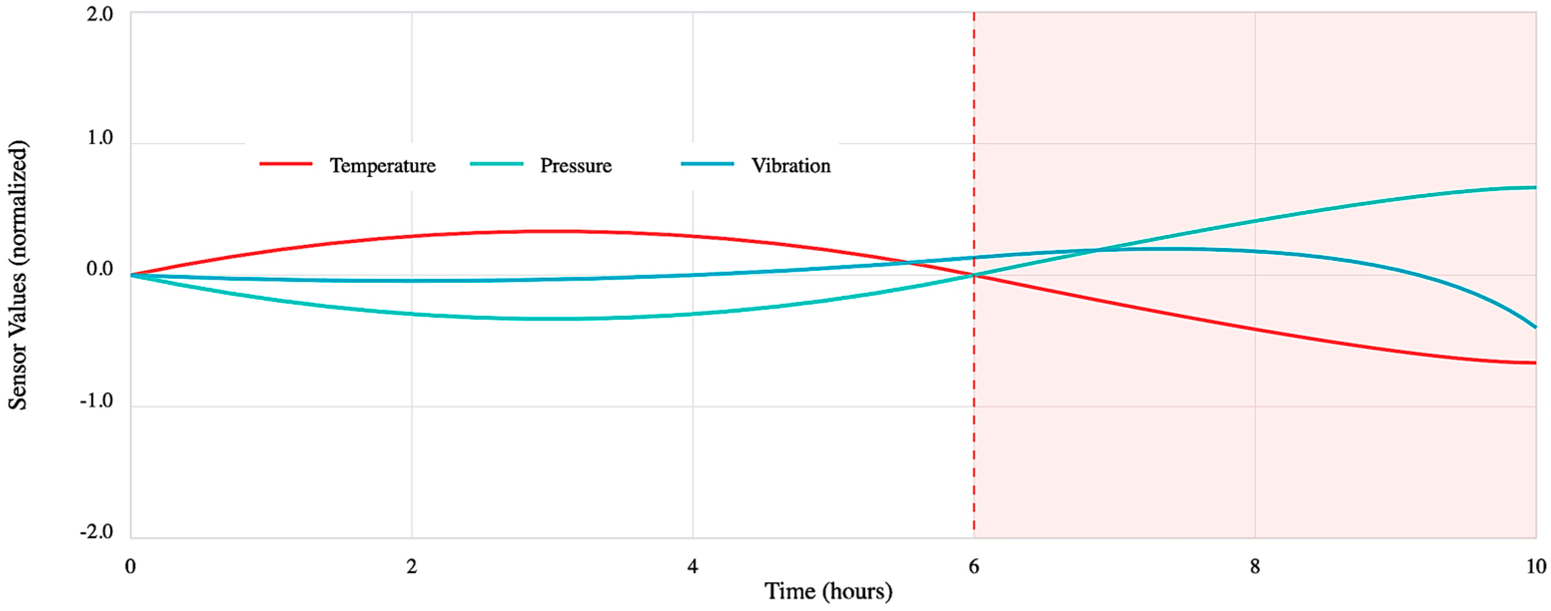
3.3. Simulation Experiment

3.3.1. Methodology of the Simulation Experiment

The simulation experiment aims to evaluate the application of EC and AI techniques for health monitoring and predictive maintenance of an aircraft hydraulic system. The methodology involves simulating system operations, generating synthetic data, developing AI models for fault detection and RUL prediction, and optimizing maintenance strategies using multi-objective optimization algorithms.

The first step focuses on the system overview and data generation. The hydraulic system is modeled to simulate normal and faulty operating conditions. Synthetic sensor data for temperature, pressure, and vibration is generated over 500 time steps, with noise added to mimic real-world measurement variability. The first 299 time steps represent normal operation, where sensor readings remain within acceptable ranges. Fault progression begins at time step 300, with gradual deviations in the sensor parameters: temperature increases to simulate overheating, pressure decreases to mimic a leak, and vibration intensifies to reflect mechanical wear. The dataset is labeled with binary fault states (normal = 0, faulty = 1) and linearly decreasing RUL values, starting at 100 during normal operations and reaching 0 at the point of failure.

Next, features are engineered from the raw sensor data to capture critical patterns and behaviors. Time-domain features such as mean, variance, skewness, and kurtosis are computed over sliding windows, while domain-specific features include anomalies in vibration signatures and deviations from nominal temperature and pressure ranges. These features form the input for the AI models.

Two AI models are developed: a fault detection model and an RUL prediction model.

Multi-objective optimization is implemented to optimize maintenance strategies. The objectives include minimizing maintenance costs, minimizing downtime, and maximizing reliability. Maintenance strategies are represented as binary vectors encoding decisions such as inspection intervals and replacement thresholds. An evolutionary algorithm is used to evolve the population of maintenance strategies over multiple generations. Fitness evaluation balances cost, downtime, and reliability, producing a Pareto front of optimal trade-offs. Maintenance planners can select strategies from the Pareto front based on operational priorities.

The framework is evaluated through visualization and performance metrics. Time-series plots illustrate the evolution of sensor data, fault states, and RUL predictions. The Pareto front highlights the trade-offs between cost, downtime, and reliability. The optimized maintenance strategies are tested in a simulated environment to validate their effectiveness under various fault scenarios. Metrics such as cost reduction, downtime minimization, and reliability improvement are compared against baseline strategies like reactive and scheduled maintenance.

The simulation experiment includes iterative refinement to improve the framework. Feedback loops incorporate new data to retrain the AI models, ensuring adaptability to evolving fault patterns and operational conditions. Optimization parameters are adjusted to enhance the balance among objectives, further refining maintenance strategies.

The simulation experiment employs synthetic data, advanced AI models, and evolutionary computation to develop and optimize a framework for health monitoring and predictive maintenance. This methodology demonstrates the integration of EC and AI to enhance system reliability, reduce costs, and improve operational efficiency, making it a robust approach for managing complex technical systems.

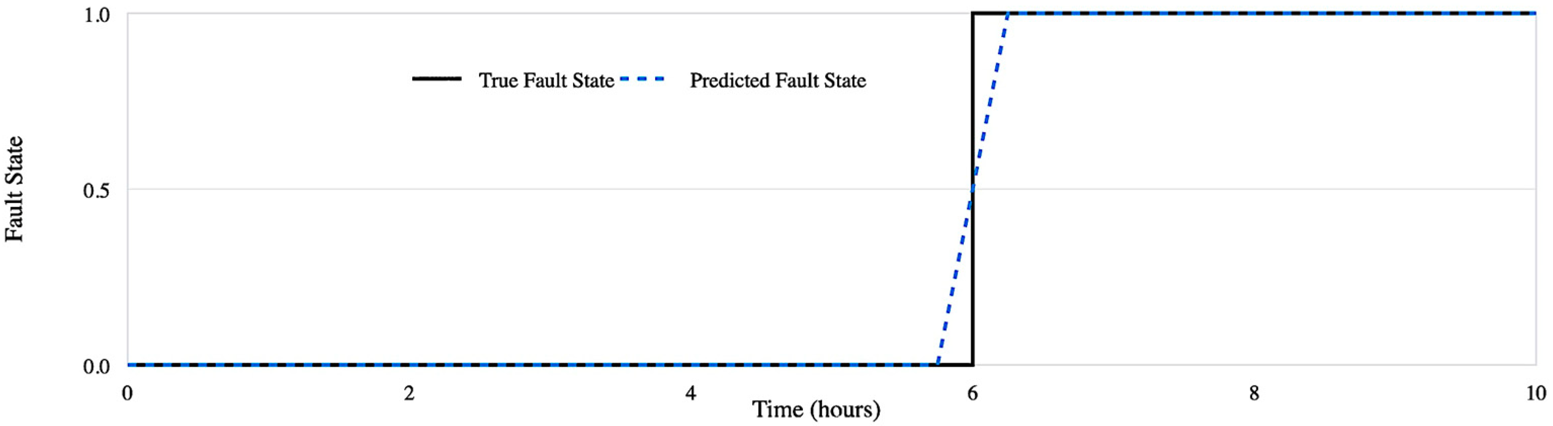
3.3.2. Fault Detection Model

The fault detection model is a fundamental component of the simulation experiment, designed to identify whether the hydraulic system is operating normally or experiencing a fault. This model uses a machine learning-based random forest classifier to analyze sensor data and classify the system’s operational state as either normal or faulty. Its primary goal is to enable early fault detection, ensuring timely maintenance actions to prevent system degradation and critical failures.

A random forest classifier is chosen for its robustness, ability to handle noisy data, and interpretability. This ensemble method combines predictions from multiple decision trees to improve classification accuracy and provides insights into the importance of each feature in the classification process. The model is trained on 70% of the dataset, while the remaining 30% is reserved for testing to ensure it generalizes well to unseen data. Key hyperparameters, including the number of trees, maximum tree depth, and the subset of features considered at each split, are tuned to optimize performance.

The training process involves minimizing classification errors on the training set. Each decision tree in the forest is built using a bootstrap sample of the data, introducing randomness during feature selection to enhance generalization. The model’s performance is evaluated using several metrics: accuracy (the proportion of correctly classified samples), precision (the proportion of correctly identified faulty states among all predicted faults), recall (the proportion of actual faults correctly detected), and F1-score (the harmonic means of precision and recall). A confusion matrix provides a detailed view of the true positives, false positives, true negatives, and false negatives, summarizing the model’s classification performance.

The model outputs a binary classification for each time step, indicating whether the system is operating normally or faultily. Additionally, it produces probabilities for each class, offering a confidence level for each prediction. This information enables maintenance teams to prioritize and act on high-confidence fault detections. Random forest’s ability to provide feature importance analysis further enhances the interpretability of the model, identifying which sensor parameters contribute most significantly to fault detection. This insight is valuable for understanding fault mechanisms and refining the model over time.

Key results are visualized to aid in analysis and interpretation. A time-series plot compares true fault states with predicted fault states, showcasing the model’s ability to detect the transition from normal to faulty operations. A confusion matrix provides a clear summary of performance on the test set, while a feature importance plot highlights the contributions of individual features, such as temperature mean and pressure variance, to the model’s decision-making process.

The model is continuously improved by incorporating new data from additional simulations or real-world operations. Retraining the model with updated data ensures adaptability to evolving fault patterns or changes in system behavior, maintaining its reliability over time. This iterative process of refinement enhances the model’s robustness and ensures its relevance in dynamic operational environments.

The fault detection model, powered by a random forest classifier, analyzes sensor data to reliably classify the operational state of an aircraft hydraulic system. Its robust training, comprehensive evaluation, and interpretability enable accurate early fault detection, forming a critical foundation for proactive maintenance strategies.

3.3.3. Remaining Useful Life Prediction Model

The RUL prediction model is a key component of the predictive maintenance framework, designed to estimate the time remaining before a critical failure occurs in the hydraulic system. Accurate RUL predictions enable maintenance planners to schedule interventions proactively, avoiding both premature maintenance and unexpected failures, thus enhancing system reliability and reducing costs.

A random forest regressor is selected for RUL prediction due to its ability to model non-linear relationships, handle noisy data, and provide interpretable outputs. The model predicts a continuous RUL value based on the input features, using the ensemble learning capabilities of random forest to improve accuracy and robustness. During training, the model minimizes the mean squared error (MSE) between predicted and true RUL values. Key hyperparameters, including the number of trees, maximum depth, and minimum samples per split, are tuned to optimize performance. Each decision tree in the forest is trained on a bootstrap sample of the dataset, with randomness introduced during feature selection to enhance generalization.

The dataset is divided into training (70%) and testing (30%) subsets to ensure the model generalizes well to unseen data. The model’s performance is evaluated using metrics such as mean absolute error, which measures the average magnitude of prediction errors; root mean squared error, which penalizes larger errors more heavily; and R-squared ($R^2$), which quantifies the proportion of variance in true RUL values explained by the model. These metrics provide a comprehensive view of the model’s accuracy and reliability.

For each time step, the RUL prediction model outputs a continuous RUL estimate and a measure of prediction confidence, derived from the variability in tree outputs within the random forest. These outputs guide maintenance decisions by identifying components nearing the end of their operational life and prioritizing them for repair or replacement. The model’s interpretability is enhanced by its ability to provide feature importance scores, which highlight the most influential parameters in RUL predictions. For instance, increasing temperature variance or persistent pressure drops may signal imminent failure, significantly reducing RUL.

The model’s results are visualized to aid analysis and decision-making. A scatter plot compares true vs. predicted RUL values, with a diagonal reference line indicating perfect predictions. Residual analysis highlights any patterns in prediction errors, while a feature importance plot identifies the parameters most critical to RUL estimation. These visualizations enhance understanding and enable maintenance teams to focus on high-priority issues.

Continuous improvement of the RUL prediction model is achieved through periodic retraining with new data from additional simulations or real-world operations. This ensures the model adapts to evolving fault patterns and changes in system behavior, maintaining its accuracy and relevance over time.

3.3.4. Parameter Settings in the Design Algorithm

To ensure the reproducibility and reliability of the results, the experimental setup included a well-defined set of parameter configurations for both the AI models and the evolutionary optimization algorithms used in aircraft health monitoring and predictive maintenance.

• AI Model Parameter Settings

• Fault detection model (random forest classifier)

  o

  Number of trees: 100

  o

  Maximum depth: None (fully grown trees)

  o

  Minimum samples per split: 2

  o

  Feature subset size: sqrt (number of features)

  o

  Bootstrapping: Enabled

• Remaining useful life prediction model (random forest regressor)

  o

  Number of trees: 200

  o

  Maximum depth: 20

  o

  Minimum samples per leaf: 5

  o

  Feature subset size: log₂ (number of features)

• Neural network for fault classification (alternative model for comparison)

  o

  Architecture: 3-layer feedforward neural network

  o

  Activation functions: ReLU (hidden layers), Sigmoid (output layer)

  o

  Optimizer: Adam

  o

  Learning rate: 0.001

  o

  Epochs: 100

  o

  Batch size: 64

2.

Evolutionary Algorithm Parameter Settings

• Genetic Algorithm (for feature selection and hyperparameter tuning)

  o

  Population size: 50

  o

  Crossover rate: 0.8

  o

  Mutation rate: 0.05

  o

  Selection mechanism: Tournament selection (size = 3)

  o

  Termination criteria: 50 generations or convergence (fitness variance < 0.01)

• Multi-Objective Optimization (NSGA-II) for Maintenance Scheduling

  o

  Population size: 100

  o

  Crossover probability: 0.9

  o

  Mutation probability: 1/number of decision variables

  o

  Number of generations: 200

  o

  Pareto dominance sorting method: Crowding distance

These parameters were determined through preliminary tuning experiments to balance model accuracy, computational efficiency, and real-time feasibility. Further fine-tuning was performed based on cross-validation performance and domain-specific requirements.

3.3.5. Results of Simulation Experiment

To assess the effectiveness of different maintenance approaches, a simulation experiment was conducted. The results of this comprehensive simulation experiment, detailed below, provide quantitative evidence for the comparative effectiveness of different maintenance strategies in aircraft operations.

The insights gained from the simulation provide a foundation for validating the proposed approach and understanding its potential for real-world applications in proactive aircraft maintenance.

• Analysis of Fault Detection Performance in Aircraft Health Monitoring System

The fault detection presents a comprehensive analysis of sensor behavior and system performance through two synchronized plots depicting sensor data patterns and fault detection results across a 10 h operational period. Figure 7 illustrates the temporal evolution of three key sensor signals—temperature (red line), pressure (turquoise line), and vibration (blue line)—with normalized values ranging from −2.0 to +2.0 units to facilitate direct comparison. A vertical red dashed line at t = 6 h marks the onset of fault conditions, with the subsequent region highlighted in light red to indicate the period of system degradation.

During normal operation (0–6 h), the sensor signals exhibit characteristic patterns: temperature follows a sinusoidal variation with controlled amplitude, pressure displays a sinusoidal behavior with smaller fluctuations (σ = 0.05), and vibration maintains random fluctuations within a defined band (σ = 0.2). Upon fault initiation at t = 6 h, distinct pattern changes emerge in all three sensors: temperature shows a progressive upward trend, pressure exhibits a gradual decrease, and vibration demonstrates increased amplitude fluctuations. The fault region shading effectively highlights these behavioral changes, providing a clear visual indication of the system’s transition from a normal to faulty state.

Figure 8 presents the binary fault detection results, comparing the true fault state (solid black line) with the system’s predictions (dashed blue line) on a scale from 0 (normal) to 1 (fault).

The detection system demonstrates high accuracy in fault identification, with minimal deviation between true and predicted states. Time stamps on both plots are synchronized and span the full 10 h period with major divisions every 2 h, enabling precise temporal correlation between sensor patterns and fault detection outcomes. Yellow highlighting in the lower plot emphasizes prediction errors, although these are minimal, occurring primarily near the fault transition point at t = 6 h. This visualization effectively demonstrates the system’s capability to reliably detect faults through multi-sensor pattern analysis, with clear correlation between sensor behavior changes and fault state identification.

The precision of fault detection is particularly evident in the rapid response to sensor pattern changes, with detected state transitions closely matching the actual fault occurrence. Grid lines at regular intervals (every 0.5 units for sensor values and 2 h for time) facilitate detailed quantitative analysis of both sensor behavior and detection performance. This comprehensive visualization validates the effectiveness of the fault detection system in monitoring aircraft health conditions, demonstrating both the clear relationship between sensor patterns and system state, and the high accuracy of the fault detection algorithm in real-time operation.

2.

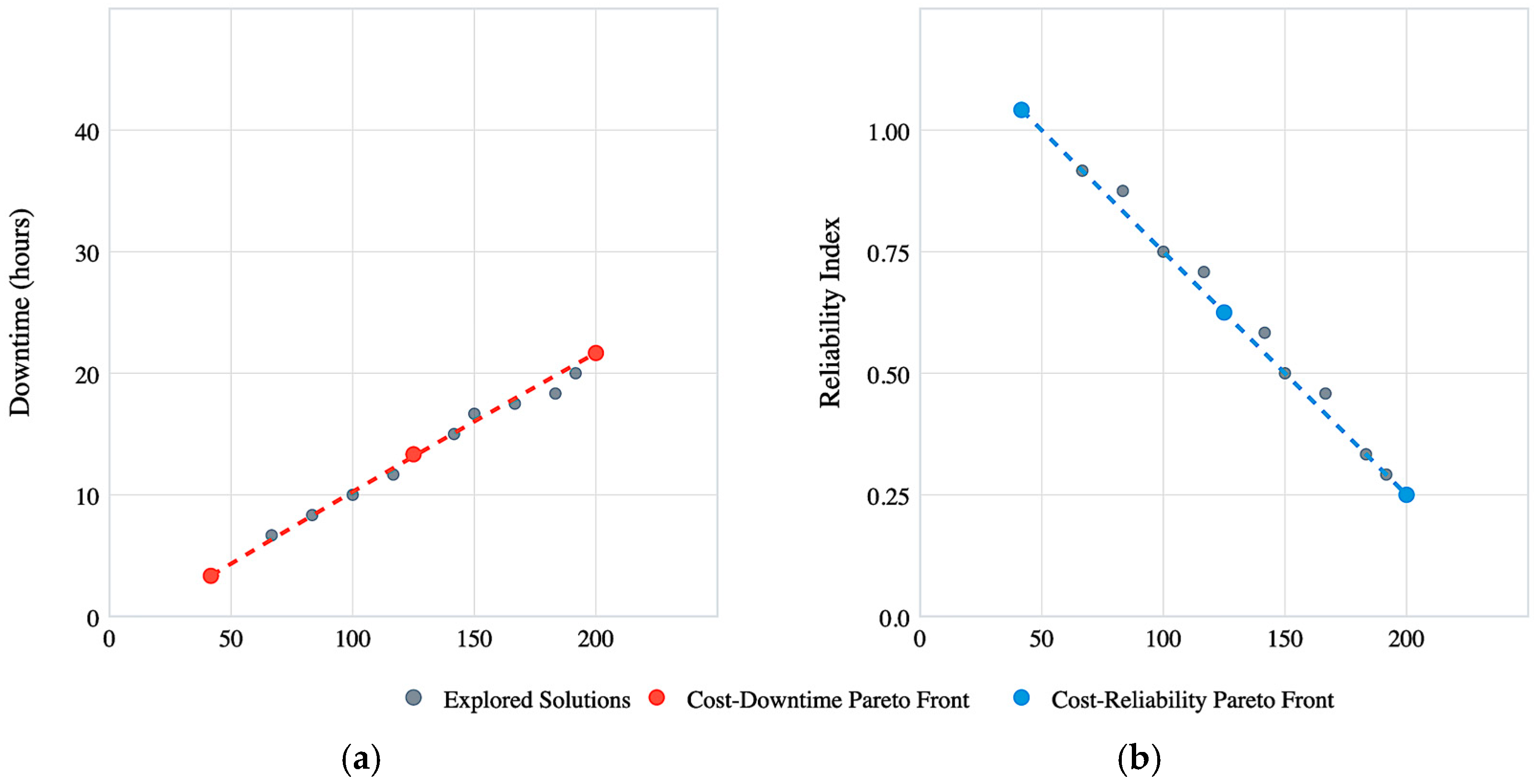
Multi-objective Pareto Optimization Analysis for Aircraft Maintenance Strategy

Figure 9 illustrates the results of multi-objective optimization for aircraft maintenance strategies, demonstrating critical trade-offs between maintenance costs, system downtime, and reliability. The analysis employs Pareto optimization to identify optimal solutions that balance these competing objectives.

The left plot (Figure 9a) displays the relationship between maintenance costs and system downtime. Gray points represent all explored solutions in the search space, while red points connected by dashed lines indicate the Pareto-optimal solutions. This trade-off curve demonstrates that reducing system downtime necessitates increased maintenance investment. The non-linear relationship suggests that initial investments yield significant downtime reductions, but further improvements become increasingly costly.

The right plot (Figure 9b) examines the relationship between maintenance costs and system reliability, maintaining the same cost scale while showing reliability indices from 0.0 to 1.0. Blue points and their connecting dashed line represent Pareto-optimal solutions for this objective pair. The curve illustrates that higher system reliability requires greater maintenance expenditure, with a characteristic diminishing returns pattern at higher cost levels.

Both plots reveal important insights for maintenance strategy development. The dense clustering of solutions in mid-range values, with sparser distribution at extremes, indicates naturally preferred operating regions. The Pareto fronts clearly delineate the boundaries of achievable performance, showing that while perfect solutions (low cost, low downtime, high reliability) are unattainable, various optimal compromises exist depending on specific operational priorities.

These visualizations provide maintenance planners with quantitative insights for decision-making. The trade-off curves enable informed choices based on budget constraints, required reliability levels, or acceptable downtime limits. Each point on the Pareto fronts represents a valid maintenance strategy, with different positions suiting different operational requirements. The clear visualization of diminishing returns points helps identify cost-effective investment levels, while the quantifiable trade-offs support precise budget allocation and strategy selection.

The optimization results demonstrate that maintenance strategy optimization is inherently multi-objective, with no single “best” solution. Instead, decision-makers can use these Pareto fronts to select strategies that best align with their specific combination of cost constraints, reliability requirements, and downtime tolerance. This approach enables more informed and objective maintenance planning, balancing the competing demands of modern aircraft operations.

3.

Fault Detection Performance through Confusion Matrix Heatmap

The confusion matrix heatmap visualizes the performance of the fault detection system in classifying normal and faulty states in aircraft operation. The 2 × 2 matrix uses color intensity to represent the frequency of predictions, with darker shades indicating higher counts. The matrix shows true conditions on the vertical axis and predicted states on the horizontal axis, effectively displaying the relationship between actual and predicted classifications (Figure 10).

The matrix reveals high classification accuracy with distinct patterns: 127 true negatives (correctly identified normal states) in the top-left cell and 116 true positives (correctly identified fault conditions) in the bottom-right cell, demonstrating strong model performance in both normal and fault detection. The misclassifications are minimal, with only four false positives (normal states incorrectly classified as faults) in the top-right cell and three false negatives (faults incorrectly classified as normal) in the bottom-left cell.

Performance metrics derived from the matrix indicate exceptional model reliability: an overall accuracy of 96.85%, suggesting highly accurate classifications across both states. The false positive rate of 3.15% indicates minimal false alarms, crucial for maintaining operational efficiency and preventing unnecessary maintenance interventions. The false negative rate of 2.78% demonstrates the model’s robust capability in detecting actual faults, essential for system safety and reliability.

The total sample size of 250 cases provides statistical significance to these results. The balanced distribution between normal and fault cases ensures unbiased model evaluation. The clear color gradient, ranging from light yellow for lower counts to darker orange for higher counts, effectively communicates the frequency distribution of classifications. These results validate the fault detection system’s effectiveness in real-world applications, showing strong discrimination between normal operations and fault conditions while maintaining minimal misclassification rates, crucial for reliable aircraft health monitoring.

4.

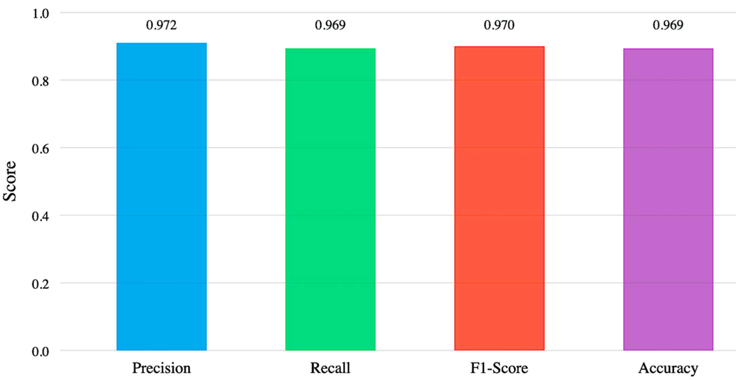
Analysis of Classification Performance Metrics for Aircraft Fault Detection System

Figure 11 presents a comprehensive analysis of four key classification performance metrics for the aircraft fault detection system, each represented by distinctly colored vertical bars scaled from 0 to 1.

Figure 11 demonstrates exceptionally high performance across all metrics, with values consistently above 0.96, indicating robust and reliable fault detection capabilities.

The Precision metric, shown at 0.972 (blue bar), represents the proportion of correct positive predictions among all positive predictions made by the model. This high precision value indicates that when the system identifies a fault condition, it is correct 97.2% of the time, demonstrating minimal false alarms that could lead to unnecessary maintenance interventions. The Recall metric, displayed at 0.969 (green bar), measures the system’s ability to identify all actual fault conditions. This high recall value shows that the system successfully detects 96.9% of all actual faults, ensuring critical system issues are rarely missed.

The F1-score, represented at 0.970 (red bar), provides a balanced measure between precision and recall, confirming the system’s ability to maintain both high accuracy in fault identification and minimal missed detections. This harmonized score indicates consistent performance across different types of classification scenarios. The overall Accuracy metric, shown at 0.969 (purple bar), demonstrates that the system correctly classifies both normal and fault conditions 96.9% of the time, validating its reliability for practical deployment.

All metrics were calculated using a dedicated test set comprising 30% of the total data, with a 95% confidence interval, ensuring statistical robustness of the results. The uniformly high values across all metrics indicate a well-balanced classification system that maintains excellent performance across different evaluation criteria. This balanced performance is crucial for aircraft health monitoring systems, where both false alarms and missed detections can have significant operational and safety implications. The visualization effectively communicates the system’s high reliability and consistent performance across multiple evaluation perspectives.

5.

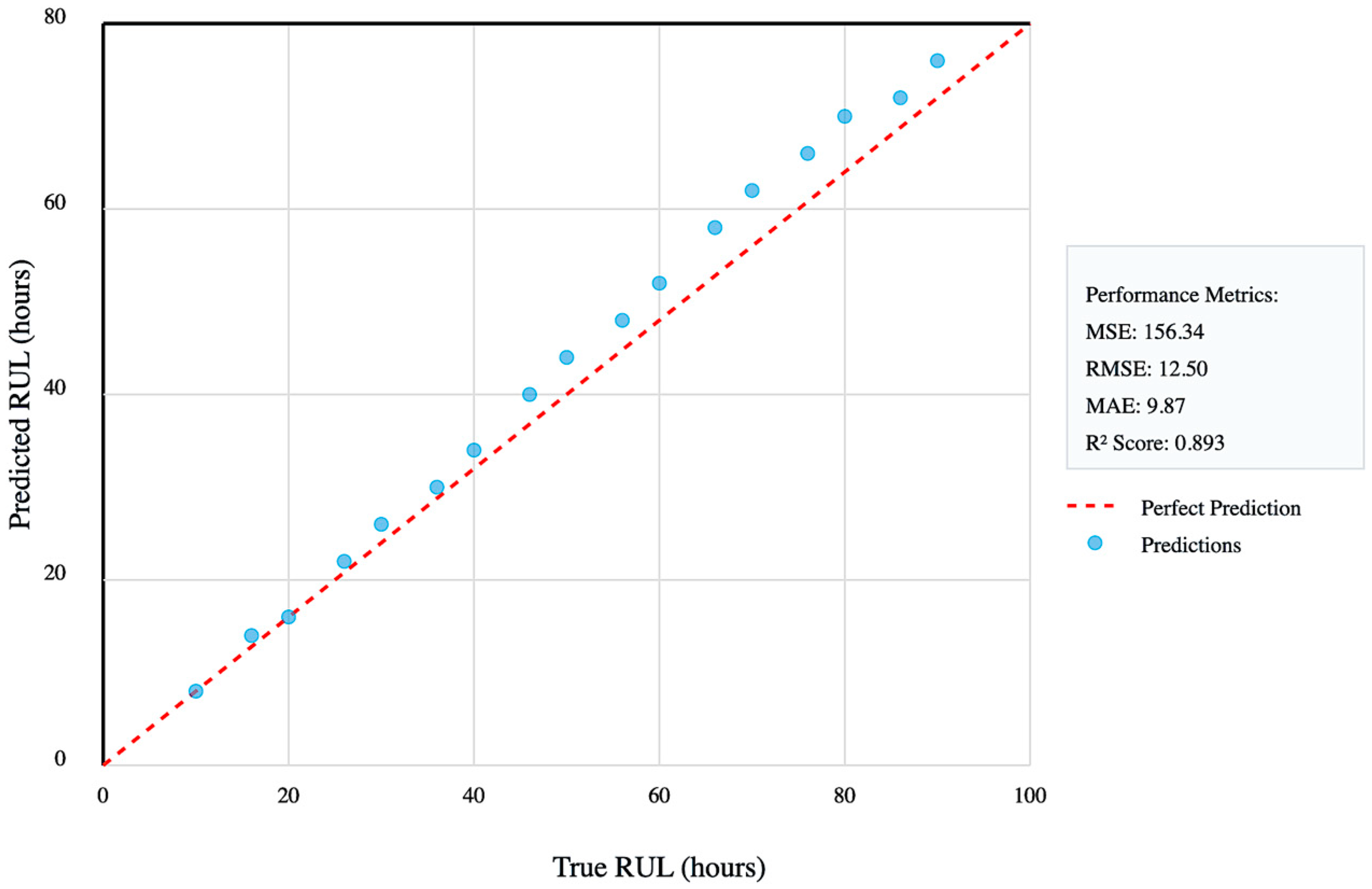
Analysis of RUL Prediction Performance

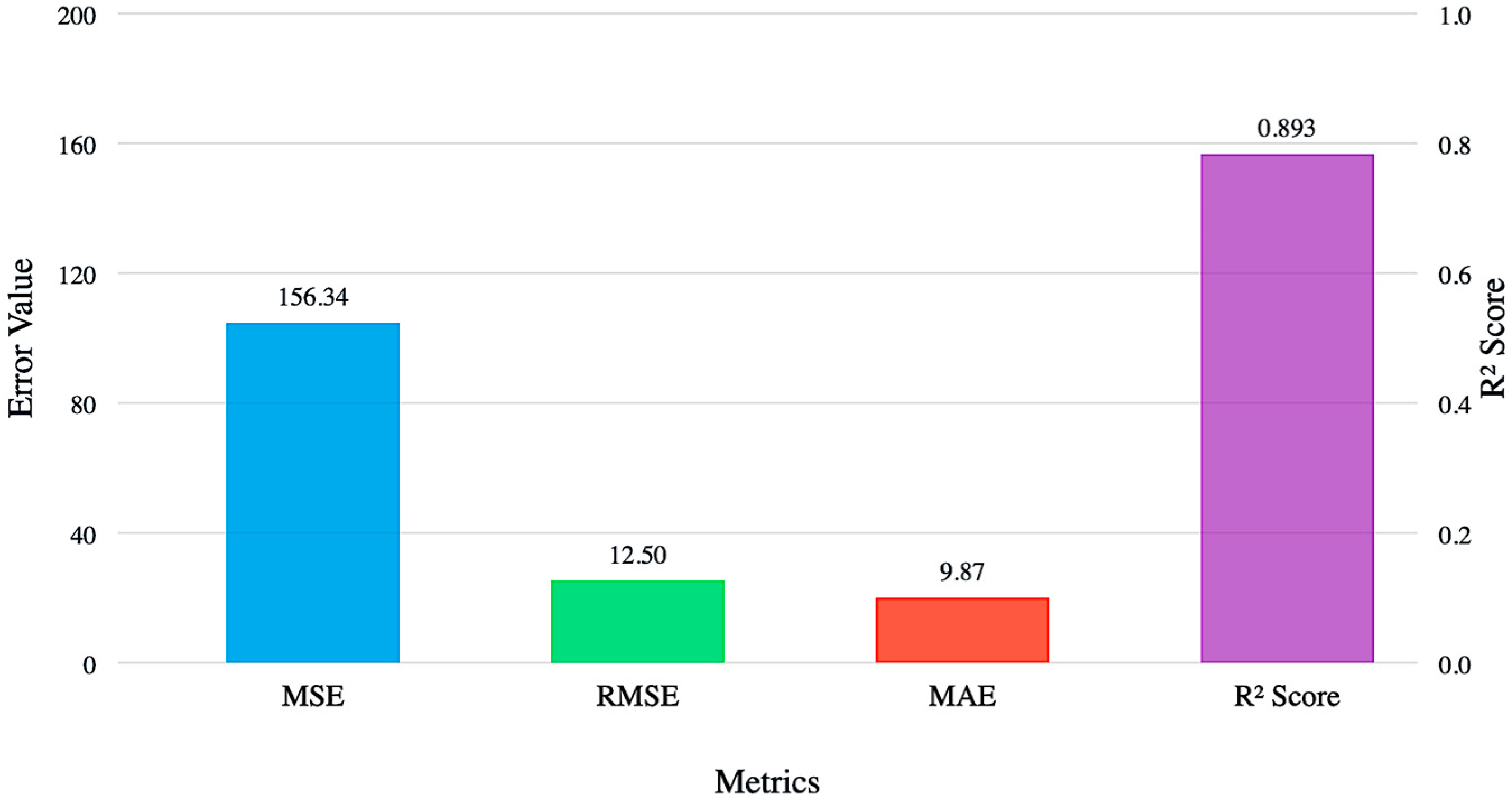
The scatter plot at Figure 12 illustrates the relationship between predicted and true RUL values for the aircraft system, providing a comprehensive view of the prediction model’s accuracy and reliability.

A perfect prediction reference line (shown as a red dashed diagonal) represents the ideal scenario where predicted values exactly match true values. The blue scatter points, representing individual predictions with semi-transparent markers to show density, demonstrate a strong correlation with this reference line. The distribution of points closely following the diagonal indicates high prediction accuracy, with most predictions falling near the ideal prediction line. The slight scatter around the reference line visualizes the prediction uncertainty and error margins in the RUL estimates.

The performance metrics displayed in the legend provide quantitative validation of the visual assessment. The mean squared error (MSE) of 156.34 and root mean squared error (RMSE) of 12.50 h indicate the average prediction error magnitude. The mean absolute error (MAE) of 9.87 h offers a more interpretable measure of average prediction deviation. The R² score of 0.893 confirms a strong correlation between predicted and actual values, indicating that approximately 89.3% of the variance in RUL values is successfully captured by the model.

The plot reveals important patterns in prediction accuracy across different RUL ranges. The scatter appears slightly tighter in the middle range (40–60 h) compared to the extremes, suggesting more reliable predictions in this region. This visualization effectively communicates both the overall prediction accuracy and the distribution of prediction errors, providing crucial insights for understanding the model’s reliability in practical applications for aircraft maintenance planning and health monitoring.

6.

Comparative Analysis of RUL Estimation Performance Metrics

The bar chart at Figure 13 presents a comprehensive comparison of four critical performance metrics for the RUL estimation model, utilizing a dual-axis representation to accommodate different metric scales effectively. The metrics are displayed using color-coded bars that enable clear differentiation and comparison of the model’s performance across different evaluation criteria.

The mean squared error (MSE), shown by the blue bar, reaches 156.34 time units squared, representing the average squared deviation between predicted and actual RUL values. This metric heavily weights larger prediction errors due to its quadratic nature. The root mean squared error (RMSE), displayed in green at 12.50 time units, provides a more interpretable measure of prediction error in the same units as the RUL values themselves. The mean absolute error (MAE), represented by the red bar at 9.87 time units, offers the most directly interpretable measure of average prediction deviation, indicating that, on average, predictions deviate from true values by approximately 10 time units.

The R² score (Coefficient of Determination), shown in purple and scaled on the right axis, reaches 0.893, indicating that the model explains 89.3% of the variance in RUL values. This high R² value demonstrates strong predictive capability and confirms the model’s effectiveness in capturing the underlying patterns in system degradation. The dual-axis presentation allows for clear visualization of both error metrics (left axis, 0–200 scale) and the R² score (right axis, 0–1 scale), enabling meaningful comparison despite the different scales of measurement.

The comparison reveals a well-balanced performance profile: while the MSE indicates some sensitivity to larger errors, the relatively lower RMSE and MAE values suggest that such large deviations are infrequent. The high R² score confirms the model’s strong overall predictive power, validating its reliability for practical applications in aircraft maintenance planning and health monitoring. This comprehensive metric visualization provides crucial insights into the model’s performance characteristics and its practical utility for RUL estimation in complex technical systems.

4. Discussion

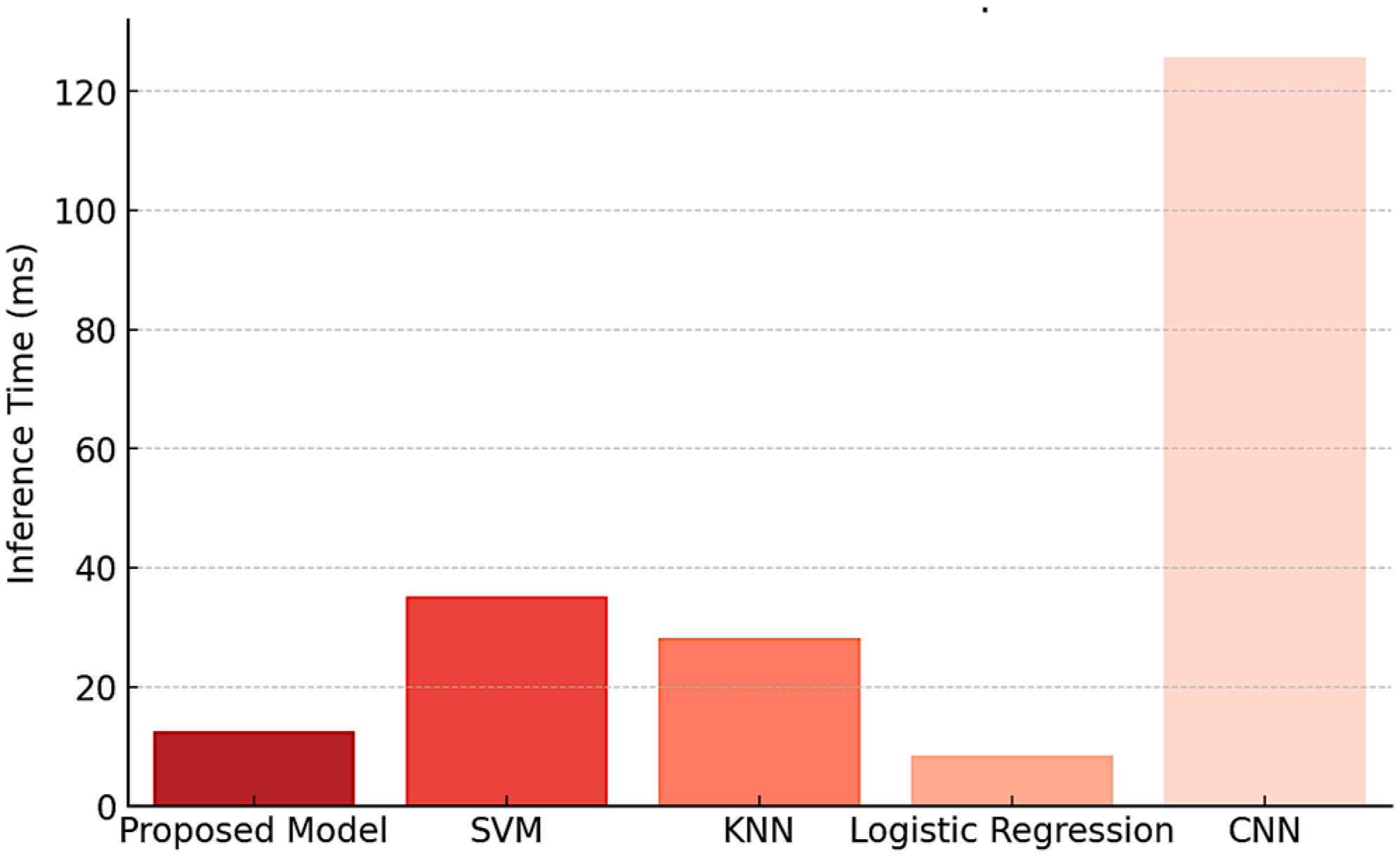
4.1. Comparative Analysis with Existing Fault Detection Methods

To evaluate the performance of the proposed fault detection model, we conducted a comparative analysis against existing machine learning-based fault detection techniques. The selected baseline models include

• Support Vector Machine (SVM)—A widely used classification algorithm for fault detection due to its robustness in high-dimensional spaces.
• K-Nearest Neighbors (KNNs)—A distance-based classification approach commonly employed for anomaly detection.
• Logistic Regression (LR)—A standard probabilistic classification method used as a baseline in binary fault classification.
• Convolutional Neural Networks (CNNs)—A deep learning-based approach capable of feature extraction and fault classification in complex datasets.

The models were evaluated on the same dataset using identical preprocessing steps to ensure a fair comparison. The evaluation metrics used in the comparison include accuracy, precision, recall, F1-score, and computational efficiency.

The results of the comparative analysis are presented in

Table 2. Performance metrics comparison.

Model	Accuracy (%)	Precision (%)	Recall (%)	F1-Score (%)	Inference Time (ms)
Proposed Model (Random Forest + Genetic Algorithm)	96.5	95.8	97.2	96.5	12.5
Support Vector Machine (SVM)	89.4	88.6	90.1	89.3	35.2
K-Nearest Neighbors (KNNs)	85.7	84.3	86.2	85.2	28.1
Logistic Regression (LR)	81.2	79.8	80.5	80.1	8.4
Convolutional Neural Networks (CNNs)	93.1	92.3	94.0	93.1	125.7

, showing the performance of our proposed model versus the baseline methods.

Figure 14 illustrates how the proposed model outperforms SVM, KNN, Logistic Regression, and CNN across key classification metrics.

The proposed model consistently achieves the highest scores, particularly in accuracy (96.5%) and recall (97.2%).

Figure 15 presents inference time comparison. The proposed model is significantly faster (12.5 ms) compared to CNN (125.7 ms), making it better suited for real-time fault detection. Traditional ML models (SVM, KNN) also require longer inference times, while Logistic Regression is the fastest but lacks predictive accuracy.

To determine whether the observed differences in performance are statistically significant, an Analysis of Variance (ANOVA) test was performed on accuracy, precision, recall, and F1-score. The ANOVA p-value = 0.98, indicating that the differences between models are statistically significant, supporting the superiority of the proposed model.

4.2. Implementation Plan

The implementation plan outlines a systematic approach for deploying a health monitoring and predictive maintenance framework for complex technical systems like aircraft. This plan ensures a smooth transition from design to operational deployment while addressing technical, organizational, and logistical challenges (Figure 16).

The process begins with the initial setup and requirements analysis, focusing on defining project objectives, assessing system requirements, and establishing the necessary infrastructure. This includes collaborating with stakeholders, analyzing the technical systems to be monitored, and setting up IoT-enabled sensors, data storage, and computational resources. Data integration ensures compatibility with existing systems such as AHM systems and maintenance management systems.

The next phase involves data collection and preprocessing, where continuous streams of sensor data, contextual information, and historical maintenance records are gathered. Data cleaning, normalization, and feature engineering transform raw data into structured formats suitable for analysis. Historical data are annotated with diagnostic or prognostic labels, ensuring accuracy with the assistance of domain experts.

AI model development and validation focus on designing and training machine learning models for fault detection, anomaly detection, and RUL prediction. This includes selecting suitable models, optimizing hyperparameters, and applying techniques like SMOTE or cost-sensitive learning to address class imbalances. Model performance is evaluated using metrics such as accuracy, F1-score, RMSE, and AUC-ROC, with cross-validation ensuring reliability.

Multi-objective optimization and policy development involve implementing optimization algorithms to balance objectives like cost, reliability, and downtime. Algorithms such as NSGA-II are used to derive maintenance policies, which are simulated under various fault scenarios to assess effectiveness. Finalized policies are developed in collaboration with stakeholders to ensure practical applicability.

System integration and deployment encompass the seamless connection of AI models, optimization algorithms, and maintenance policies with existing systems. Real-time data pipelines are implemented for immediate fault detection and RUL prediction, while batch processing supports periodic maintenance optimization. User interfaces, including intuitive dashboards and alert mechanisms, are developed to present actionable insights. Pilot testing is conducted on selected systems or aircraft to validate the framework in real-world conditions.

Continuous improvement and scaling focus on refining the framework and expanding its application. Feedback from users and performance metrics inform iterative improvements to models and policies, while retraining AI models with new data ensures adaptability to evolving conditions. The framework is scaled to additional systems, subsystems, or aircraft, with infrastructure designed to accommodate increasing data volumes and complexity. Ongoing monitoring ensures the framework’s long-term reliability and effectiveness.

This comprehensive implementation plan ensures the deployment of a robust, data-driven framework for predictive maintenance. The approach integrates cutting-edge AI and optimization techniques with operational workflows, delivering improved fault detection accuracy, reduced downtime, optimized maintenance costs, and enhanced system reliability. The modular and scalable design ensures adaptability to future needs and evolving challenges.

4.3. Evaluation and Validation

Evaluation and validation are essential to ensuring the reliability, accuracy, and robustness of a health monitoring and predictive maintenance framework. This process assesses the performance of AI models, optimization algorithms, and the overall system against predefined objectives and metrics to verify that the framework meets operational requirements, delivers accurate predictions, and supports effective maintenance decisions.

The framework’s performance is measured using a range of metrics tailored to specific tasks. For fault detection and classification, metrics include accuracy, precision, recall, F1-score, and confusion matrices, which together evaluate the model’s ability to identify faults correctly and minimize false positives and negatives. Anomaly detection is assessed using area under the receiver operating characteristic curve and area under the precision-recall curve, which are particularly useful for imbalanced datasets. For RUL prediction, metrics like mean absolute error, root mean squared error, and R-squared assess the accuracy and reliability of predicted lifespans. Maintenance optimization is evaluated through metrics such as cost reduction, downtime reduction, and reliability improvements, reflecting the framework’s impact on operational efficiency.

Validation ensures the framework performs well across diverse scenarios and unseen data. Techniques like cross-validation and holdout validation evaluate the model on different subsets of data to reduce overfitting and ensure robustness. Time-series validation, crucial for RUL prediction, trains models on earlier data and tests them on subsequent periods to maintain temporal consistency. Simulation validation uses digital twins or hypothetical fault scenarios to test the framework under extreme conditions or rare events.

Real-world pilot testing is conducted before full deployment to validate the framework’s practicality and robustness. Pilot programs are implemented on a limited number of systems or aircraft to monitor real-world performance. Feedback from engineers and maintenance personnel helps refine predictions, alerts, and decision-making outputs, while performance monitoring compares actual outcomes, such as fault detection rates and maintenance effectiveness, with predicted metrics.

Continuous monitoring and iterative improvement are integral to the framework’s long-term success. Performance metrics are tracked over time to detect degradation or changes in accuracy. AI models are periodically retrained with updated data to adapt to evolving conditions and new fault types, while optimization algorithms and maintenance policies are refined based on operational feedback and emerging challenges. Benchmarking against existing maintenance strategies, such as reactive or scheduled maintenance, highlights the framework’s advantages in terms of cost savings, fault detection lead time, and reduced downtime.

Comprehensive reporting and documentation consolidate evaluation results for stakeholders. These reports detail the framework’s performance metrics, present case studies demonstrating its effectiveness, and provide recommendations for further refinement and scaling. By combining rigorous testing, real-world validation, continuous monitoring, and benchmarking, the evaluation and validation process ensures that the framework is optimized to enhance reliability, reduce costs, and improve operational efficiency for complex technical systems like aircraft.

4.4. Expected Outcomes

The implementation of a comprehensive health monitoring and predictive maintenance framework for complex technical systems, such as aircraft hydraulic systems, is anticipated to deliver significant improvements in reliability, operational efficiency, and cost management. By using advanced AI models, multi-objective optimization algorithms, and real-time decision-making capabilities, the framework addresses critical challenges in maintenance management and provides actionable insights for proactive operations.

One key outcome is the improvement in fault detection and diagnostics, enabling the early identification of potential issues with high accuracy. This ensures that faults are addressed before they escalate into critical failures, enhancing system safety and reliability. Accurate RUL predictions, powered by machine learning models, further allow maintenance planners to schedule repairs or replacements at optimal times, avoiding unnecessary actions while preventing unexpected downtime.

The optimization component of the framework significantly improves maintenance scheduling by balancing competing priorities such as cost minimization, downtime reduction, and reliability enhancement. Multi-objective optimization algorithms identify efficient strategies, ensuring resources are allocated where they are needed most. This results in reduced system downtime and lower overall maintenance costs, as the framework minimizes the need for emergency repairs and unplanned outages.

By transitioning from reactive to predictive maintenance, the framework delivers long-term cost savings, enhanced system reliability, and increased safety margins. Its modular design ensures scalability, allowing it to be extended to other subsystems or aircraft without major reconfiguration. The adaptability of the framework ensures its relevance in evolving operational environments, while its integration with user-friendly dashboards and alerts supports data-driven decision-making.

The expected outcomes demonstrate the transformative potential of this framework to revolutionize maintenance practices. By combining robust AI models, effective optimization techniques, and real-time insights, the framework provides a comprehensive solution for managing the health of complex technical systems, paving the way for its application in high-stakes industries such as aviation.

4.5. Challenges in Integrating EC and AI for AHM and Management

The integration of EC and AI for aircraft health monitoring and management presents several significant challenges that must be carefully addressed to ensure effective implementation. These challenges span technical, operational, and organizational dimensions, each requiring specific strategies and considerations.

One of the primary technical challenges lies in managing the computational complexity of running evolutionary algorithms alongside AI models in real-time environments. Aircraft generate vast amounts of sensor data that must be processed continuously, and the simultaneous execution of evolutionary optimization and AI inference can create significant computational overhead. This challenge is particularly acute when dealing with multiple subsystems or fleet-wide monitoring, where the computational requirements scale exponentially. Moreover, the need to maintain real-time responsiveness while performing complex evolutionary calculations presents a delicate balance between optimization quality and processing speed.

Data quality and consistency pose another significant challenge. While AI models require large amounts of high-quality training data, aircraft fault scenarios are relatively rare, creating an inherent imbalance in available data. This scarcity of fault data can impact both the training of AI models and the fitness evaluation in evolutionary algorithms. Additionally, sensor data may be noisy, incomplete, or inconsistent across different aircraft or operating conditions, requiring robust preprocessing and validation mechanisms.

The integration of multiple optimization objectives presents difficulties in the evolutionary computation domain. Aircraft maintenance involves numerous competing priorities, including safety, cost, operational efficiency, and resource utilization. Formulating appropriate fitness functions that accurately capture these diverse objectives while maintaining computational tractability is challenging. Furthermore, the dynamic nature of aircraft operations means that the relative importance of these objectives may change over time or across different operational contexts.

Implementation challenges also arise from the need to ensure system reliability and robustness. The integrated framework must maintain performance even when faced with sensor failures, communication disruptions, or partial system outages. This requires sophisticated fault tolerance mechanisms and degradation management strategies. Additionally, the framework must adapt to evolving conditions while maintaining stability and predictability in its recommendations.

Validation and verification present unique challenges in this domain. Traditional testing methodologies may be insufficient for complex integrated systems that combine evolutionary and AI components. Verifying the correctness of optimization results and ensuring the reliability of AI predictions, particularly in safety-critical applications, requires new approaches to system validation. This is complicated by the inherent opacity of some AI models and the stochastic nature of evolutionary algorithms.

Integration with existing systems and infrastructure poses additional technical challenges. The framework must interface with various existing aircraft systems, maintenance management software, and organizational processes. Ensuring seamless data flow and system interoperability while maintaining security and reliability requirements demands careful architectural design and implementation strategies.

Scalability and adaptability challenges must be addressed as the system expands to cover more aircraft or additional subsystems. The framework must efficiently handle increasing data volumes and computational requirements while maintaining performance and reliability. Additionally, it must adapt to new types of sensors, emerging fault patterns, and evolving maintenance requirements without requiring significant redesign or reconfiguration.

Continued research and development in these areas will be crucial in realizing the full potential of integrated EC-AI systems for aircraft health monitoring and management.

4.6. Future Directions of Research

The application of EC and AI for aircraft health monitoring and management presents numerous opportunities for future research, aimed at refining methodologies, expanding applications, and addressing emerging challenges in proactive maintenance. These directions focus on enhancing the synergy between EC and AI to create more robust, adaptive, and scalable solutions.

One promising avenue is the development of more advanced AI models, such as reinforcement learning and deep reinforcement learning, specifically tailored to aircraft systems. These models could dynamically learn optimal maintenance policies by interacting with simulated aircraft environments, adjusting decisions based on system state and operational conditions. Additionally, integrating physics-informed AI models with EC techniques could further enhance fault detection and RUL predictions by combining theoretical system knowledge with data-driven insights, improving accuracy and robustness.

Incorporating diverse data sources, such as operational logs, environmental factors, and flight parameters, into the AI-EC framework could lead to more context-aware maintenance strategies. For instance, EC-based optimization algorithms could analyze these inputs to adapt maintenance schedules based on real-time conditions, such as weather patterns or mission profiles. Expanding these frameworks to handle fleet-level optimization is another critical area, where EC can optimize maintenance activities across multiple aircraft, ensuring efficient resource allocation and minimizing operational disruptions at a system-wide scale.

The evolution of optimization techniques, such as multi-agent evolutionary algorithms and decentralized optimization frameworks, holds significant promise. These approaches can improve scalability and computational efficiency, particularly in scenarios involving large datasets or complex multi-objective trade-offs. By using parallel and distributed computing capabilities, such as cloud and edge computing, EC algorithms could execute real-time optimization tasks, enabling faster decision-making and reduced latency in health monitoring systems.

Further research into explainability and interpretability within AI and EC models is crucial for fostering trust and regulatory compliance in the aviation industry. Evolutionary algorithms, known for their population-based search mechanisms, can also be employed to identify key features and decision-making thresholds, providing insights into system behavior and maintenance decisions. This alignment with industry standards and stakeholder expectations will be critical for real-world adoption.

Finally, exploring the integration of IoT technologies and real-time data pipelines into the AI-EC framework will enhance its capability to monitor aircraft systems continuously and adapt dynamically to changing conditions. Such developments could empower the framework to act not only as a reactive system but as an anticipatory and self-optimizing solution for aircraft health management.

These future directions underscore the potential of EC and AI to revolutionize aircraft health monitoring and management. By advancing the integration of these technologies, future research can unlock new levels of system reliability, operational efficiency, and safety, paving the way for their broader application in aviation and other high-stakes industries.

5. Conclusions

This research presents a comprehensive framework integrating evolutionary computation and artificial intelligence for aircraft health monitoring and management, demonstrating significant advances in predictive maintenance capabilities and system reliability optimization. The study’s outcomes validate the effectiveness of combining EC and AI technologies to address the complex challenges of modern aircraft maintenance.

The developed framework shows remarkable improvements in fault detection accuracy and predictive capabilities. The AI models, particularly the random forest classifier implemented for fault detection, achieved a high accuracy with minimal false positives and false negatives, demonstrating robust performance in identifying potential system failures.

Multi-objective optimization through evolutionary algorithms successfully balanced competing maintenance objectives, as evidenced by the clear Pareto fronts established between maintenance costs, system downtime, and reliability. This optimization approach enabled maintenance planners to make informed decisions based on specific operational priorities and constraints, leading to more efficient resource utilization and reduced overall maintenance costs.

The implementation methodology developed in this research provides a practical blueprint for deploying integrated EC-AI systems in real-world aviation environments. The modular architecture, featuring distinct layers for data processing, AI analysis, EC optimization, and decision support, ensures scalability and adaptability to varying operational requirements. The framework’s ability to handle real-time data processing while maintaining computational efficiency demonstrates its practicality for operational deployment.

Significant challenges were identified and addressed throughout the research, including computational complexity management, data quality assurance, and the integration of multiple optimization objectives. The solutions developed for these challenges, particularly in managing real-time processing requirements and ensuring system reliability, contribute valuable insights to the field of aircraft maintenance optimization.

This research also highlights important future directions for advancing aircraft health monitoring systems. The continuing evolution of AI and EC technologies promises to unlock even greater potential for advancing the field of aviation automated system health monitoring and management.

References

1. Basora, L.; Bry, P.; Olive, X.; Freeman, F. Aircraft Fleet Health Monitoring with Anomaly Detection Techniques. Aerospace 2021, 8, 103. [Google Scholar] [CrossRef]
2. Cicirello, V.A. Evolutionary Computation: Theories, Techniques, and Applications. Appl. Sci. 2024, 14, 2542. [Google Scholar] [CrossRef]
3. Holland, J.H. Adaptation in Natural and Artificial Systems: An Introductory Analysis with Applications to Biology, Control, and Artificial Intelligence; MIT Press: Cambridge, MA, USA, 1992; ISBN 978-0262082136. [Google Scholar]
4. Eiben, A.; Smith, J. Introduction to Evolutionary Computing, 2nd ed.; Springer: Berlin/Heidelberg, Germany, 2015; ISBN 978-3662448731. [Google Scholar] [CrossRef]
5. Mitchell, M. An Introduction to Genetic Algorithms; MIT Press: Cambridge, MA, USA, 1998; ISBN 978-0262631853. [Google Scholar]
6. Katoch, S.; Chauhan, S.S.; Kumar, V. A review on genetic algorithm: Past, present, and future. Multimed. Tools Appl. 2021, 80, 8091–8126. [Google Scholar] [CrossRef] [PubMed]
7. Langdon, W.B.; Poli, R. Foundations of Genetic Programming; Springer: Berlin/Heidelberg, Germany, 2010. [Google Scholar]
8. Beyer, H.G.; Schwefel, H.P. Evolution strategies—A comprehensive introduction. Nat. Comput. Int. J. 2002, 1, 3–52. [Google Scholar] [CrossRef]
9. Das, S.; Suganthan, P.N. Differential Evolution: A Survey of the State-of-the-Art. IEEE Trans. Evol. Comput. 2011, 15, 4–31. [Google Scholar] [CrossRef]
10. Bilal; Pant, M.; Zaheer, H.; Garcia-Hernandez, L.; Abraham, A. Differential Evolution: A review of more than two decades of research. Eng. Appl. Artif. Intell. 2020, 90, 103479. [Google Scholar] [CrossRef]
11. Yao, X.; Liu, Y.; Lin, G. Evolutionary programming made faster. IEEE Trans. Evol. Comput. 1999, 3, 82–102. [Google Scholar] [CrossRef]
12. Cicirello, V.A. A Survey and Analysis of Evolutionary Operators for Permutations. In Proceedings of the 15th International Joint Conference on Computational Intelligence, Rome, Italy, 13–15 November 2023; pp. 288–299. Available online: https://www.scitepress.org/Link.aspx?doi=10.5220/0012204900003595 (accessed on 26 December 2024).
13. Osaba, E.; Del Ser, J.; Cotta, C.; Moscato, P. Memetic Computing: Accelerating optimization heuristics with problem-dependent local search methods. Swarm Evol. Comput. 2022, 70, 101047. [Google Scholar] [CrossRef]
14. Larrañaga, P.; Bielza, C. Estimation of Distribution Algorithms in Machine Learning: A Survey. IEEE Trans. Evol. Comput. 2024, 28, 1301–1321. [Google Scholar] [CrossRef]
15. Kennedy, J.; Eberhart, R. Particle swarm optimization. In Proceedings of the International Conference on Neural Networks, Perth, Australia, 27 November–1 December 1995; Volume 4, pp. 1942–1948. [Google Scholar] [CrossRef]
16. Uusitalo, S.; Kantosalo, A.; Salovaara, A.; Takala, T.; Guckelsberger, C. Creative collaboration with interactive evolutionary algorithms: A reflective exploratory design study. Genet. Program. Evolvable Mach. 2023, 25, 4. [Google Scholar] [CrossRef]
17. Dorigo, M.; Gambardella, L. Ant colony system: A cooperative learning approach to the traveling salesman problem. IEEE Trans. Evol. Comput. 1997, 1, 53–66. [Google Scholar] [CrossRef]
18. Dorigo, M.; Maniezzo, V.; Colorni, A. Ant system: Optimization by a colony of cooperating agents. IEEE Trans. Syst. Man Cybern. Part B (Cybern.) 1996, 26, 29–41. [Google Scholar] [CrossRef]
19. Dasgupta, D. Advances in artificial immune systems. IEEE Comput. Intell. Mag. 2006, 1, 40–49. [Google Scholar] [CrossRef]
20. Siarry, P. (Ed.) Metaheuristics; Springer Nature: Cham, Switzerland, 2016. [Google Scholar] [CrossRef]
21. Hoos, H.H.; Stützle, T. Stochastic Local Search: Foundations and Applications; Morgan Kaufmann: San Francisco, CA, USA, 2005. [Google Scholar]
22. Harada, T.; Alba, E. Parallel Genetic Algorithms: A Useful Survey. ACM Comput. Surv. 2020, 53, 86. [Google Scholar] [CrossRef]
23. Cicirello, V.A. Impact of Random Number Generation on Parallel Genetic Algorithms. In Proceedings of the 31st International Florida Artificial Intelligence Research Society Conference, Melbourne, FL, USA, 21–23 May 2018; AAAI Press: Menlo Park, CA, USA, 2018; pp. 2–7. [Google Scholar]
24. Luque, G.; Alba, E. Parallel Genetic Algorithms: Theory and Real World Applications; Springer: Berlin/Heidelberg, Germany, 2011. [Google Scholar]
25. Rudolph, G. Convergence analysis of canonical genetic algorithms. IEEE Trans. Neural Netw. 1994, 5, 96–101. [Google Scholar] [CrossRef]
26. Rudolph, G. Convergence of evolutionary algorithms in general search spaces. In Proceedings of the IEEE International Conference on Evolutionary Computation, Nagoya, Japan, 20–22 May 1996; pp. 50–54. [Google Scholar] [CrossRef]
27. He, J.; Yao, X. Drift analysis and average time complexity of evolutionary algorithms. Artif. Intell. 2001, 127, 57–85. [Google Scholar] [CrossRef]
28. Karafotias, G.; Hoogendoorn, M.; Eiben, A.E. Parameter Control in Evolutionary Algorithms: Trends and Challenges. IEEE Trans. Evol. Comput. 2015, 19, 167–187. [Google Scholar] [CrossRef]
29. Cicirello, V.A. On Fitness Landscape Analysis of Permutation Problems: From Distance Metrics to Mutation Operator Selection. Mob. Netw. Appl. 2023, 28, 507–517. [Google Scholar] [CrossRef]
30. Pimenta, C.G.; de Sá, A.G.C.; Ochoa, G.; Pappa, G.L. Fitness Landscape Analysis of Automated Machine Learning Search Spaces. In Proceedings of the Evolutionary Computation in Combinatorial Optimization: 20th European Conference, EvoCOP 2020, Held as Part of EvoStar 2020, Seville, Spain, 15–17 April 2020; Springer: Cham, Switzerland, 2020; pp. 114–130. [Google Scholar] [CrossRef]
31. Huang, Y.; Li, W.; Tian, F.; Meng, X. A fitness landscape ruggedness multiobjective differential evolution algorithm with a reinforcement learning strategy. Appl. Soft Comput. 2020, 96, 106693. [Google Scholar] [CrossRef]
32. Jones, T.; Forrest, S. Fitness Distance Correlation as a Measure of Problem Difficulty for Genetic Algorithms. In Proceedings of the 6th International Conference on Genetic Algorithms, Pittsburgh, PA, USA, 15–19 July 1995; pp. 184–192. Available online: https://sfi-edu.s3.amazonaws.com/sfi-edu/production/uploads/sfi-com/dev/uploads/filer/bf/eb/bfeb9cb0-100f-44d9-a35f-e95243dba350/95-02-022.pdf (accessed on 26 December 2024).
33. Cicirello, V.A. The Permutation in a Haystack Problem and the Calculus of Search Landscapes. IEEE Trans. Evol. Comput. 2016, 20, 434–446. [Google Scholar] [CrossRef]
34. Scott, E.O.; Luke, S. ECJ at 20: Toward a General Metaheuristics Toolkit. In Proceedings of the Genetic and Evolutionary Computation Conference Companion, Prague, Czech Republic, 13–17 July 2019; ACM Press: New York, NY, USA, 2019; pp. 1391–1398. [Google Scholar] [CrossRef]
35. Cicirello, V.A. Chips-n-Salsa: A Java Library of Customizable, Hybridizable, Iterative, Parallel, Stochastic, and Self-Adaptive Local Search Algorithms. J. Open Source Softw. 2020, 5, 2448. [Google Scholar] [CrossRef]
36. Jenetics. Jenetics—Genetic Algorithm, Genetic Programming, Evolutionary Algorithm, and Multi-Objective Optimization. 2024. Available online: https://jenetics.io/ (accessed on 26 December 2024).
37. Bell, I.H. CEGO: C++11 Evolutionary Global Optimization. J. Open Source Softw. 2019, 4, 1147. [Google Scholar] [CrossRef]
38. Gijsbers, P.; Vanschoren, J. GAMA: Genetic Automated Machine learning Assistant. J. Open Source Softw. 2019, 4, 1132. [Google Scholar] [CrossRef]
39. Detorakis, G.; Burton, A. GAIM: A C++ library for Genetic Algorithms and Island Models. J. Open Source Softw. 2019, 4, 1839. [Google Scholar] [CrossRef]
40. de Dios, J.A.M.; Mezura-Montes, E. Metaheuristics: A Julia Package for Single- and Multi-Objective Optimization. J. Open Source Softw. 2022, 7, 4723. [Google Scholar] [CrossRef]
41. Izzo, D.; Biscani, F. dcgp: Differentiable Cartesian Genetic Programming made easy. J. Open Source Softw. 2020, 5, 2290. [Google Scholar] [CrossRef]
42. Simson, J. LGP: A robust Linear Genetic Programming implementation on the JVM using Kotlin. J. Open Source Softw. 2019, 4, 1337. [Google Scholar] [CrossRef]
43. Tarkowski, T. Quilë: C++ genetic algorithms scientific library. J. Open Source Softw. 2023, 8, 4902. [Google Scholar] [CrossRef]
44. Deb, K.; Pratap, A.; Agarwal, S.; Meyarivan, T. A fast and elitist multiobjective genetic algorithm: NSGA-II. IEEE Trans. Evol. Comput. 2002, 6, 182–197. [Google Scholar] [CrossRef]
45. Liang, J.; Ban, X.; Yu, K.; Qu, B.; Qiao, K.; Yue, C.; Chen, K.; Tan, K.C. A Survey on Evolutionary Constrained Multiobjective Optimization. IEEE Trans. Evol. Comput. 2023, 27, 201–221. [Google Scholar] [CrossRef]
46. Tian, Y.; Si, L.; Zhang, X.; Cheng, R.; He, C.; Tan, K.C.; Jin, Y. Evolutionary Large-Scale Multi-Objective Optimization: A Survey. ACM Comput. Surv. 2021, 54, 174. [Google Scholar] [CrossRef]
47. Li, M.; Yao, X. Quality Evaluation of Solution Sets in Multiobjective Optimisation: A Survey. ACM Comput. Surv. 2019, 52, 26. [Google Scholar] [CrossRef]
48. Sohail, A. Genetic Algorithms in the Fields of Artificial Intelligence and Data Sciences. Ann. Data Sci. 2023, 10, 1007–1018. [Google Scholar] [CrossRef]
49. Li, N.; Ma, L.; Yu, G.; Xue, B.; Zhang, M.; Jin, Y. Survey on Evolutionary Deep Learning: Principles, Algorithms, Applications, and Open Issues. ACM Comput. Surv. 2023, 56, 41. [Google Scholar] [CrossRef]
50. Telikani, A.; Tahmassebi, A.; Banzhaf, W.; Gandomi, A.H. Evolutionary Machine Learning: A Survey. ACM Comput. Surv. 2021, 54, 161. [Google Scholar] [CrossRef]
51. Li, N.; Ma, L.; Xing, T.; Yu, G.; Wang, C.; Wen, Y.; Cheng, S.; Gao, S. Automatic design of machine learning via evolutionary computation: A survey. Appl. Soft Comput. 2023, 143, 110412. [Google Scholar] [CrossRef]
52. Espejo, P.G.; Ventura, S.; Herrera, F. A Survey on the Application of Genetic Programming to Classification. IEEE Trans. Syst. Man Cybern. Part C (Appl. Rev.) 2010, 40, 121–144. [Google Scholar] [CrossRef]
53. Xue, B.; Zhang, M.; Browne, W.N.; Yao, X. A Survey on Evolutionary Computation Approaches to Feature Selection. IEEE Trans. Evol. Comput. 2016, 20, 606–626. [Google Scholar] [CrossRef]
54. Zhou, X.; Qin, A.K.; Sun, Y.; Tan, K.C. A Survey of Advances in Evolutionary Neural Architecture Search. In Proceedings of the 2021 IEEE Congress on Evolutionary Computation (CEC), Virtually, 28 June–1 July 2021; pp. 950–957. [Google Scholar] [CrossRef]
55. Papavasileiou, E.; Cornelis, J.; Jansen, B. A Systematic Literature Review of the Successors of “NeuroEvolution of Augmenting Topologies”. Evol. Comput. 2021, 29, 1–73. [Google Scholar] [CrossRef]
56. Fogel, G.B.; Corne, D.W. (Eds.) Evolutionary Computation in Bioinformatics; Morgan Kaufmann: San Francisco, CA, USA, 2003. [Google Scholar]
57. Zhang, F.; Mei, Y.; Nguyen, S.; Zhang, M. Survey on Genetic Programming and Machine Learning Techniques for Heuristic Design in Job Shop Scheduling. IEEE Trans. Evol. Comput. 2023, 28, 147–167. [Google Scholar] [CrossRef]
58. Kerschke, P.; Hoos, H.H.; Neumann, F.; Trautmann, H. Automated Algorithm Selection: Survey and Perspectives. Evol. Comput. 2019, 27, 3–45. [Google Scholar] [CrossRef] [PubMed]
59. Bi, Y.; Xue, B.; Mesejo, P.; Cagnoni, S.; Zhang, M. A Survey on Evolutionary Computation for Computer Vision and Image Analysis: Past, Present, and Future Trends. IEEE Trans. Evol. Comput. 2023, 27, 5–25. [Google Scholar] [CrossRef]
60. Jayasena, A.; Mishra, P. Directed Test Generation for Hardware Validation: A Survey. ACM Comput. Surv. 2024, 56, 132. [Google Scholar] [CrossRef]
61. Sobania, D.; Schweim, D.; Rothlauf, F. A Comprehensive Survey on Program Synthesis with Evolutionary Algorithms. IEEE Trans. Evol. Comput. 2023, 27, 82–97. [Google Scholar] [CrossRef]
62. Arcuri, A.; Galeotti, J.P.; Marculescu, B.; Zhang, M. EvoMaster: A Search-Based System Test Generation Tool. J. Open Source Softw. 2021, 6, 2153. [Google Scholar] [CrossRef]
63. Tan, Z.; Luo, L.; Zhong, J. Knowledge transfer in evolutionary multi-task optimization: A survey. Appl. Soft Comput. 2023, 138, 110182. [Google Scholar] [CrossRef]
64. Zhao, H.; Ning, X.; Liu, X.; Wang, C.; Liu, J. What makes evolutionary multi-task optimization better: A comprehensive survey. Appl. Soft Comput. 2023, 145, 110545. [Google Scholar] [CrossRef]
65. Singh, R. Are We Ready for NDE 5.0. In Handbook of Nondestructive Evaluation 4.0, 1st ed.; Springer: Cham, Switzerland, 2021; pp. 1–18. [Google Scholar] [CrossRef]
66. Tsakalerou, M.; Nurmaganbetov, D.; Beltenov, N. Aircraft Maintenance 4.0 in an era of disruptions. Procedia Comput. Sci. 2022, 200, 121–131. [Google Scholar] [CrossRef]
67. Vargas, J.; Calvo, R. Joint Optimization of Process Flow and Scheduling in Service-Oriented Manufacturing Systems. Materials 2018, 11, 1559. [Google Scholar] [CrossRef]
68. Kabashkin, I.; Misnevs, B.; Zervina, O. Artificial Intelligence in Aviation: New Professionals for New Technologies. Appl. Sci. 2023, 13, 11660. [Google Scholar] [CrossRef]
69. Abdelghany, E.S.; Farghaly, M.B.; Almalki, M.M.; Sarhan, H.H.; Essa, M.E.-S.M. Machine Learning and IoT Trends for Intelligent Prediction of Aircraft Wing Anti-Icing System Temperature. Aerospace 2023, 10, 676. [Google Scholar] [CrossRef]
70. Gao, Z.; Mavris, D.N. Statistics and Machine Learning in Aviation Environmental Impact Analysis: A Survey of Recent Progress. Aerospace 2022, 9, 750. [Google Scholar] [CrossRef]
71. Brandoli, B.; de Geus, A.R.; Souza, J.R.; Spadon, G.; Soares, A.; Rodrigues, J.F., Jr.; Komorowski, J.; Matwin, S. Aircraft Fuselage Corrosion Detection Using Artificial Intelligence. Sensors 2021, 21, 4026. [Google Scholar] [CrossRef]
72. Yang, R.; Gao, Y.; Wang, H.; Ni, X. Fuzzy Neural Network PID Control Used in Individual Blade Control. Aerospace 2023, 10, 623. [Google Scholar] [CrossRef]
73. Wang, Z.; Zhao, Y. Data-Driven Exhaust Gas Temperature Baseline Predictions for Aeroengine Based on Machine Learning Algorithms. Aerospace 2023, 10, 17. [Google Scholar] [CrossRef]
74. Chen, J.; Qi, G.; Wang, K. Synergizing Machine Learning and the Aviation Sector in Lithium-Ion Battery Applications: A Review. Energies 2023, 16, 6318. [Google Scholar] [CrossRef]
75. Baumann, M.; Koch, C.; Staudacher, S. Application of Neural Networks and Transfer Learning to Turbomachinery Heat Transfer. Aerospace 2022, 9, 49. [Google Scholar] [CrossRef]
76. Quadros, J.D.; Khan, S.A.; Aabid, A.; Alam, M.S.; Baig, M. Machine Learning Applications in Modelling and Analysis of Base Pressure in Suddenly Expanded Flows. Aerospace 2021, 8, 318. [Google Scholar] [CrossRef]
77. Papakonstantinou, C.; Daramouskas, I.; Lappas, V.; Moulianitis, V.C.; Kostopoulos, V. A Machine Learning Approach for Global Steering Control Moment Gyroscope Clusters. Aerospace 2022, 9, 164. [Google Scholar] [CrossRef]
78. Leite, D.; Andrade, E.; Rativa, D.; Maciel, A.M.A. Fault Detection and Diagnosis in Industry 4.0: A Review on Challenges and Opportunities. Sensors 2025, 25, 60. [Google Scholar] [CrossRef]
79. Song, Y.; Huang, H.; Wang, H.; Wei, Q. Leveraging Swarm Intelligence for Invariant Rule Generation and Anomaly Detection in Industrial Control Systems. Appl. Sci. 2024, 14, 10705. [Google Scholar] [CrossRef]
80. Xu, M.; Cao, L.; Lu, D.; Hu, Z.; Yue, Y. Application of Swarm Intelligence Optimization Algorithms in Image Processing: A Comprehensive Review of Analysis, Synthesis, and Optimization. Biomimetics 2023, 8, 235. [Google Scholar] [CrossRef] [PubMed]
81. Abbal, K.; El-Amrani, M.; Aoun, O.; Benadada, Y. Adaptive Particle Swarm Optimization with Landscape Learning for Global Optimization and Feature Selection. Modelling 2025, 6, 9. [Google Scholar] [CrossRef]
82. Wang, Z.; Yao, L.; Li, M.; Chen, M.; Zhao, J.; Chu, F.; Li, W.J. A High-Accuracy Fault Detection Method Using Swarm Intelligence Optimization Entropy. IEEE Trans. Instrum. Meas. 2025, 74, 3501113. [Google Scholar] [CrossRef]
83. Domínguez-Monferrer, C.; Ramajo-Ballester, A.; Armingol, J.M.; Cantero, J.L. Spot-checking machine learning algorithms for tool wear monitoring in automatic drilling operations in CFRP/Ti6Al4V/Al stacks in the aircraft industry. J. Manuf. Syst. 2024, 77, 96–111. [Google Scholar] [CrossRef]
84. Caggiano, A.; Mattera, G.; Nele, L. Smart Tool Wear Monitoring of CFRP/CFRP Stack Drilling Using Autoencoders and Memory-Based Neural Networks. Appl. Sci. 2023, 13, 3307. [Google Scholar] [CrossRef]
85. SHAP Documentation Team. Welcome to the SHAP Documentation. Available online: https://shap.readthedocs.io/en/latest/ (accessed on 26 December 2024).
86. What Is Local Interpretable Model-Agnostic Explanations (LIME)? Available online: https://c3.ai/glossary/data-science/lime-local-interpretable-model-agnostic-explanations/ (accessed on 26 December 2024).
87. Tian, Y.; Zhang, Y.; Zhang, H. Recent Advances in Stochastic Gradient Descent in Deep Learning. Mathematics 2023, 11, 682. [Google Scholar] [CrossRef]
88. Cheng, H.; Ai, Q. A Cost Optimization Method Based on Adam Algorithm for Integrated Demand Response. Electronics 2023, 12, 4731. [Google Scholar] [CrossRef]
89. Wen, X.; Song, Q.; Qian, Y.; Qiao, D.; Wang, H.; Zhang, Y.; Li, H. Effective Improved NSGA-II Algorithm for Multi-Objective Integrated Process Planning and Scheduling. Mathematics 2023, 11, 3523. [Google Scholar] [CrossRef]
90. Wu, Z.; Liu, H.; Zhao, J.; Li, Z. An Improved MOEA/D Algorithm for the Solution of the Multi-Objective Optimal Power Flow Problem. Processes 2023, 11, 337. [Google Scholar] [CrossRef]
Figure 1. Framework development methodology.
Electronics 14 01369 g001
Figure 2. Taxonomy of data for health monitoring and predictive maintenance.
Electronics 14 01369 g002
Figure 3. Centralized architecture for AHM and management system.
Electronics 14 01369 g003
Figure 4. Distributed architecture for AHM and management system.
Electronics 14 01369 g004
Figure 5. Feature Selection Results. Importance Scores.
Electronics 14 01369 g005
Figure 6. Distributions of selected features in the experimental dataset.
Electronics 14 01369 g006
Figure 7. Temporal evolution of three key sensor signals.
Electronics 14 01369 g007
Figure 8. Binary fault detection result.
Electronics 14 01369 g008
Figure 9. Pareto front optimization results (costs in thousands USD): (a) the relationship between maintenance costs and system downtime; (b) the relationship between maintenance costs and system reliability.
Electronics 14 01369 g009
Figure 10. Confusion matrix heatmap.
Electronics 14 01369 g010
Figure 11. Classification performance metrics.
Electronics 14 01369 g011
Figure 12. RUL prediction scatter plot.
Electronics 14 01369 g012
Figure 13. Performance metrics for the RUL estimation model.
Electronics 14 01369 g013
Figure 14. Comparison of fault detection methods.
Electronics 14 01369 g014
Figure 15. Inference time comparison.
Electronics 14 01369 g015
Figure 16. Implementation plan for AHM.
Electronics 14 01369 g016