Investigation of Dynamic Testing Methods for Composite Thermoelectric Devices Under Multi-Condition Loading

Abstract

To improve dynamic thermal measurement accuracy on aero-engine hot-section components, integrated heat flux/temperature thin-film sensors (TFHFs) were fabricated using micro-nano technology. This study simulated and compared the time constant calibration of the TFHFs’ temperature component under step laser heating and step furnace heating, demonstrating the necessity of power feedback control in laser-based dynamic calibration. Factors influencing the dynamic response of the heat flux component under both radiation and convection were also analyzed. A laser-based test platform with constant-temperature feedback control was developed to validate the simulations. Tests revealed that overshoot in the heat flux response originates from non-ideal longitudinal heat transfer, while the feedback control reduced the temperature time constant by at least half (At the 1000 °C step steady state, the time constant decreased from 2 s to 0.85 s), overcoming the challenge of inaccurate calibration due to non-steady conditions. High-speed wind tunnel tests under convective conditions confirmed that the dynamic response of TFHFs is predominantly influenced by flow velocity. The study enables accurate dynamic measurement of composite thermal parameters under varied thermal boundaries.

1. Introduction

In the performance enhancement and thermal protection design of aero-engines, the turbine blade, as a core component, requires accurate measurement of surface thermal parameters and heat transfer characteristics. Such measurements are crucial for preventing blade failure due to heat transfer issues, ensuring operational safety under thermal loads, and further improving structural efficiency and thermal performance [1,2,3]. During startup, shutdown, or transient operations, turbine blades are subjected to intense transient thermal radiation and hot gas flow erosion. Compared to steady-state thermal measurements, dynamic testing under these conditions is more challenging. Hence, higher demands are placed on the dynamic characteristics of thermoelectric sensors and corresponding dynamic test methods [4,5].

As heat flux is derived from temperature, the two parameters are theoretically interdependent, and their measurements can mutually validate each other. Simultaneous measurement of both parameters is essential for a comprehensive evaluation of the heat transfer performance of turbine blades. Moreover, it is necessary to explore dynamic test methods for composite thermal boundary conditions that reflect the complex heat exchange modes in combustion chambers. These efforts are significant for achieving accurate measurements of surface thermal parameters (heat flux/temperature) on turbine blades, thereby providing a reliable basis for thermal protection design and performance improvement of aero-engine core components.

Current surface heat flux dynamic measurement technologies can be divided into two categories: whole-field thermography and sensor-based techniques. The former employs optical measurement methods to provide an intuitive full-field heat flux distribution. However, it is prone to distortion in regions with large curvature and suffers from limited temporal resolution [6,7]. Sensor-based techniques mainly include thin-film resistance heat flux sensors, thin-/thick-wall calorimeters, Gardon gauges, and atomic layer thermopile (ALTP) heat flux sensors, which measure local heat flux. Calorimeters and Gardon gauges are relatively bulky, likely to disturb the surface temperature field, and exhibit limited dynamic performance and sensitivity [8,9,10]. ALTP sensors offer high dynamic response (up to 1 MHz) but poor resistance to high temperatures and erosion, making them unsuitable for harsh environments [11,12]. In contrast, cascaded thermopile-type thin-film heat flux sensors (TFHFs) offer advantages such as small size, high sensitivity, high temperature tolerance, ease of use, and minimal interference with the component’s operation or surface flow. These features align with the trend toward miniaturization, integration, array-based deployment, and intelligence in sensing, making TFHFs an important tool for measuring surface heat flux distribution on hot-end components of aero-engines.

In the field of dynamic temperature measurement, numerous studies have demonstrated that high-temperature-resistant fast-response precious metal wire thermocouples are effective for temperature testing in harsh environments such as aero-engine combustors. For such devices, designing suitable dynamic test methods and platforms remains a key focus and challenge [13,14]. Compared to traditional methods such as hot wind tunnels, step heating in constant-temperature liquid baths, or electric heating, laser-based excitation offers three major advantages: (1) rapid achievement of high-temperature output with a microsecond-scale rising edge; (2) highly directional energy deposition that concentrates heat at the thermocouple hot electrode, avoiding erroneous heating of the cold electrode; and (3) diverse excitation modes (pulse, step, periodic modulation).

However, when using modulated lasers for dynamic calibration of thermocouples, the excitation provided is a step change in heating power rather than a step change in temperature. From the perspective of unsteady heat transfer theory, the sensor is subjected to a constant power density input, corresponding to a boundary condition of the second kind. This fundamentally differs from the constant temperature field provided by a high-temperature furnace (first kind) or a constant-temperature bath (third kind). As a result, during laser-based step heating calibration, the thermocouple often fails to reach a steady state, posing a key challenge in laser-based dynamic calibration [15].

To address these measurement requirements and advances in research, this study designed and fabricated Pt/PtRh13 integrated thin-film thermoelectric sensors (TFHFs) for in situ measurement of both heat flux and temperature on turbine blade surfaces. To further investigate the dynamic characteristics of the sensor under complex thermal loading conditions typical of combustors, multiphysics simulations were employed to analyze the influence of thermal radiation and high-temperature gas convection on the dynamic response of the TFHFs’ heat flux sensing component. Similarly, to study the laser-based step heating method for dynamic calibration of the temperature sensing element, the dynamic response of the thermocouple under different thermal boundary conditions was simulated, visually demonstrating the difficulty in reaching a steady state under laser step heating and clarifying the underlying mechanism. This analysis underscores the necessity of laser power feedback control in time-domain dynamic calibration. Compared with the aforementioned traditional laser temperature dynamic calibration method, excellent feedback control can address the fundamental drawback of suboptimal thermal boundary conditions. Finally, a high-power laser-based integrated dynamic test platform for heat flux and temperature was designed and implemented. Experimental studies on the dynamic response of TFHFs were carried out using this platform, and a high-temperature wind tunnel was used to validate the dynamic response mechanism of TFHFs under different thermal boundaries. This work innovatively improves the dynamic calibration system for thermoelectric sensors under multiple thermal loading conditions.

2. Design and Fabrication of TFHFs

The design of this composite thermoelectric sensor is based on the Seebeck effect. Multiple thermocouples are connected in series to form a thermopile, which measures the temperature difference between the hot and cold electrodes and converts the temperature difference (T₁–T₂) into an output voltage. The output voltage exhibits a linear relationship with the heat flux density. Since the output voltage of a single thermocouple is relatively small, multiple thermocouples are connected in series to form a thermopile, thereby amplifying the output voltage and improving sensitivity. The structure primarily consists of three parts: an alumina substrate, a platinum/platinum-13% rhodium (Pt-PtRh13) thermopile, and a silicon dioxide thermal resistance layer. The potential difference between Electrode 1 and Electrode 2 represents the relative value of the measured heat flux density. Electrode 3 and Electrode 1, and Electrode 2 and Electrode 4, form two separate thermocouples for surface temperature measurement. Figure 1 shows a schematic diagram of the working principle and structure of this integrated thin-film thermoelectric sensor.

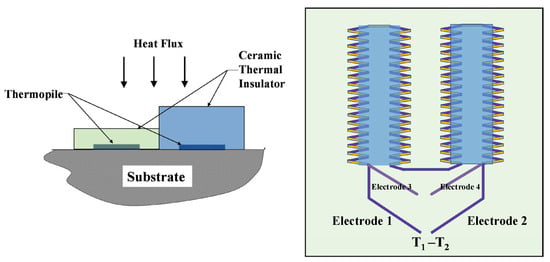
Figure 1. Schematic diagram of the principle of the composite thin-film thermoelectric sensor.

The fabricated TFHFs sample prepared by magnetron sputtering is shown in Figure 2. Under scanning electron microscopy (SEM), several interconnected thermopile strips exhibit dense and intact connections, with a minimum line width of 50 μm. Microscopic characterization of the cross-section indicates that the deposited Pt/PtRh13 thermopile sensitive film has a thickness of 310.6 nm, and the thermal resistance layer has a thickness of 2.482 μm, which are in good agreement with the design parameters.

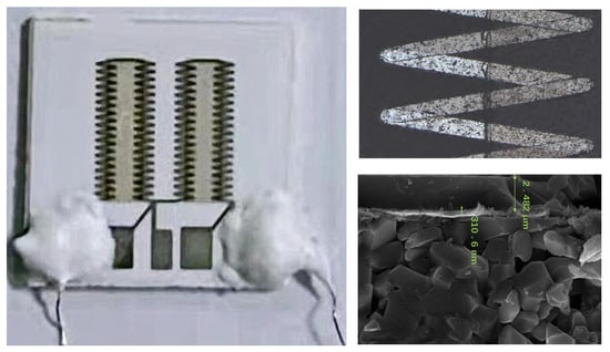
Figure 2. Fabricated TFHFs sample and SEM characterization results.

3. Simulation Study on Dynamic Response of TFHFs Under Different Thermal Boundary Conditions

3.1. Simulation of Heat Flux Dynamic Response Under Thermal Radiation Boundary

A finite element model of the TFHFs was established using COMSOL Multiphysics 6.1. The initial ambient temperature was set to 20 °C. A heat flux boundary was applied to simulate the laser-induced thermal excitation on the thin-film heat flux sensor, while considering heat dissipation through natural air convection and surface radiation. One-way coupling between solid heat transfer and the electric current interface was achieved via the thermoelectric effect. Figure 3 shows the three-dimensional temperature distribution of the thin-film heat flux sensor under thermal equilibrium under the above conditions, and Figure 4 presents the corresponding electric potential distribution of the thermopile. To validate the thermoelectric coupling functionality of the model, domain point probes were used to record the step heat flux response of both a single thermocouple and a complete thermopile. The simulation results (Figure 5) indicate that the peak and steady-state thermoelectric voltages of the two configurations exhibit approximately a four-fold relationship, confirming the effectiveness of the thermoelectric coupling in the model.

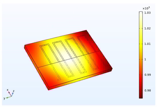
Figure 3. Simulated temperature distribution of the thin-film heat flux sensor.

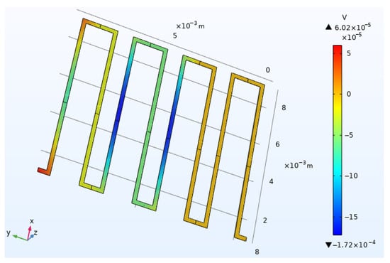
Figure 4. Simulated thermoelectric potential distribution of the thin-film heat flux sensor.

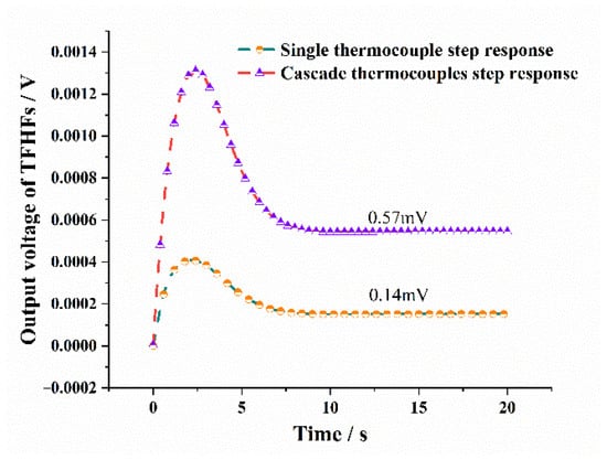
Figure 5. Simulated step response of a single thermocouple versus the cascade thermopiles under temperature difference excitation.

To further analyze the influence of substrate heat transfer on the step response of the thin-film heat flux sensor, thermally conductive materials with different thermal conductivity values were used to simulate a large turbine blade. The dynamic response characteristics of the sensor were investigated through simulation. As shown in Figure 6a, the thin-film heat flux sensor was closely attached to the surface of a 50 mm cubic heat sink. The materials of the heat sink were set as copper, iron, and alumina, with sequentially decreasing thermal conductivity. Under the same heat flux excitation, the step response curves of the TFHFs are shown in Figure 6b.

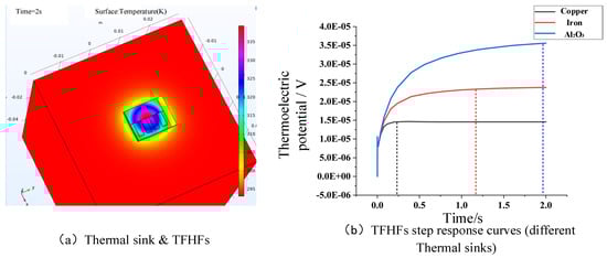
Figure 6. Dynamic response of TFHFs with different heat sink materials.

Based on the simulation results and with reference to Figure 5 and previous research findings [16], it can be concluded that the steady-state error in the step response of the TFHFs—caused by overshoot—stems from the poor thermal conductivity of the substrate, which deviates from ideal one-dimensional longitudinal heat conduction. When the sensor is attached to a heat sink with high thermal conductivity, heat accumulation within the substrate is effectively reduced. The auxiliary heat dissipation provided by the heat sink is significantly more efficient than natural convection in still air at room temperature, enabling the sensor to reach a step steady state more rapidly. Thus, under prolonged laser step excitation, the heat sink mitigates the hindering effect of the substrate on vertical heat transfer and reduces lateral heat spread from the hot to the cold end of the TFHFs, thereby decreasing the steady-state error during step-heat-flux calibration and measurement. Consequently, provided the heat sink offers sufficiently high thermal conductivity, the heat flux response of the TFHFs will closely approximate the analytical solution for the dynamic response of resistive film heat flux sensors, as expressed in Equation (1) [17].

$$\Delta T=T_1-T_2={\displaystyle \frac{2q_0\sqrt{at/\pi }}{\lambda }}\left[1-\exp (-{\displaystyle \frac{x^2}{4at}})\right]+{\displaystyle \frac{q_{0}x}{\lambda }}erfc({\displaystyle \frac{x}{2\sqrt{at}}}).$$

(1)

Here, $q_0$ represents the laser radiation heat flux, x represents the thickness of the thermal resistance layer, a represents the thermal diffusion coefficient of the thermal resistance layer, and $erfc$ represents the error complementary function. When the loaded laser radiation heat flux, the sensor structure, and the thermal property parameters are known, the dynamic response curve of this sensor can be obtained.

3.2. Simulation of Heat Flux Dynamic Response Under Thermal Convection Boundary

Previous studies have primarily focused on analyzing the dynamic response of TFHFs under thermal radiation boundaries. However, existing literature has demonstrated that different heat transfer modes significantly influence the sensor’s response during dynamic testing. It is therefore essential to conduct dynamic simulations of the thin-film heat flux sensor under high-temperature gas flow impact [18].

A two-dimensional dynamic simulation model was established to analyze the effects of high-temperature gas flow velocity and temperature on the dynamic response of the TFHFs’ heat flux component. The transient model was developed to simulate the dynamic thermal response of a heat flux sensor under a low-velocity air jet. The corresponding Reynolds number was in the low-turbulent or high-laminar regime. Given the low subsonic Mach number (<0.01), the flow was treated as incompressible. A laminar flow interface or a transition SST model was employed to accurately capture the near-wall heat transfer. A conjugate heat transfer analysis with a sufficiently refined mesh and small time steps was used to resolve the sensor’s transient response.

The sensor was placed in a high-temperature jet flow field with an initial temperature set to 293.15 K and an initial velocity of 0 m/s. The channel walls were adiabatic. The sensor was subjected to vertical convective heating and surface radiation to the environment. A Conjugate Heat Transfer interface was used to couple the Laminar Flow and Heat Transfer in Solids and Fluids interfaces. The temperature difference between the hot and cold electrodes of the sensor was the focus of the study. Two-point probes were placed at these electrodes to monitor the instantaneous value of $T_1-T_2$. Simulations were conducted under different fluid velocities u and temperatures $T_f$ to investigate their influence on the dynamic response (temperature difference). The typical flow velocity distribution is shown in Figure 7, and the heat transfer process between the high-temperature flow and the sensor at different time instances is illustrated in Figure 8.

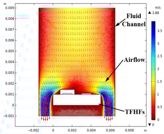
Figure 7. Simulated flow field distribution.

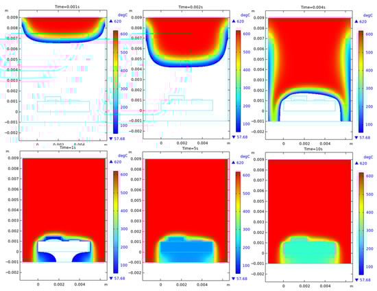
Figure 8. Simulated transient evolution of the temperature field.

Simulation results under different gas temperatures are shown in Figure 9a. When the inflow velocity was set to 2 m/s with temperatures of 200 °C, 300 °C, 400 °C, and 500 °C, the step response amplitude of the thin-film heat flux sensor increased proportionally with the gas temperature. However, the effect of gas temperature on the time constant of the TFHFs was limited, with no clear trend observed. As illustrated in Figure 9b, when the gas temperature was set to 300 °C with inflow velocities of 0.5 m/s, 1 m/s, 2 m/s, and 3 m/s, the time constant decreased with increasing flow velocity. This correlation is consistent with empirical correlations for gas turbulent flow and convective heat transfer coefficients, as expressed in Equation (2) [19].

$$h=0.023{({\displaystyle \frac{ud}{v}})}^{0.8}{\mathrm{Pr}}^{0.4}{\displaystyle \frac{k}{L}}$$

(2)

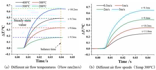
Figure 9. Dynamic simulation results of TFHFs’ heat flux under different flow field parameters.

In the equation, $h$ represents the convective heat transfer coefficient; u, the flow velocity; ν, the kinematic viscosity; $d$, the pipe diameter; Pr, the Prandtl number; $k$, the thermal conductivity of the flow; and L, the characteristic size of the test section. During the initial stage of the TFHFs’ heat flux response, the temperature difference $\Delta T=T_1-T_2$—which is proportional to the measured heat flux—is mainly governed by the temperature increase at the hot electrode. Due to the thermal insulation provided by the resistance layer, the cold electrode remains close to the initial temperature of 293.15 K, resulting in $d{T}_2/dt\approx 0$. Therefore, the rate of change in the heat flux (temperature difference), $d(T_1-T_2)/dt\approx d{T}_1/dt$, indicates that the initial rise rate of the response curve is primarily determined by the hot electrode. This interpretation is corroborated by the simulated temperature profiles of the cold and hot electrodes, as shown in Figure 10.

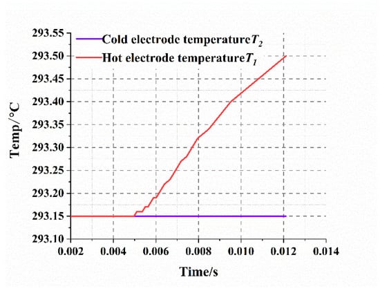
Figure 10. Temperature variation at the cold and hot electrodes of the thin-film heat flux sensor.

Therefore, within this time period, the dynamic response rate of the thin-film heat flux sensor can be represented by the temperature rise rate at the hot electrode, focusing on its time constant $\tau$. According to the lumped parameter model, the simplified expression of the hot electrode in the flow field is given as:

$$\rho cV{\displaystyle \frac{d{T}_1}{dt}}=-hS(T_f-T_1)$$

(3)

where $c$ is the specific heat capacity of the hot electrode material, $\rho$ is its density, $V$ is the volume of the hot electrode, $T_1$ is the instantaneous temperature of the hot electrode, $T_f$ is the fluid temperature, $h$ is the convective heat transfer coefficient, $S$ is the surface area of the hot electrode, and $t$ is time. Solving the above differential equation yields:

$$T_1-T_0=(T_f-T_0)(1-e^{-{\displaystyle \frac{hS}{c\rho V}}t})$$

(4)

The time constant τ of the hot electrode is defined as the time required for the temperature difference between the measured temperature $T_1$ and the initial temperature $T_0$ to reach 63.2% of the total step change $T_f-T_0$. In practical calibration experiments, τ can be obtained by calculating the time interval between the initial temperature $T_0$, the final steady-state temperature $T_f$, and the intermediate temperature point $T_0+(T_f-T_0)\times 63.2\%$. However, this method relies solely on a single instantaneous temperature value, making it highly susceptible to experimental noise and interference, thereby resulting in low reliability. By applying the Z-transform and taking the logarithm, the following expression is derived:

$$\ln (1-{\displaystyle \frac{T_1-T_0}{T_f-T_0}})=-{\displaystyle \frac{hS}{c\rho V}}t=-{\displaystyle \frac{t}{\tau }}$$

(5)

The time constant can be determined by performing linear fitting to calculate the slope. Substituting Equation (2) into Equation (5) yields:

$$\tau \propto {\displaystyle \frac{c}{u^{0.8}}}$$

(6)

Thus, the flow velocity u is negatively correlated with the time constant $\tau$ of the hot electrode, but positively correlated with its temperature rise rate, as expressed in Equation (7). Consequently, during the initial stage of the TFHFs’ heat flux response, higher flow velocities result in a steeper response curve and a shorter time constant.

$$u\uparrow \Rightarrow d{T}_1/dt\uparrow \Rightarrow d(T_1-T_2)/dt\uparrow \Rightarrow \tau \downarrow$$

(7)

In summary, the dynamic characteristics of the thin-film heat flux sensor under high-temperature gas flow impact are predominantly influenced by the flow velocity. Furthermore, it is not difficult to observe from Formula (5) that the higher the convective heat transfer coefficient is, the smaller the time constant of the sensor will be. It is indicated that in turbulent conditions, the sensor can achieve a faster response speed compared to laminar flow. To accurately determine the dynamic behavior of the sensor under convective boundary conditions, the flow velocity and laminar/turbulent state of the fluid layer provided by the calibration device must match the actual application scenario; otherwise, significant errors may occur in the calibration results.

3.3. Simulation of TFHFs Temperature Dynamic Characteristics Under Type-I Thermal Boundary (High-Temperature Furnace)

To compare the dynamic response characteristics of the TFHFs’ temperature measurement component under different heat transfer conditions, a multiphysics thermoelectric model was established using finite element analysis. The fast-response thermocouple consists of a sensing junction and positive/negative thermoelement wires, both made of platinum-rhodium noble metal, corresponding to a Type S thermocouple.

To simulate the heat transfer conditions during the dynamic calibration of the thermocouple in a high-temperature furnace, the thermoelectric effect multiphysics coupling module in COMSOL was employed. The time error introduced by the thermocouple ejection device during dynamic calibration was neglected. A step function was applied to impose a dynamic temperature excitation of 1273.15 K on the sensing junction. Based on empirical values, the convective heat transfer coefficient between the sensing junction and the furnace air was set to $h$ = 15 W/(m²⋅K), and the ambient temperature $T_{ext}$ was set to 1273.15 K. Radiation heat transfer occurred between the sensing junction and the furnace wall, with the inner wall temperature $T_w$ set to 1323.15 K and the surface emissivity $\epsilon$ of the sensing junction set to 0.13. The positive and negative thermoelement wires, located outside the furnace, experienced natural convection with the laboratory environment, with a heat transfer coefficient of 10 W/(m²·K) and an ambient temperature of 293.15 K. Heat conduction between the thermoelement wires and the sensing junction raised the wire temperatures, and radiation heat dissipation occurred with the laboratory environment, with an emissivity of 0.13 and an ambient temperature of 293.15 K.

After completing the calculation with the above simulation parameters, the three-dimensional temperature distribution and the thermoelectric potential response curve of the thermocouple model at steady state are shown in Figure 11a and Figure 11b, respectively. The calculated time constant of the thermocouple model under ideal high-temperature furnace dynamic calibration conditions is 44.8 μs.

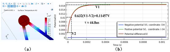
Figure 11. Dynamic simulation results of the TFHFs thermocouple under a type I thermal boundary.

As observed in Figure 11b, the sensing junction of the thermocouple reaches dynamic equilibrium within 200 μs. Within such a short duration, the amount of heat transferred from the junction to the thermoelement wires is negligible, resulting in low temperatures along the entire length of the wires, as shown in Figure 11a. The results indicate that as the furnace temperature increases from 1273 K to 1873 K, the time constant of the thermocouple gradually decreases. This finding is consistent with experimental trends reported in previous studies by other researchers, demonstrating that the boundary conditions set in this finite element simulation model are reasonable. The model effectively replicates the ideal environment for dynamic calibration of thermocouples under type I thermal boundary conditions, and the conclusions are reliable.

3.4. Simulation of TFHFs Temperature Dynamic Characteristics Under Type II Thermal Boundary (Laser)

In contrast to the Type I thermal boundary described in Section 3.3, step laser heating of the thermocouple constitutes a Type II thermal boundary (constant power density). Using the same thermocouple model, simulations were conducted under heat transfer conditions strictly consistent with step laser-based dynamic testing. Parameters related to radiation and convective heat exchange between the sensing junction, thermoelement wires, and the environment remained unchanged. Theoretical calculations and repeated adjustments of excitation parameters confirmed that a laser power of 0.5 W results in a step steady-state temperature of 1273.15 K at the thermocouple. Excessive power would cause heat absorption at the junction to far exceed heat dissipation, leading to rapid temperature rise beyond the melting point of the wires. Under the above conditions, the three-dimensional temperature distribution and thermoelectric potential response curve of the thermocouple model at steady state are shown in Figure 12a and Figure 12b, respectively.

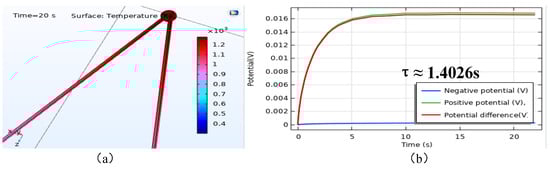
Figure 12. Dynamic simulation results of the TFHFs thermocouple under a Type II thermal boundary.

Simulation results indicate that to achieve the same steady-state temperature of 1273 K, the time constant of the thermocouple under ideal laser-based (Type II thermal boundary) dynamic calibration is 1.4026 s, and the output response stabilizes only after 10 s. Furthermore, comparing Figure 11a and Figure 12a reveals that when the thermocouple sensing junction reaches the same temperature under thermal equilibrium, laser heating causes a more significant temperature increase along the thermoelement wires. Nearly two-thirds of the wire length near the junction exceeds 1000 K, and the temperature difference between the sensing junction and distant wire measurement points is relatively small. This is attributed to the prolonged duration of laser heating, which allows continuous heat transfer from the sensing junction to the wires while energy is being absorbed.

It can be concluded that in the dynamic calibration of wire-type thermocouples, the heat transfer conditions significantly influence the time constant. Under step laser heating, the thermocouple response struggles to reach an ideal steady state, and heat accumulation at the junction under constant optical power intensifies, easily exceeding the melting point. Moreover, both simulations and experiments show that achieving dynamic calibration at a specified temperature using laser excitation requires pre-adjustment or theoretical calculation of the laser power, resulting in low calibration efficiency. In summary, when employing laser-based step heating for dynamic calibration, it is necessary to incorporate a laser power feedback control module to adjust the power in real time, enabling the thermocouple to rapidly reach and maintain the target temperature.

4. TFHFs Dynamic Testing Experiment

4.1. Dynamic Heat Flux Testing of TFHFs Under Thermal Radiation Boundary

The fabricated ceramic-based TFHFs sample was dynamically tested using the constructed high-precision laser thermal radiation dynamic calibration system. The laser power P was set to 600 W with a spot radius of 8 mm, resulting in a calculated heat flux density of 3 MW/m². A step voltage signal modulated by an analog signal generator was used to drive the laser output. When the heat flux step response of the TFHFs reached a steady state, the step response amplitude $\Delta A$ was recorded, the steady-state response time $T_r$ was calculated, and the step heat flux excitation signal captured by a high-speed photodetector was simultaneously collected. Based on the finite element simulation results of the step response in Section 3.1, it is known that adding a heat sink with high thermal conductivity helps the thin-film heat flux sensor achieve step steady-state more quickly while reducing steady-state errors caused by overshoot. Therefore, a large cubic copper heat sink was designed, which is a piece of copper block with extremely high thermal conductivity, with a side length of 8 cm. Its thermal conductivity is approximately 398 W/(m·K), which is much higher than that of the film sample. Therefore, in transient heat conduction, it can be regarded as a semi-infinite body. And the TFHFs were tightly attached to its surface using thermal conductive adhesive, as shown in Figure 13a. The thickness of the used thermal conductive silicone is 0.8 mm, and its thermal conductivity reaches 4.0 W/(m·K). The heat flux response signal and laser excitation signal collected under the above experimental conditions are presented in Figure 13b.

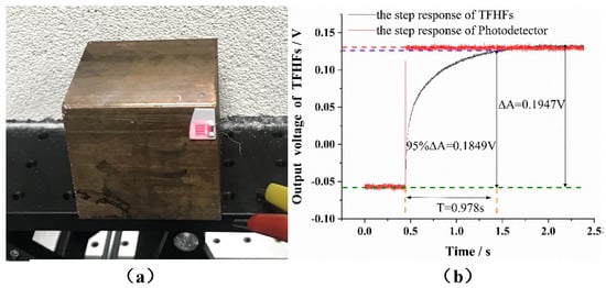
Figure 13. Dynamic step response test results of TFHFs with a heat sink.

Before the experiment, the surface of the sample was coated with a high-temperature-resistant blackbody paint with an emissivity of 0.95. When the surface of the thin film sample was heated to its maximum temperature (approximately 1100 °C, as monitored by an infrared radiation thermometer), according to the Stefan-Boltzmann law, the amount of radiation and heat dissipation $q_{rad}$ from the sample to the surrounding environment was approximately 1.91 × 10⁵ W/m². When the external environment temperature was at room temperature and the natural convective heat transfer coefficient h = 15 W/(m²·K), the convective heat loss $q_{\mathrm{cov}}$ was approximately 1.61 × 10⁴ W/m². Therefore, the heat loss rate in the experiment was approximately 6.9%.

The experimental curve indicates that the rising edge of the excitation signal measured by the photodetector closely approximates an ideal step signal. After signal amplification, the response amplitude $\Delta A$ of the TFHFs was 0.1947 V, and the response time $T_r\prime$ was 0.978 s, which is of the same order of magnitude as the finite element simulation result of 1.125 s from Section 3.1. However, it is significantly larger than the result (98 μs) calculated by the numerical model described in Equation (1). This discrepancy arises because the numerical model is based on the assumption of one-dimensional unidirectional heat transfer in a semi-infinite medium, whereas the TFHFs are deposited on a substrate material and do not exhibit ideal one-dimensional heat conduction. Particularly at high temperatures, thermal physical parameters such as the thermal conductivity $\lambda$ of the thin film undergo changes. Additionally, the sensor features a multilayer thin-film structure, where interlayer thermal resistance and the influence of the alumina protective layer play significant roles.

It is important to note that under the excitation of ultrafast lasers on the thin film, non-Fourier effects may occur. However, this experiment is within the range where the classical model is fully applicable [20,21].

In the frequency domain measurement of TFHFs, the sensors were tested using two periodic square-wave laser excitations at different frequencies. This approach leverages the harmonic properties of the periodic square waves and the principles of the Fourier transformation. The frequencies used are 100 Hz and 200 Hz. The amplitude-frequency characteristic curve of the TFHFs obtained from the experiment is shown in Figure 14. From this, it can be determined that the −3 dB cutoff frequency of this thin-film thermal flow sensor is within the range of 3000 to 3100 Hz.

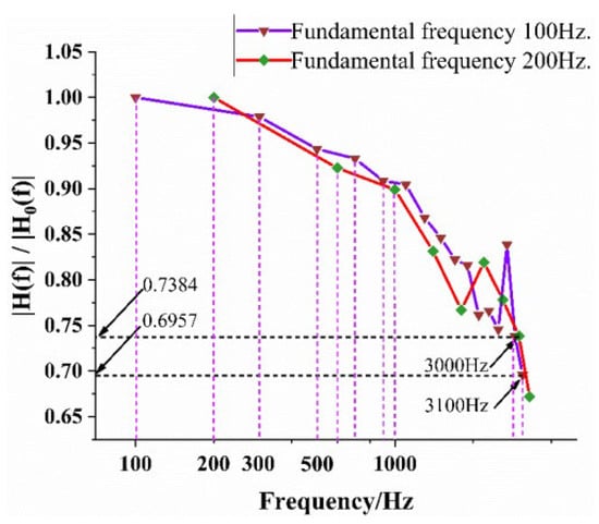
Figure 14. Measurement of the upper cutoff frequency of TFHFs.

4.2. Dynamic Heat Flux Testing of TFHFs Under Thermal Convection Boundary

The experimental setup for the high-temperature wind tunnel heat flux test is shown in Figure 15. Before the test, the TFHFs sample and a standard Gardon gauge were mounted together on the same fixture. During the experiment, after the flow parameters (such as gas temperature and Mach number) reached a steady state, the fixture was inserted into the flow, and the output thermoelectric signals of both heat flux sensors were recorded simultaneously. Based on the simulation results from Section 3.2, this wind tunnel test focused on the dynamic characteristics of the TFHFs sample under a fixed flow temperature (1000 °C) and varying Mach numbers.

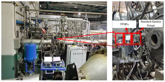
Figure 15. High-temperature wind tunnel heat flux test site.

The data measured by the TFHFs and the standard Gardon gauge in the first test are shown in Figure 16. It is necessary to emphasize that the initial position of the blade is 1.2 m away from the high-temperature zone in the horizontal direction. During the test, a mechanical translation device was used to push the blade fixture into the flow field at a constant velocity. The average speed of this ejection device is 1 m per second. The data is fully recorded, including the preparation time before the ejection. However, the sensors began to output data at the 50,000th sampling point, and at this moment, the sample was exactly in the high-temperature area. The output voltages of both heat flux sensors increased rapidly and stabilized. To ensure the safety of the thin-film heat flux sample during the initial test, it was retracted from the heating zone ahead of the Gardon gauge once its output reached a preliminary steady state (at 130 s). Analyzing the data from the time interval of 115 s to 120 s, the steady-state heat flux values measured by the TFHFs sample and the standard Gardon gauge were 294 kW/m² and 301 kW/m², respectively, resulting in a measurement error of 2.3%. The peak heat flux values reached by both sensors were similar, approximately 330 kW/m². The thin-film heat flux sensor sample took about 70 s to reach the peak heat flux from its initial state.

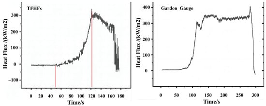
Figure 16. High-temperature wind tunnel test results (Ma: 0.5, Temperature: 1000 °C).

In the second test, the gas temperature in the wind tunnel remained unchanged at 1000 °C, while the flow velocity was increased to Mach 0.86. After the flow parameters stabilized, both heat flux sensors were inserted into the flow field following the same procedure. The heat flux curves measured by the TFHFs and the Gardon gauge are shown in Figure 17. Compared with the test results at 1000 °C and Mach 0.5, the rising edge of the TFHFs heat flux curve became steeper. The output heat flux values of both the standard Gardon gauge and the TFHFs sample decreased to some extent, which was intended to protect the sample and obtain more test data. Therefore, during the second test, as the fixture was moved to different positions in the flow field, the local heat flux density environment experienced by the sensors changed. At the 75 s mark, both the TFHFs sample and the standard Gardon gauge reached a stable heat transfer state. However, a significant error was observed between the heat flux values measured by the two sensors. This discrepancy is speculated to be due to sensitivity drift caused by surface damage to the sensors resulting from prolonged exposure to high-temperature gas flow.

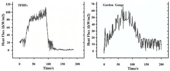
Figure 17. High-temperature wind tunnel test results (Ma: 0.86, Temperature: 1000 °C).

The two tests demonstrate that the designed TFHFs exhibit favorable dynamic heat flux performance and are capable of operating under extreme conditions of 1000 °C and high Mach numbers. The temporal-heat flux variation trend aligns well with that of the standard heat flux gauge. Furthermore, under convective heat transfer boundary conditions, an increase in flow velocity contributes to a faster response of the TFHFs, which is consistent with the simulation conclusions in Section 3.2. A noted limitation lies in the absence of an ideal ejection mechanism, as the conventional mechanical translation device used in the tests introduced a significant time delay.

4.3. Dynamic Temperature Testing of TFHFs Thermocouples Under Laser Thermal Radiation

Based on the aforementioned laser thermal radiation dynamic test platform, a 6 kW high-power fiber-output semiconductor laser was used as the thermal excitation source, with the surface temperature of the calibrated TFHFs thin-film temperature sensor as the controlled variable. The control system aims to maintain the difference between the sensor’s temperature and the set temperature within an acceptable range. A high-speed infrared radiation thermometer serves as the feedback measurement unit, acquiring the surface temperature of the calibrated thin-film thermocouple and relaying the data to the system input for comparison with the reference value. A high-precision data acquisition card acts as the controller, employing a custom LabVIEW program to collect temperature signals from the infrared thermometer. The deviation between the measured and set temperatures is processed by a fuzzy adaptive PID control algorithm to compute the control signal. The acquisition card then outputs a corresponding 0–10 V DC control voltage to the laser, thereby regulating its output energy.

This constant temperature control system employs a Fuzzy-PID controller. The fuzzy logic, with a compact 5 × 5 rule base and triangular membership functions, handles coarse, nonlinear adjustments, while the PID fine-tunes the response. The update cycle is 10 ms, with a total loop delay under 15 ms. A thermocouple provides feedback, filtered by a moving average or a low-pass digital filter (cutoff ~1 Hz) to mitigate noise. The setpoint uses a gradual ramp to minimize overshoot. Output saturation (e.g., 0–10 V) is managed with an anti-windup scheme in the PID. The controller is tuned via the Ziegler-Nichols method. Key reported metrics are rise time, overshoot, settling time, and steady-state error.

The system schematic is shown in Figure 18, and the improved dynamic test platform for laser-based thermal radiation testing of composite thermoelectric devices is illustrated in Figure 19.

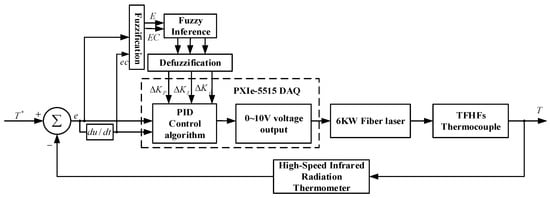
Figure 18. Schematic of constant temperature feedback control for a thermocouple.

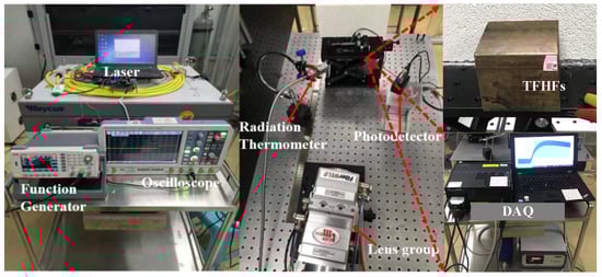
Figure 19. Dynamic test platform for laser thermal radiation of composite thermoelectric devices.

On the LabVIEW host computer interface, the laser power was set to 40% (corresponding to a 4 V analog voltage input and approximately 2300 W), 30% (3 V analog voltage input, ~1650 W), and 20% (2 V analog voltage input, ~1000 W). Under external/continuous operation mode, dynamic testing of the TFHFs thermocouple was performed using an open-loop step laser without feedback. The resulting step temperature response curves are shown in Figure 20.

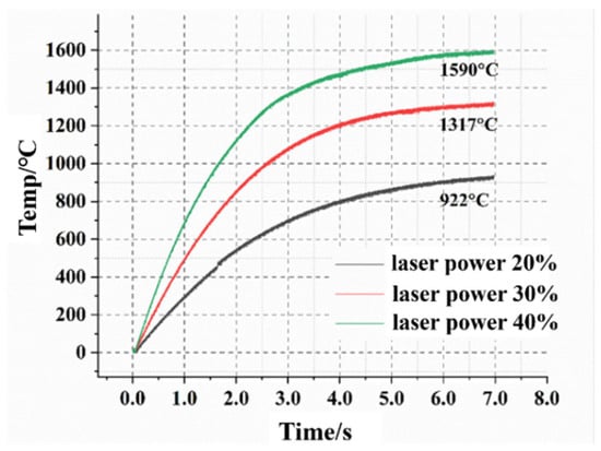
Figure 20. Laser dynamic test experiment of TFHFs thermocouple (without feedback).

The experimental results indicate that when the laser beam heats the thermocouple, the output thermoelectric potential initially rises sharply in an exponential manner. As the temperature of the thermocouple continues to increase, heat transfer from the sensing junction to the thermoelement wires intensifies. When the heat capacity of the junction and the wires approaches saturation, the response curve begins to increase slowly in a logarithmic form. The entire process lasts on the order of seconds. At the 7 s mark, the thermocouple temperatures reached 1590 °C, 1317 °C, and 922 °C, respectively. However, the output continued to show an upward trend, making it difficult to reach a step steady state and preventing an accurate evaluation of the thermocouple’s time constant. This confirms that step laser excitation does not serve as an ideal temperature step excitation signal, a conclusion consistent with the simulation results in Section 3.4.

The above open-loop experiments demonstrate that when heating the thermocouple with a laser whose power changes in a stepwise manner, the response curve continues to rise. Therefore, it is necessary to achieve a temperature step excitation through closed-loop constant temperature feedback control of the laser. In the feedback test experiments, the laser power was set constant at 40%, while the threshold voltages were set to 2.2 V, 2.5 V, 2.8 V, and 3 V, respectively. Taking the threshold of 2.8 V (corresponding to a steady-state temperature of 1235 °C) as an example, the voltage feedback from the infrared radiation thermometer (which has a linear relationship with the measured surface temperature of the thermocouple and serves as the input signal to the controller) and the output laser control voltage curve from the feedback controller are shown in Figure 21.

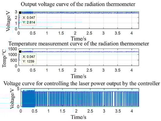
Figure 21. Input and output signals of the feedback controller (laser power: 40%, threshold: 2.8 V).

Under the four different threshold parameter settings described above, the step response curves of the TFHFs thermocouple are shown in Figure 22. Compared with the open-loop test curves in Figure 20, it is observed that after incorporating feedback control into the calibration platform, the thermocouple can rapidly reach the target temperature and maintain a near-ideal steady state. This demonstrates that the constant-temperature feedback control module designed in this work can achieve dynamic calibration at arbitrary temperatures by setting the threshold voltage (temperature), while maintaining a nearly ideal step steady state. This approach resolves the issue in traditional step-laser dynamic testing of thermocouples, where achieving an ideal steady state is difficult, thereby preventing accurate calculation of the time constant. It also compensates for the inherent theoretical limitations of using step laser excitation as a dynamic thermal excitation source under certain thermal boundary conditions, as discussed in Section 3.4.

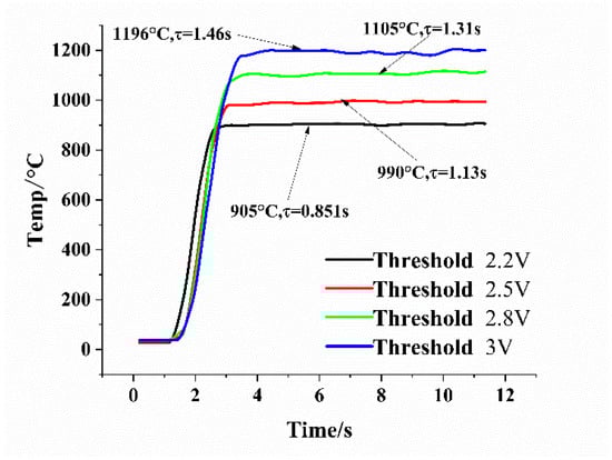
Figure 22. Laser dynamic test results of TFHFs thermocouples at different threshold temperatures (with feedback).

Taking the multiple repeatability tests with a threshold voltage of 2.2 V as an example, the 5 test data under the same experimental conditions are shown in Table 1. According to the repeatability error evaluation method, the repeatability error of the thermocouple time constant calibration can be calculated to be 0.91%.

Table 1. Time constant repeatability test data of thermocouple.

Number of Experiments	1	2	3	4	5
τ (ms)	845	843	855	849	862

Regarding the test results that relied on a laser as the heat source, when combined with the repeatability test data of thermocouple time constants shown in Table 1, it indicates that the average value is 850.8 ms. Due to the limited number of measurements, the experimental standard deviation S_k = R/C = 8.15 ms. Here, R represents the range of the 5 measurement values, and C is the corresponding range coefficient. When the number of experiments n = 5, the coefficient of range C is 2.33. Then, the A-class uncertainty of the measured result can be calculated using the following formula.

$$u_A(\overline{\tau })={\displaystyle \frac{S_k}{\sqrt{n}}}={\displaystyle \frac{R}{C\sqrt{n}}}=2.24\mathrm{m}\mathrm{s}$$

(8)

Since the time constant is read as the difference between two time points from the response signal, the estimated value of the measured response time is uniformly distributed within the interval. The sampling frequency set by the acquisition device is 20 MHz. Through the Formula (9), the B-type uncertainty of the estimated value ts of the measured response time can be obtained, where k is the confidence factor. When it is uniformly distributed, $k=\sqrt{3}$.

$$u_B(\overline{\tau })={\displaystyle \frac{\Delta t}{k}}=0.00000005/\sqrt{3}=0.0289\mathsf{\mu }\mathrm{s}$$

(9)

Therefore, the calculation of the combined standard uncertainty $u_C(\overline{\tau })$ is as follows:

$$u_C(\overline{\tau })=\sqrt{{\displaystyle {\sum }_{i=1}^N{u}_i^2(\tau )}}=\sqrt{u_A^2+u_B^2}\approx 2.24\mathrm{m}\mathrm{s}$$

(10)

The expanded uncertainty $U$ is:

$$U=k{U}_C=4.48\mathrm{m}\mathrm{s}$$

(11)

In the usual measurement, the inclusion factor k is generally taken as 2. The expanded uncertainty is 4.48 ms, the time constant τ is (850.8 ± 4.48) ms.

5. Conclusions

To address the high-transient and multi-thermal-boundary conditions of aero-engine turbine blades, this study designed a TFHFs integrated heat flux and temperature thin-film thermoelectric sensor. A laser-based thermal radiation dynamic test platform for composite thermoelectric devices was developed, with a focus on investigating the dynamic characteristics of the sensor under multiple thermal loading conditions. The main conclusions and innovations are as follows:

(1) In the dynamic testing of radiative heat flux in TFHFs, a multi-physics finite element modeling and simulation approach was innovatively combined with laser thermal radiation experiments to demonstrate that overshoot in the heat flux step response originates from non-ideal longitudinal heat conduction. This phenomenon was mitigated through the use of a heat sink.

(2) In the dynamic testing of convective heat flux in TFHFs, two-dimensional non-isothermal flow CFD simulations and theoretical modeling of the transient heat flux response clarified that the dynamic behavior of the device is primarily influenced by flow velocity. This conclusion was validated through high-temperature wind tunnel experiments.

(3) In the dynamic temperature testing of TFHFs, the intrinsic differences in step response mechanisms under Type I and Type II thermal boundaries were innovatively analyzed through simulation. It was confirmed that the thermocouple response under step laser heating struggles to achieve ideal stability. To address this, a laser thermal radiation dynamic test platform for composite thermoelectric devices, centered around a laser power feedback controller, was designed and implemented. This platform enables efficient step dynamic testing of TFHFs thermocouples at arbitrary steady-state temperatures.

However, the laser feedback control module adopted in this work is only applicable when the thermocouple nodes are relatively large. Otherwise, the high-speed infrared radiation thermometer will be unable to focus on and measure the temperature of the nodes, nor will it be able to provide feedback. This aspect requires further improvement in the later stage.

References

- Yoshida, M.; Nakamura, H.; Yamada, S.; Funami, Y. High spatiotemporal resolution measurement of water flow boiling heat transfer in a horizontal square minichannel using infrared thermography. Int. J. Heat Mass Transf. 2025, 238, 126457. [Google Scholar] [CrossRef]
- Bohn, D.; Heuer, T.; Kortmann, J. Numerical conjugate flow and heat transfer investigation of a transonic convection-cooled turbine guide vane with stress-adapted thicknesses of different thermal barrier coatings. In Proceedings of the 38th Aerospace Sciences Meeting and Exhibit, Reno, NV, USA, 10–13 January 2000. [Google Scholar] [CrossRef]
- Azzi, A.; Jubran, B.A. Influence of leading-edge lateral injection angles on the film cooling effectiveness of a gas turbine blade. Heat Mass Transf. 2004, 40, 501–508. [Google Scholar] [CrossRef]
- Guo, H.; Jiang, J.Y.; Liu, J.X.; Nie, Z.H.; Ye, F.; Ma, C.F. Fabrication and Calibration of Cu-Ni Thin Film Thermocouples. Adv. Mater. Res. 2012, 512–515, 2068–2071. [Google Scholar] [CrossRef]
- Ran, L. Research and Realization of Convergence Between Infrared Temperature Measurement Technology and Video Surveillance System of Substation. Power Syst. Technol. 2008, 32, 80–82. [Google Scholar]
- Serio, B.; Nika, P.; Prenel, J.P. Static and dynamic calibration of thin-film thermocouples by means of a laser modulation technique. Rev. Sci. Instrum. 2000, 71, 4306–4313. [Google Scholar] [CrossRef]
- DiDomizio, M.J.; Dehghani, P. Measuring two-dimensional heat flux using a plate sensor and infrared thermography. MethodsX 2025, 14, 103327. [Google Scholar] [CrossRef] [PubMed]
- Li, Z.; Wang, G.; Yin, J.; Xue, H.; Guo, J.; Wang, Y.; Huang, M. Development and performance analysis of an atomic layer thermopile sensor for composite heat flux testing in an explosive environment. Electronics 2023, 12, 3582. [Google Scholar] [CrossRef]
- Cheng, L.; Dong, H.; Tang, L.; Tan, Q.; Xiong, J. Dynamic characterization measurement of the circular foil heat flux sensor based on laser method. Opt. Lasers Eng. 2025, 184, 108642. [Google Scholar] [CrossRef]
- Imaeda, H.; Toida, R.; Takeuchi, T.; Awano, H.; Tanabe, K. Significant improvement in sensitivity of an anomalous Nernst effect–based heat flux sensor by composite structure. arXiv 2025, arXiv:2405.07758. [Google Scholar]
- Brune, J.E.; Sander, T.; Rödiger, T.; Huber, K.; Mundt, C. Experimental investigation of atomic layer thermopile heat-flux sensors in a shock tube. In Proceedings of the AIAA SciTech Forum 2023, National Harbor, MD, USA, 23–27 January 2023; p. 2263. [Google Scholar]
- Chen, X.; Tao, B.W.; Zhao, R.P.; Yang, K.; Li, Z.Z.; Xie, T.; Zhong, Y.; Zhang, T.; Xia, Y.D. The atomic layer thermopile heat flux sensor based on the inclined epitaxial YBa2Cu3O7-δ films. Mater. Lett. 2023, 330, 133336. [Google Scholar] [CrossRef]
- Liu, F.; Cai, X.; Cai, T. Inverse transfer function identification for high-frequency pressure probes using M-sequence pressure generators. Flow Meas. Instrum. 2022, 87, 102221. [Google Scholar] [CrossRef]
- Rau, G.C.; Andersen, M.S.; Acworth, R.I. Experimental investigation of the thermal time-series method for surface water-groundwater interactions. Water Resour. Res. 2012, 48, 1115–1118. [Google Scholar] [CrossRef]
- Lopardo, G.; Bertiglia, F.; Curci, S.; Roggero, G.; Merlone, A. Comparative analysis of the influence of solar radiation screen ageing on temperature measurements by means of weather stations. Int. J. Climatol. 2014, 34, 1297–1310. [Google Scholar] [CrossRef]
- Zhang, C.; Huang, J.; Li, J.; Yang, S.; Ding, G.; Dong, W. Design, fabrication and characterization of high temperature thin film heat flux sensors. Microelectron. Eng. 2019, 217, 111128. [Google Scholar] [CrossRef]
- Tao, W.Q. Heat Transfer, 4th ed.; Higher Education Press: Beijing, China, 2006. [Google Scholar]
- Amarante, A.; Lanoiselle, J.L. Heat transfer coefficients measurement in industrial freezing equipment by using heat flux sensors. J. Food Eng. 2005, 66, 377–386. [Google Scholar] [CrossRef]
- Bergman, T.L.; Lavine, A.S.; Incropera, F.P.; Dewitt, D.P. Fundamentals of Heat and Mass Transfer, 7th ed.; John Wiley & Sons: Hoboken, NJ, USA, 2013. [Google Scholar]
- Mao, Y.; Xu, M. Non-Fourier heat conduction in a thin gold film heated by an ultra-fast laser. Sci. China Technol. Sci. 2015, 58, 638–649. [Google Scholar] [CrossRef]
- Raveshi, M.R. Non-Fourier heat conduction in an exponentially graded slab. J. Appl. Mech. Tech. Phys. 2016, 57, 326–336. [Google Scholar] [CrossRef]
Disclaimer/Publisher’s Note: The statements, opinions and data contained in all publications are solely those of the individual author(s) and contributor(s) and not of MDPI and/or the editor(s). MDPI and/or the editor(s) disclaim responsibility for any injury to people or property resulting from any ideas, methods, instructions or products referred to in the content. |
© 2025 by the authors. Licensee MDPI, Basel, Switzerland. This article is an open access article distributed under the terms and conditions of the Creative Commons Attribution (CC BY) license (https://creativecommons.org/licenses/by/4.0/).