A Novel Execution Time Prediction Scheme for Efficient Physical AI Resource Management

Abstract

Physical AI enables reliable and timely operations of autonomous systems such as robots and smart manufacturing equipment under diverse and dynamic execution environments. In these environments, computing resources are often limited, shared among tasks, and fluctuate over time. This makes it difficult to guarantee that tasks meet timing constraints. As a result, resource-aware execution time prediction becomes essential for efficient resource management in physical AI systems. However, existing methods typically assume specific environments or static resource usage and often fail to generalize to new environments. In this paper, we propose CARE-D (Calibration-Assisted Resource-aware Execution time prediction), which trains a deep neural network to model the nonlinear relationships among hardware characteristics, resource levels, and task features across environments. The model predicts the execution time of tasks under diverse hardware and dynamically allocated computing resources, using a few execution records from new environments. CARE-D applies few-history-based calibration using only 1 to k execution records from target environments to adjust predictions without retraining the model. Experiments show that CARE-D improves prediction accuracy by about 7.3% over zero-history predictors within a 10% relative error and outperforms regression and deep learning baselines, using only one to five records per target environment.

1. Introduction

Physical Artificial Intelligence (Physical AI) has become a key enabler of autonomous system operation, allowing robots, unmanned vehicles, and smart manufacturing equipment to operate reliably in real-world environments [1,2,3]. Physical AI workloads are deployed on various execution settings with diverse devices, dynamically allocated computing resources, and varying task characteristics [4,5,6]. In such environments, computing resources are often limited, shared among multiple tasks, and their available capacity fluctuates over time, so the execution time of physical AI tasks depends not only on model complexity, but also on environment-dependent factors. This environment-coupled execution time variability makes it difficult to guarantee stable performance and timely responses for safety-critical and time-sensitive operations [7,8]. Therefore, an accurate and resource-aware execution time prediction scheme is necessary to support reliable resource management across physical AI environments.

The execution time of a physical AI task can be regarded as a multivariate function of several groups of factors. It depends on task specific characteristics such as model architecture, FLOPs, and input or output tensor structures [9,10,11]. It is also affected by hardware-level attributes, including CPU family, microarchitectural behavior, and memory bandwidth [12,13], as well as dynamically assigned resource levels such as CPU resource levels, memory capacity, and I/O throughput. If this multivariate dependency is not modeled accurately, computing resources may be under allocated, causing deadline misses, execution delays, and reduced throughput, or over allocated, leading to wasted energy and lower overall system efficiency [14,15]. In time-critical physical AI applications such as manufacturing cells and robotic production lines, persistent errors in execution time estimation can further accumulate into mission failures, increased cycle time, or unstable operation in real-world environments.

Existing studies have explored execution time prediction in high-performance computing, cloud platforms, workflow systems, and GPU-based workloads. In high-performance and GPU computing domains, prior research has employed statistical regression and deep learning models to estimate kernel level runtime from hardware performance counters and instruction-level features extracted from job traces [16,17,18,19]. In distributed and cloud environments, machine learning-based regressors and resource utilization models have been applied to predict workload latency using CPU usage patterns, historical job profiles, and cluster-level resource metrics [20,21]. Workflow-oriented methods have incorporated recurrent neural networks and attention- or Transformer-based models to forecast completion time in multi-stage pipelines by modeling task dependencies and event sequences [22,23]. Together, these approaches demonstrate that data-driven models can provide accurate execution time prediction when sufficient execution history is available in relatively homogeneous and well provisioned computing clusters.

However, the previous works may face fundamental limitations when applied to physical AI systems. Most prior approaches assume static execution environments, fixed computing resource allocations, and abundant environment specific execution records, which makes it difficult for them to capture runtime variations caused by fluctuating resource levels, heterogeneous hardware configurations, or changes in task characteristics. In addition, many regression and deep learning models require large volumes of execution records from each environment, and their performance can degrade when only a few samples are available from a new environment. As a result, existing methods often struggle to adapt to new or partially observed environments where execution history is limited, leading to unstable execution time prediction and inefficient resource allocation that can degrade the reliability of time-critical physical AI applications.

To address these problems, we propose CARE-D, a Calibration-Assisted Resource-aware Execution time prediction scheme based on a deep neural network, tailored for physical AI systems operating under heterogeneous hardware and computing resource levels. CARE-D first trains a deep neural network to learn the nonlinear relationships among hardware specifications, allocated resource levels, and task-specific features, so that it can estimate execution time across multiple computing environments. On top of this general predictor, CARE-D employs a few-history execution time calibration mechanism that adjusts the predicted values using a small number of real execution records from a target environment. This calibration step rescales the predicted execution time to match the local runtime distribution in the new environment without requiring full retraining or extensive history data. By combining the cross-environment DNN predictor with lightweight calibration, CARE-D provides adaptive and resource-aware execution time prediction that remains effective under dynamically changing computing conditions in physical AI applications.

The main contributions of this study are summarized as follows:

(1)

We formulate the problem of resource-aware execution time prediction for physical AI tasks under heterogeneous hardware, dynamically allocated computing resources, and limited execution history, clarifying the specific challenges that distinguish this setting from conventional cloud or data center workloads.

(2)

We develop CARE-D, a DNN-based universal execution time predictor that jointly models hardware specifications, task features, and resource levels so that a single model can generalize across multiple physical AI environments.

(3)

We introduce a lightweight few-history calibration mechanism that adapts the predictions of CARE-D to a new environment using only a small number of execution records, without retraining the full model, thereby improving cross-environment accuracy under strict profiling constraints.

(4)

We construct a large-scale physical AI workload dataset spanning multiple heterogeneous computing environments and provide a comprehensive experimental evaluation that shows that CARE-D improves prediction accuracy over zero-history and baseline models, demonstrating its usefulness as a building block for resource-aware CPU quota selection and runtime planning.

The rest of the paper is organized as follows. Related works are discussed in Section 2. The proposal is presented in Section 3. Section 4 shows case-study-based experiments and provides results and analysis. Finally, the conclusion and future directions are given in Section 5.

2. Related Works

Existing studies on execution time prediction span high-performance computing, cloud platforms, workflow systems, and GPU-centered workloads. In high-performance and GPU computing domains, many works have used statistical regression and deep learning models to estimate kernel-level runtime from hardware performance counters, instruction traces, and low-level architectural events [16,17,18,19]. In distributed and cloud environments, machine learning-based regressors and resource utilization models have been applied to predict request latency and job completion time from CPU usage patterns, historical job profiles, and cluster-level resource metrics [20,21]. In workflow-oriented systems, recurrent neural networks and attention- or Transformer-based models have been used to forecast end-to-end completion time in multi-stage pipelines by explicitly modeling task dependencies and event sequences [22,23]. These studies demonstrate that data driven prediction can effectively capture complex runtime behavior in data-center-style environments.

A second line of research focuses on performance and latency prediction for AI and deep learning workloads. Several works model the runtime of neural network inference or training as a function of model architecture, parameter size, layer types, and GPU configuration, often combining analytical models with learning-based components [13,18,19]. Others exploit hardware performance counters and microarchitectural features to estimate the execution time of GPU kernels, operator graphs, or end-to-end deep learning pipelines. These approaches provide valuable techniques for hardware-aware prediction of AI workloads, but they mainly target relatively homogeneous accelerators or server-grade processors with stable resource allocation and abundant profiling data.

There are also studies that address cross-platform transfer and calibration for performance prediction. Transfer learning, multi-task learning, and calibration-based schemes have been used to adapt cost models across different hardware generations or cluster configurations, sometimes using a small number of samples from a new platform to correct systematic bias in the predictions [14,15]. Some methods explicitly encode hardware attributes or device-specific embedding to improve generalization across processors [17]. However, most of these approaches still assume controlled lab or data center environments, and their calibration procedures often rely on a moderate amount of measurement data and stable resource limits.

In contrast to these prior efforts, relatively few works consider execution time prediction in physical AI settings such as robotics, unmanned systems, and smart manufacturing. In these domains, workloads run on heterogeneous edge controllers and industrial PCs where computing resources are limited, shared among multiple tasks, and frequently reconfigured at runtime. Existing prediction and scheduling methods for cyber–physical and robotic systems mainly focus on control performance and task-level scheduling policies, rather than on general-purpose learning-based models that jointly consider hardware, resource levels, and task features [14,15,16,20]. Approaches that simultaneously handle heterogeneous hardware, dynamic computing resources, and limited execution records across environments remain rare. This gap motivates the present work, which aims to provide a cross-environment and few-history execution time prediction scheme tailored to the constraints of physical AI systems.

3. The Proposed Execution Time Prediction Scheme

3.1. System Overview

In this section, we present CARE-D, a Calibration-Assisted Resource-aware Execution time prediction scheme for physical AI systems operating under heterogeneous hardware and dynamically changing computing resources. We first formulate execution time prediction as a multivariate regression problem in which the runtime of a physical AI task depends jointly on hardware specifications, task features, and allocated resource levels. We then describe a deep neural network-based universal predictor that learns this nonlinear relationship across multiple environments and produces a zero-history execution time estimate for unseen configurations. Finally, we introduce a lightweight few-history calibration mechanism that adapts the predicted execution time to each target environment using only a small number of execution records, without retraining the full model.

The overall process of the proposed execution time prediction scheme is illustrated in Figure 1. As summarized in Figure 1, CARE-D consists of a cross-environment DNN predictor and a few-history calibration module integrated into a physical AI resource management loop. In this section, we formalize the model architecture and calibration procedure in detail. Physical AI tasks such as simulation workloads or neural network inference run on a computing platform consisting of an industrial controller or edge server with a specific CPU, memory capacity, and operating system. For each task configuration, hardware features, current resource settings, for example, CPU quota and memory limit, and task-specific descriptors, such as FLOPs and input or output tensor size, are collected and used as input to CARE-D. CARE-D predicts the end-to-end execution time under these hardware and resource conditions, and this estimate is forwarded to a resource manager that selects appropriate computing resources or other resource allocations for each task. In this design, CARE-D does not implement scheduling itself but provides resource-aware execution time predictions that can be consumed by existing schedulers and controllers in physical AI systems.

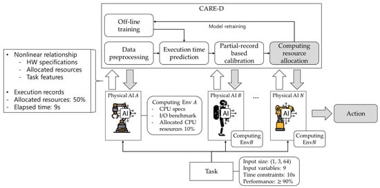
Figure 1. System overview of CARE-D in a physical AI resource management loop, where execution time predictions are used to select computing resources for physical AI tasks.

3.2. Problem Formulation

In this work, we consider execution time prediction for physical AI tasks running on heterogeneous computing platforms under dynamically changing computing resources. For each task instance, we observe the following three groups of features: hardware related features $h$, resource-level features $r$, and task-specific features $t$. Hardware features $h$ include descriptors such as CPU architecture, family, core count, memory size, operating system, and performance indices. Resource-level features r represent the current allocation state, for example, computing resource, memory limit, and input or output bandwidth. Task features $t$ describe the workload itself, such as model type, FLOPs, input and output sizes, and workload category.

We denote by y the end-to-end execution time of a physical AI task, measured from the start of model loading or simulation initialization to the completion of computation and termination under a given combination of $h$, $r$, and $t$. The execution time can then be regarded as a multivariate function

$$y=f\left(h, r, t\right),$$

(1)

where $f$ captures the joint influence of hardware, resource levels, and task characteristics on the execution time. For learning, we construct a feature vector $x$ by concatenating the three feature groups

$$x=\left[h, r, t\right],$$

(2)

and train a parametric predictor $f$ with parameters $\theta$ that maps $x$ to an estimated execution time.

$$\widehat{y}=f_{\theta }\left(x\right)$$

(3)

In this paper, $\widehat{y}$ represents the zero-history prediction of CARE-D, that is, the execution time estimate produced by the deep neural network when no execution records from the target environment are used for adaptation. In the few-history setting, we additionally assume that for a new environment $e$, a small calibration set $C_e=\left\{\right(x_i, y_i\left)\right\}$ is available with only 1 to k execution records. CARE-D then adjusts the zero-history prediction $\widehat{y}$ using these few samples through an environment-specific calibration mechanism described in the following subsections.

3.3. DNN-Based Execution Time Predictor

Based on the formulation in Section 3.2, CARE-D first learns a universal deep neural network predictor that approximates the execution time function $f$ over multiple environments. Given a feature vector $x=[h,r,t]$ and the corresponding measured execution time $y$, the predictor $f_{\theta }$ is trained to produce an accurate zero-history estimate $\widehat{y}=f_{\theta }\left(x\right)$ for unseen task and resource configurations, including those from environments that are not explicitly present in the training set.

The input to the network is a concatenation of three feature groups. The hardware feature vector $h$ contains CPU and platform descriptors such as CPU family, core count, clock frequency, memory capacity, operating system, and pre-measured performance indices for CPU, memory, and I/O. The resource-level vector $r$ represents the current allocation state, including CPU quota or percentage, memory limit, and logical I/O bandwidth. The task feature vector $t$ describes workload characteristics such as model type, FLOPs, input and output tensor sizes, and workload category. By jointly encoding these three groups in a single vector $x$, the predictor can capture interactions between hardware characteristics, resource levels, and task properties that determine the end-to-end execution time of physical AI workloads.

Categorical features such as CPU architecture, CPU model, operating system, and task type are converted into numeric representations before being fed into the network. In our implementation, these attributes are encoded as one-hot vectors and concatenated with the continuous features, while the performance indices for CPU, memory, and I/O are included as normalized scalar inputs that summarize baseline capabilities of each environment.

The predictor $f_{\theta }$ is implemented as a fully connected feed-forward neural network with several hidden layers. Each hidden layer applies an affine transformation followed by a rectified linear unit activation. Batch normalization and dropout are optionally applied after some layers to stabilize training and mitigate overfitting. The final output layer produces a single scalar that represents the predicted execution time $\widehat{y}$ for the given configuration $x$. All environments share the same network parameters $\theta$, so that a single model can learn from data collected on heterogeneous platforms and resource settings.

The parameters $\theta$ are learned by minimizing a loss function over a training set $D=\left\{\right(x_j,y_j\left)\right\}.$ To reduce the influence of extreme long-running outliers and to better capture multiplicative variations, the loss is computed on log-transformed execution times. In the simplest form, we minimize the mean absolute error in the log domain, as follows:

$${\theta }^{*}=\mathrm{a}\mathrm{r}\mathrm{g} \underset{\theta }{\min }{\displaystyle \frac{1}{\left|D\right|}}\sum _{(x_j,y_j)\in \theta }|\log \left({\widehat{y}}_j\right)-\log \left(y_j\right)|,$$

(4)

where ${\widehat{y}}_j=f_{\theta }\left(x_j\right)$. The resulting predictor $f_{{\theta }^{*}}$ provides the zero-history execution time estimate for any new configuration $x$ and serves as the base model that will be adapted by the few-history calibration mechanism described next.

3.4. Few-History Calibration Mechanism

While the universal predictor $f_{{\theta }^{*}}$ can generalize across multiple environments, there remain environment-specific effects that are difficult to capture purely from feature descriptors, such as subtle differences in operating system scheduling, firmware behavior, or background interference. CARE-D addresses these residual discrepancies through a lightweight few-history calibration mechanism that adjusts the scale of the zero-history predictions using a small number of execution records from each new environment.

For a new environment $e$, we assume that a small calibration set

$$C_e=\left\{\right(x_i, y_i\left)\right|i=\mathrm{1,2},\dots ,k\}$$

(5)

is available, where each pair $(x_i, y_i)$ corresponds to a task configuration and its measured execution time under environment $e$. For each calibration sample, the zero-history predictor produces an estimate ${\widehat{y}}_j=f_{{\theta }^{*}}\left(x_j\right)$. We then compute a per sample ratio ${\rho }_i$ between the measured and predicted execution times,

$${\rho }_i={\displaystyle \frac{y_i}{{\widehat{y}}_j}}$$

(6)

The environment-specific scaling factor ${\mathsf{\gamma }}_e$ is obtained by averaging these ratios, where the same $k$ denotes the number of calibration samples in environment $e$.

$${\mathsf{\gamma }}_e={\displaystyle \frac{1}{k}}\sum _{i=1}^k{\rho }_i.$$

(7)

When only a single calibration record is available ($k=1$), ${\mathsf{\gamma }}_e$ reduces to the simple ratio between the measured and predicted execution time for that configuration. As more calibration samples are gathered, the averaging process reduces the impact of noise in individual measurements and yields a more stable estimate of the environment-specific scaling.

Given ${\mathsf{\gamma }}_e$, CARE-D produces a calibrated execution time prediction $\tilde{y}$ for any configuration $x$ in environment $e$ by rescaling the zero-history estimate, as follows:

$$\tilde{y}={\mathsf{\gamma }}_e{f}_{{\theta }^{*}}\left(x\right).$$

(8)

Intuitively, the universal predictor $f_{{\theta }^{*}}$ learns the nonlinear shape of the execution time surface over hardware, resource, and task features, while the scalar ${\mathsf{\gamma }}_e$ compensates for systematic vertical shifts between environments that are not fully explained by the input features. In practice, our dataset shows that a small number of calibration records, often between one and five samples per environment, is sufficient to obtain a reliable scaling factor for cross-environment prediction. To avoid leakage between calibration and evaluation, calibration samples from the target environment are used only to compute ${\mathsf{\gamma }}_e$ and are excluded when computing evaluation metrics in the experimental section. The calibration procedure is summarized in Algorithm 1.

Algorithm 1 Few-History based Calibration Algorithm

Input: Trained predictor $f_{{\theta }^{*}}$;     Calibration set $C_e={\left\{\right(x_i,y_i\left)\right\}}_{i=1}^k$ in environment $e$.     Output: Calibrated prediction $\tilde{y}$ for a new input $x$ in environment $e$. 1: for each calibration sample $(x_i,y_i)$ in $C_e$ do 2:      compute the zero history prediction ${\widehat{y}}_i=f_{{\theta }^{*}}\left(x_i\right)$. 3: end 4: Compute the per sample ratios ${\rho }_i=y_i/{\widehat{y}}_i$ for $i=1,\dots ,k$. 5: Estimate the environment specific scaling factory ${\gamma }_e={\displaystyle \frac{1}{k}}{\sum }_{i=1}^k{\rho }_i$. 6: For any new configuration $x$ in environment $e$, obtain the zero history     prediction $\tilde{y}=f_{{\theta }^{*}}\left(x\right)$. 7: return the calibrated prediction $\tilde{y}={\gamma }_e\widehat{y}$.

3.5. Calibration Assumptions

The calibration mechanism in CARE-D relies on the assumption that the dominant cross-environment differences in execution time can be approximated by a multiplicative scaling factor that is relatively stable across configurations within the same environment. This does not require strict separability in the form

$$y=f\left(h,r,t\right)=f_0(h,r,t)·g_e,$$

(9)

but assumes that, after the universal predictor $f_{{\theta }^{*}}$ has captured the main nonlinear dependencies on hardware, resource levels, and task features, the remaining environment-specific bias can be modeled approximately by a single scalar multiplier ${\mathsf{\gamma }}_e$.

In practice, we observe that reducing computing resources tends to increase execution time in a mostly monotonic fashion for the classes of physical AI workloads considered in this study, although measurement noise, background load, and thermal effects may introduce deviations. The few-history calibration does not attempt to correct fine-grained non-monotonic behavior, but instead focuses on aligning the overall scale of the predicted runtime curve with the local distribution of measurements in each environment.

This simple multiplicative model has two important advantages for physical AI systems. First, it can be estimated from very few samples, making it feasible to adapt to new environments without extensive profiling. Second, it preserves the nonlinear shape learned by the DNN predictor over hardware, resource, and task features, so that the effect of changing computing resource levels remains consistent with the training data. At the same time, we acknowledge that a single scalar factor may not fully capture all environment-specific effects, especially in heterogeneous or heavily loaded systems. Extending CARE-D to more expressive calibration models that can correct non-uniform distortions of the runtime curve is left as future work.

3.6. Resource-Aware Usage in Physical AI Systems

Finally, we outline how the calibrated execution time predictions produced by CARE-D can be used for resource allocation in physical AI systems. Consider a physical AI task with hardware descriptor $h$, task features $t$, and a set of candidate resource levels $R$, for example, discrete computing resources. Given a timing constraint or deadline $D$, a simple resource selection policy is to choose the smallest resource level $r^{*}\in R$ whose calibrated execution time prediction satisfies the following deadline:

$$r^{*}=\mathrm{a}\mathrm{r}\mathrm{g} \underset{r\in R}{\min }\left\{r\right|\tilde{y}(h,r,t)\le D\},$$

(10)

where $\tilde{y}(h,r,t)$ is obtained from CARE-D using the calibrated predictor for the current environment. This discrete search can be implemented efficiently by evaluating CARE-D on the finite set of candidate resource levels. To improve robustness against prediction errors, a conservative margin can be introduced by tightening the effective deadline or by selecting a slightly higher resource level than the minimal one. For example, the scheduler may require $\tilde{y}\left(h,r,t\right)\le \alpha D$ with a safety factor $\alpha <1$, or choose the next larger computing resource above $r^{*}$. These simple policies illustrate how CARE-D can serve as an execution time oracle for existing resource managers and schedulers in physical AI systems, enabling resource-aware decisions under limited profiling and dynamically changing computing conditions.

4. Experiments and Analysis

4.1. Dataset Description

To verify the proposed CARE-D, a DNN-based execution time prediction and few-history calibration scheme for physical AI systems, we conducted experiments using execution logs collected from real industrial deployments. The dataset is explicitly designed for cross-environment execution time prediction and consists of the following two representative physical AI workloads: discrete-event manufacturing simulations and neural network inference-based production forecasting, collected under varying hardware resources.

4.1.1. Data Sources and Collection Procedure

The dataset used in this study was constructed using two commercial applications developed by Samco in South Korea, both of which are actively deployed in real production environments. The first application is an industrial process simulator designed for discrete-event manufacturing operations such as scheduling, defect generation, and resource assignment. The second application consists of AI-based prediction models that perform neural network inference for production forecasting. These two types of tasks were executed repeatedly under various CPU allocation ratios ranging from 1% to 100% and across multiple hardware configurations. During each execution, detailed logs were collected, including task-related information such as input data and task type, environment characteristics such as CPU architecture, number of cores, and threads, and memory capacity, as well as execution resource parameters such as CPU usage and performance indices. The total elapsed execution time (in seconds) was recorded as the target variable. In total, 123,930 execution records were gathered from 11 distinct computing environments, each representing a unique combination of task configuration, CPU utilization ratio, and hardware specification.

4.1.2. Feature Composition

Each data sample comprises 20 features that can be categorized into three groups. The first group, workload features, includes parameters such as CPU percentage, defect rate and volume, processing time, waiting time, work time, planned operations, quantity produced, product mappings, and resource inventory. The second group, hardware features, describes system characteristics including CPU architecture, family, model, number of cores and threads, RAM capacity, and CPU limit. The third group, performance index features, contains normalized metrics for CPU, memory, and I/O performance. The target variable, execution time, spans from 0.15 to 2847 s, with a median value of 127.3 s, thereby encompassing both lightweight neural inference tasks and long-running simulation processes.

4.1.3. Data Distribution

Each workload was executed at multiple CPU utilization levels from 1% to 100% in 1% increments, and multiple repetitions per configuration were included to capture variability. System metrics such as CPU, memory, and I/O utilization were log-normalized across environments for model input consistency.

A detailed description is shown in Table 1.

Table 1. Data distribution details.

Metric	Min	Median	Max	Mean ± Std
Samples per environment	7245	9156	11,832	9090 ± 1234
Unique workloads	42	50	58	49.5 ± 4.2
Execution time (s)	0.15	127.3	2847.5	215.6 ± 289.3
Metric	Min	Median	Max	Mean ± Std
Samples per environment	7245	9156	11,832	9090 ± 1234

4.2. Experimental Environment Configuration

4.2.1. Hardware and Operating Systems

Experiments were performed on 11 distinct hardware environments, each with different CPU generations, core/thread counts, and memory capacities to reflect diverse computing conditions of physical AI systems. Table 2 summarizes the configuration details of each environment. The CPU generations are Intel 10th, 13th, and 14th (from Comet Lake to Raptor Lake Refresh). Memory capacities are from 31.7 to 63.9 GB, while operating systems consist of 9 Windows 11 and 2 Ubuntu 22.04. This diversity ensures that the proposed method is tested under cross-generation, cross-memory, and cross-OS conditions, capturing realistic variability in edge or embedded physical AI deployments.

Table 2. Environment description.

Environment	CPU Model	Architecture	Cores/Threads	RAM (GB)	OS
E1	Intel i7-13700K (Model 167)	Intel64	8/16	63.8	Windows 11
E2	Intel i9-10900K (Model 165)	Intel64	10/20	31.9	Windows 11
E3	Intel i9-14900K (Model 183)	Intel64	20/28	31.7	Windows 11
E4	Intel i7-14700K (Model 183)	Intel64	16/24	63.8	Windows 11
E5	Intel i7-13700K (Model 167)	Intel64	8/16	63.8	Windows 11
E6	Intel i7-13700K (Model 167)	Intel64	16/24	62.6	Ubuntu 22.04
E7	Intel i9-10900K (Model 165)	Intel64	10/20	63.9	Windows 11
E8	Intel i7-14700K (Model 183)	Intel64	16/24	63.8	Windows 11
E9	Intel i7-13700K (Model 167)	Intel64	8/16	31.8	Windows 11
E10	Intel i9-10900K (Model 165)	Intel64	10/20	63.9	Windows 11
E11	Intel i7-13700K (Model 167)	Intel64	16/24	62.6	Ubuntu 22.04

4.2.2. Model Training and Validation Procedure

To evaluate how the proposed method can generalize across heterogeneous computing environments, we adopted a leave-one-environment-out (LOEO) validation procedure. In each round of evaluation, one environment was excluded from training and used exclusively for testing, while the remaining environments were used for model learning. This process was repeated until every environment had served once as the unseen test case, and the final performance was obtained by averaging the results over all folds.

This approach offers two key advantages. First, it provides a rigorous measure of cross-environment generalization, as the model is evaluated on hardware configurations it has never encountered during training. Second, it prevents environment-specific overfitting, which often occurs when a model learns hidden correlations unique to particular systems or datasets. By averaging the results from all folds, we obtained a fair and stable assessment of prediction accuracy and adaptability.

For calibration-based experiments in the few-history setting, we assume that only a small number of execution records is available from the target environment. In each LOEO fold, the records in the held-out environment are further split into a small calibration subset and a disjoint test subset, so that no configuration appears in both calibration and evaluation. A small number of measured execution times, typically between one and five samples from the calibration subset, is used to compute environment-specific scaling factors for CARE-D without retraining the DNN models. Calibration samples are used solely for estimating these scaling factors and are excluded from all evaluation metrics, preventing leakage between calibration and test data.

4.3. Experimental Setup and Evaluation Metrics

The collected dataset of 123,930 execution records from 11 heterogeneous computing environments was used for all experiments. Within each LOEO fold, records from the ten training environments were split into a training subset (80%) and a validation subset (20%), while all records from the held-out environment were used exclusively as the test set. The training subset was used to optimize the parameters of the proposed DNN-based execution time prediction model, and the validation subset guided early stopping and learning-rate adjustment. The test subset provided an unbiased estimate of generalization performance under unseen hardware and operating system configurations.

All experiments were conducted on the 11 hardware environments summarized in Table 3. For each environment, the model was trained and evaluated on a mixture of AI-based production-forecasting workloads and discrete-event simulation tasks, with CPU utilization levels varied from 1% to 100% in 1% increments. The training process used the Adam optimizer with a learning rate of 0.001 and Mean Squared Error (MSE) as the loss function, with early stopping based on validation loss convergence. Continuous feature values, including FLOPs, input/output size, and CPU percentage, were log-transformed or log-normalized before training to mitigate scale imbalance and improve numerical stability.

Table 3. The comparison models for the execution time prediction.

Model	Type/Library	Key Characteristics
Linear Regression (LR)	Linear/scikit-learn	Learns a direct proportional relationship between resource features (e.g., CPU%) and execution time; useful as a baseline for simple linear dependencies
Ridge Regression	Linear (L2 regularized)/scikit-learn	Captures linear correlations between environment and task features while reducing sensitivity to multicollinearity through L2 regularization
Lasso Regression	Linear (L1 regularized)/scikit-learn	Performs feature selection by identifying the most influential environmental or workload factors affecting execution time
Decision Tree Regressor	Nonlinear/scikit-learn	Learns hierarchical decision rules that map combinations of hardware and workload features to distinct execution-time ranges
Random Forest Regressor	Ensemble of trees/scikit-learn	Aggregates multiple decision trees to capture diverse feature–time relationships, improving robustness against noise and overfitting
Gradient Boosting Regressor (GBR)	Ensemble boosting/scikit-learn	Sequentially minimizes prediction errors by refining weak learners, effectively modeling nonlinear dependencies between environment parameters and runtime
XGBoost Regressor	Gradient boosting (optimized)/XGBoost 1.5.0	Employs regularized boosting to efficiently learn complex feature interactions across heterogeneous computing environments
Proposed DNN Regressor	Deep neural network/PyTorch 1.9.0	Learns high-dimensional nonlinear mappings between hardware–task feature combinations and execution time, achieving adaptability across unseen environments
Graph Neural Network (GNN)	Graph-based deep learning/PyTorch Geometric, DGL	Learns execution-time patterns by modeling relational dependencies among hardware and task features as graph structures.
Long Short-Term Memory (LSTM)	Recurrent neural network/PyTorch, TensorFlow 2.8.0	Captures temporal or sequential dependencies in workload patterns that influence execution time.
Support Vector Regression (SVR)	Kernel-based regression/scikit-learn	Uses kernel functions to model nonlinear relationships between environment parameters and runtime with strong performance on small datasets.
Transformer-Based Regressor	Attention-based deep learning/PyTorch	Learns global feature interactions through self-attention, effectively modeling complex execution-time dependencies.

To verify the adaptability of the proposed few-history based calibration method, additional evaluations were performed by applying calibration using k = 1, 5, 10, 15, and 20 measured execution times from the calibration subset of the target environment in each LOEO fold. After estimating environment-specific scaling factors from these k samples, the model predicted execution times for the remaining configurations in the disjoint test subset. This procedure validates the ability of CARE-D to maintain a high prediction accuracy when only a small number of runtime measurements can be collected in a new physical AI environment.

The evaluation primarily employed the following two key metrics: Mean Absolute Error (MAE) and Accuracy. MAE quantifies the absolute deviation between predicted and actual execution times, averaged over all test samples. The accuracy metric measures the proportion of predictions whose relative error falls within a 10% threshold, providing an interpretable view of how often the model meets a practical timing margin for latency-sensitive physical AI tasks. These metrics were computed both before and after few-history calibration to assess the improvement in predictive accuracy and adaptability across the various environments.

To clearly evaluate the adaptability of the proposed model, the following two experimental settings were defined: zero-history and few-history based calibration. In the zero-history setting, the DNN predictor and baseline models were evaluated on the held-out environment without any calibration data, representing the baseline cross-environment generalization performance. In the few-history setting, each model was additionally provided with a small number of actual runtime samples (typically 1–5 in the main analysis) from the target environment to perform calibration before predicting the remaining configurations. The calibrated predictions were then compared with the zero-history outputs of CARE-D and with conventional regression-based models under the same LOEO folds, allowing a quantitative assessment of how much the few-history calibration mechanism improves execution time prediction accuracy and stability relative to the uncalibrated case.

4.4. Comparison Models

To validate the performance of the proposed CARE-D, we compared it against a wide range of baseline models under identical experimental settings. The comparison covers three families of methods, as follows: classical regression models, general-purpose deep learning models, and the proposed CARE-D architectures implemented as fully connected DNNs. All models receive the same 20-dimensional feature vector described in Section 4.1 and are trained and evaluated using the LOEO protocol and calibration settings defined in Section 4.2 and Section 4.3.

Table 3 summarizes the baseline models used for execution time prediction. The regression family includes linear models such as Linear Regression, Ridge, Lasso, and ElasticNet, which capture simple linear correlations between environment and workload features and provide a reference performance for linearly separable relationships. Tree-based ensemble methods such as Decision Tree, Random Forest, Gradient Boosting, and XGBoost are included to model nonlinear interactions between hardware, resource, and workload features through hierarchical decision rules and boosted ensembles. Support Vector Regression is also considered to investigate kernel-based nonlinear regression on the same feature space. These models are widely used in performance prediction and scheduling research and serve as baselines for heterogeneous computing environments.

The deep learning baselines comprise a generic graph neural network, an LSTM network, and a Transformer-based regressor, which represent typical neural architectures for graph-structured, sequential, and attention-based modeling. The graph neural network aims to capture relational dependencies among hardware and task features by treating them as graph nodes. The LSTM models potential sequential or temporal patterns in workload behavior. The Transformer-based regressor leverages self-attention to learn global feature interactions. These models help assess whether more complex inductive biases used in other domains are suitable for execution time prediction under heterogeneous physical AI environments.

CARE-D itself is implemented as a family of fully connected feed-forward DNN architectures that share the same input and output interfaces but differ in depth and width. Five variants were developed to balance model capacity and computational efficiency. All variants take as input the concatenated feature vector x, including hardware descriptors, resource-level features, and task-specific features, and produce a scalar execution time prediction. Their configurations are summarized conceptually in Table 4.

Table 4. The details of the CARE-D models.

Model	Architecture	Hidden Layers	Regularization	Purpose
${CARE-D}_{small}$	Small	2 (64, 32)	Dropout (0.1), BatchNorm	Lightweight baseline for fast inference
${CARE-D}_{medium}$	Medium	3 (128, 64, 32)	Dropout (0.1), BatchNorm	Relatively balanced accuracy
${CARE-D}_{large}$	Large	4 (256, 128, 64, 32)	Dropout (0.1), BatchNorm	Captures higher nonlinear interactions
${CARE-D}_{x\_large}$	Extra large	5 (512, 256, 128, 64, 32)	Dropout (0.1), BatchNorm	High-capacity model for complex nonlinearity
${CARE-D}_{deep}$	Deep variant	6+ layers (1024 to 32)	Dropout (0.1), BatchNorm	Investigates the hidden nonlinear relationships between features

All CARE-D variants use rectified linear unit activations in hidden layers and optionally apply batch normalization and dropout to mitigate overfitting. A single set of network parameters is shared across all environments so that the model learns a unified mapping from feature space to execution time and provides zero-history predictions for unseen configurations. Few-history calibration is then applied on top of these DNN predictors in the experimental analysis of Section 4.5. In the detailed result discussion, we primarily focus on the small, medium, and large CARE-D configurations, since the extra-large and deep variants showed unstable cross-environment behavior and a tendency for overfitting, providing limited additional benefit over the more compact architectures.

4.5. Experimental Results and Analysis

The experiments compared zero-history and few-history scenarios to evaluate how calibration affects prediction accuracy and mean absolute error (MAE) across diverse computing environments. All models were evaluated using 11-fold LOEO validation so that each hardware configuration served once as an unseen target environment.

The results show that DNN models exhibited some performance gains from few-history-based calibration, while regression models showed minimal or even negative change. Across all DNN architectures, the average accuracy increased from 29.4% to 36.7%, and the MAE dropped from 574.3 s to 32.3 s. In contrast, regression models showed only a 0.4% change in accuracy and a slight MAE increase of 1.9 s, indicating that calibration has negligible benefit for static regression models.

The comparative experiments were conducted under two distinct settings to evaluate the adaptability of the prediction models. The first is the zero-history setting, where the model directly predicts the execution time in unseen environments without any runtime history or calibration. The second is the few-history-based calibration setting, where one or a few measured execution time samples from the target environment are used to perform lightweight calibration before predicting the remaining processes in that environment.

Both settings were tested using the following three DNN architectures: DNN (64, 32), DNN (128, 64, 32), and DNN (256, 128, 64). Other, deeper DNN models were not included in the comparison because excessively large models tend to capture noise rather than meaningful patterns in the training data, which can lead to overfitting when the true relationship between features is relatively simple. This may indicate that the applications used in this paper contain an approximately monotonic relationship between task and environment features and execution times. The detailed experimental results and analysis are described in the following subsections.

4.5.1. Comparison in Zero-History Environments

Figure 2 and Figure 3 summarize how the three CARE-D architectures behave in zero-history and few-history conditions. In the zero-history setting (k = 0), shown in Figure 2, the models must predict execution time in previously unseen hardware–software environments without any calibration samples. Under this challenging condition, CARE-D achieves an accuracy between approximately 28% and 36% within the 10% relative error band, and the performance varies noticeably with architectural capacity.

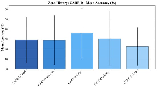
Figure 2. The performance of the CARE-D models without the calibration.

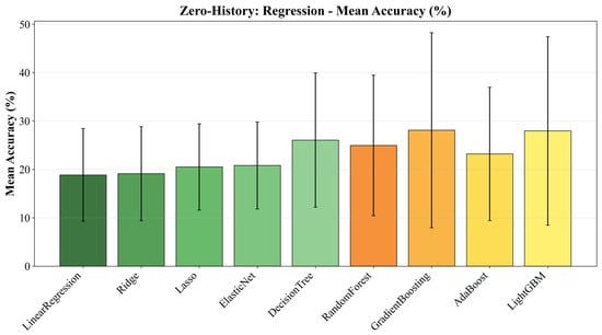
Figure 3. The overall performances of regression models.

The large CARE-D (256–128–64) provides the best-performing zero-history baseline. Its higher capacity allows the network to better capture nonlinear interactions between workload features and environment characteristics, yielding the highest accuracy among the three plotted architectures. In contrast, the small CARE-D (64–32) shows a clearly lower accuracy, which reflects its limited representation capacity and reduced ability to generalize across diverse workloads and environments. The medium CARE-D (128–64–32) lies between these two extremes and offers a balanced trade-off between expressiveness and stability. These observations indicate that, before calibration, zero-history performance is primarily governed by the depth and width of the architecture.

Figure 3 further compares the zero-history and few-history performance of the same architectures across all 11 environments. For CARE-D (64–32), few-history calibration produces the largest relative gain, with an average accuracy increase of about 9.93 percentage points over its zero-history baseline. The medium CARE-D (128–64–32) also exhibits some improvements of roughly 8.98 percentage points. These results show that compact architectures, which underfit slightly in zero-history, can be effectively “completed” by a small number of environment-specific calibration samples, achieving a cross-environment performance with only limited profiling.

By contrast, the large CARE-D (256–128–64) already provides a zero-history baseline, so its additional gain from calibration is smaller but consistently positive. In this case, calibration mainly refines the prediction surface by reducing mean absolute error and correcting residual environment-specific bias rather than increasing accuracy. This behavior is consistent with the interpretation that most cross-environment variability can be expressed as a smooth scaling of the DNN’s predicted runtime curve, which the multiplicative calibration factor is designed to correct.

We also evaluated a deeper CARE-D variant (256–256–64–32), which is omitted from Figure 2 and Figure 3 because of its unstable zero-history behavior and low overall accuracy. This over-parameterized model tended to overfit environment-specific noise rather than capturing the underlying monotonic relationship between features and execution time, and it only became usable after calibration reduced its MAE. This observation suggests that simply increasing depth and width does not guarantee better cross-environment generalization.

Overall, the combined results from Figure 2 and Figure 3 justify selecting CARE-D (128–64–32) as the representative architecture in the subsequent analysis. It offers a reasonable zero-history accuracy, a large and consistent few-history gain comparable to the small architecture, and a lower risk of instability than deeper variants while keeping computational cost manageable for practical physical AI deployments.

Figure 4 also reports the zero-history performance of general-purpose deep learning models that do not explicitly encode the structure of execution-time prediction. The LSTM reaches around 25% accuracy, whereas the GNN drops to roughly 6% and the Transformer remains near 2–3%, which is effectively comparable to random prediction. These results indicate that the inductive biases of sequence-based (LSTM), graph-based (GNN), and attention-based (Transformer) architectures are fundamentally misaligned with the characteristics of execution-time prediction in this setting: their internal mechanisms do not naturally account for the coarse, environment-level scaling effects that dominate this task, leading to poor zero-history generalization.

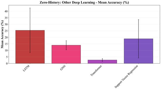
Figure 4. The performance comparison of the deep learning models in the other DL category.

4.5.2. Comparison in Few-History Environments

In the few-history setting, the models are allowed to use only a small number of execution records from the target environment to adjust their predictions before being evaluated on the remaining configurations. This setting reflects realistic physical AI deployments in which extensive profiling is not feasible and only a handful of measurements can be collected when a new controller or plant is introduced.

Figure 5 shows how CARE-D responds to few-history calibration for different values of $k$. When only 1–5 calibration samples are available from the target environment, CARE-D models exhibit a consistent improvement over their zero-history baselines. Across the three main architectures, the average accuracy increases from 29.4% to 36.7%, while MAE decreases from 574.3 s to 32.3 s after calibration. The small CARE-D (64–32) and the medium CARE-D (128–64–32) obtain the largest few-history gains, with accuracy improvements of approximately +9.93 and +8.98 percentage points, respectively, compared to their zero-history performance. These results indicate that CARE-D can rapidly estimate and compensate for broad environment-specific scaling differences when given only a few samples from the target environment. However, as $k$ grows beyond about 5–10, the additional benefit diminishes, and in some cases, accuracy begins to decline, suggesting overfitting to the limited calibration subset rather than generalization to all workloads in the environment.

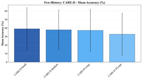
Figure 5. The overall performance comparison of CARE-D with the calibration. The deep CARE-D was omitted for low accuracy.

Figure 6 summarizes the behavior of classical regression models, including linear, tree-based, and kernel-based regressors, when few-history calibration is applied. In contrast to CARE-D, these models show almost no meaningful accuracy gain: the observed changes remain within a very narrow band of roughly 0.01–0.02 percentage points across different values of $k$, and in some environments, the calibrated models even exhibit a slightly worse accuracy than their zero-history baselines. A closer inspection of the top-performing regressors (Gradient Boosting, Random Forest, XGBoost, SVR, and LightGBM) confirms this trend. Small positive changes occasionally appear, but they are rare and typically accompanied by degradation in MAE or $R^2$, so the overall fit to the runtime distribution does not improve.

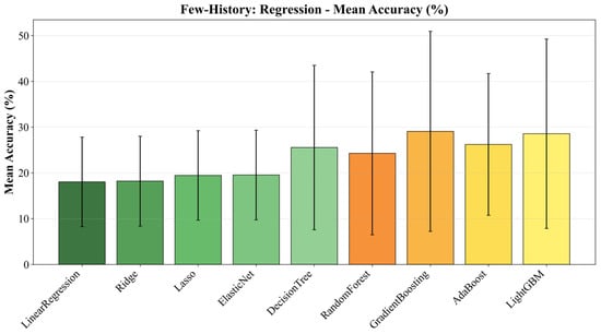
Figure 6. The accuracy comparison of the traditional regression models.

This limited effect is consistent with the inductive bias of regression models. Tree-based ensembles and SVR already encode a piecewise-constant or locally linear approximation of the feature–runtime mapping based on the training environments, so their zero-history predictions are dominated by feature-level relational patterns rather than by a single global scale factor. As a result, multiplying predictions by an environment-specific ratio estimated from a few samples has little impact on the underlying error structure and can even push the predictions away from the true values. In other words, the simple ratio-based calibration that is effective for CARE-D provides little benefit for these static regression models, even though the same calibration mechanism and few-history budget are applied.

Other deep learning models show a very different few-history behavior from CARE-D. Figure 7 reports the performance of LSTM, GNN, and Transformer when the same ratio-based calibration is applied. LSTM shows a small improvement when $k=1$, but its accuracy quickly saturates and even decreases as more calibration samples are added, indicating that additional few-history information does not translate into better generalization. GNN begins to deteriorate almost immediately, with accuracy dropping below its zero-history level even for small $k$, and Transformer remains close to its very low zero-history accuracy (around 2–3%) across all values of $k$, effectively failing to exploit the calibration samples at all.

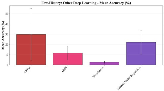
Figure 7. The overall performance of the other category’s deep learning models.

These trends suggest that the internal representations of LSTM, GNN, and Transformer in this setting do not interact well with a simple global scaling factor. Their complex nonlinear transformations are not aligned with the dominant cross-environment effect in our dataset, so injecting a handful of environment-specific samples tends to amplify existing prediction errors rather than correct them. As a result, few-history calibration does not provide a consistent gain for these models, in sharp contrast to CARE-D, which was explicitly designed to be amenable to such ratio-based adjustment.

4.5.3. Zero-History vs. Few-History

Figure 8 shows the average performance of the three model families—CARE-D, classical regression models, and other deep learning baselines—under zero-history and few-history conditions. In the zero-history setting, as shown in Figure 8a, CARE-D already provides the best-performing cross-environment generalization among all evaluated methods. Its average accuracy is several percentage points higher than the best ensemble regression models, consistent with the overall result that CARE-D achieves a baseline accuracy about 6.06 percentage points higher than the best regression baseline. Regression models form a stable but lower-performing group, while the other deep learning models (LSTM, GNN, and Transformer) remain clearly below CARE-D, and in some cases, close to random prediction, reflecting their misaligned inductive biases for execution-time prediction.

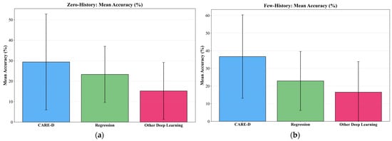
Figure 8. The average performance comparison among the models in the three categories in zero-history and few-history conditions: (a) the performance comparison in zero-history environments and (b) the comparison in few-history environments.

When few-history calibration is applied (Figure 8b), the difference between model families becomes even more pronounced. On average, CARE-D improves from 29.4% to 36.7% accuracy and its MAE drops from 574.3 s to 32.3 s, indicating that a small number of environment-specific samples is sufficient to refine its predictions. Regression models, in contrast, show almost no change: their average accuracy varies by only about −0.4 percentage points and MAE increases slightly by 1.9 s, confirming that ratio-based calibration has negligible benefit for these static predictors. The other deep learning models exhibit unstable behavior, with LSTM showing only marginal and inconsistent gains, while GNN and Transformer often degrade relative to their already low zero-history performance.

Overall, Figure 8 highlights that few-history information is model-dependent in this setting. CARE-D is the only family that consistently converts 1–5 calibration samples into accuracy and MAE improvements, whereas regression and other deep learning models remain largely unchanged or even deteriorate. This pattern supports the claim that CARE-D is specifically well-suited for few-shot adaptation in heterogeneous physical AI environments, while conventional regressors and generic deep architectures cannot effectively exploit the same limited calibration budget.

4.5.4. Minimum Effective Sample Ratio (MESR)

To compare how efficiently each model family can exploit a few calibration samples, we analyze the Minimum Effective Sample Ratio (MESR) using the results in Figure 9. Intuitively, MESR captures how many calibration samples are required until a model reaches (or is very close to) its best few-history performance. A lower MESR, therefore, indicates that the model can make good use of very limited information from a new environment, which is critical in practical physical AI deployments where extensive profiling is not feasible.

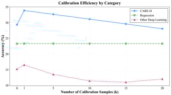
Figure 9. MESR calibration efficiency comparison among the proposal, the regression models, and the other types of deep learning models.

For CARE-D, the MESR analysis shows that a single calibration sample is typically sufficient. Across the evaluated environments, $k=1$ already yields most of the accuracy and MAE improvements observed over the entire range $k\in \{\mathrm{1,5},\mathrm{10,15,20}\}$. Combined with the results in Figure 5 and Figure 8, this means that CARE-D can obtain an average accuracy gain of about 7.29 percentage points (from 29.4% to 36.7%) and reduce MAE from 574.3 s to 32.3 s with only one or a few measurements per environment, while additional samples beyond five often provide diminishing or even negative returns. In other words, CARE-D achieves a very low MESR, indicating that its calibration mechanism is sample-efficient for cross-environment execution-time prediction.

By contrast, the regression baselines and other deep learning models exhibit poor MESR characteristics. As shown in Figure 6 and Figure 7, their accuracy curves remain almost flat or even degrade as $k$ increases, and the MAE or ${\mathrm{R}}^2$ metrics often worsen after calibration. Since these models show negligible few-history gain across all tested values of $k$, they effectively do not have a meaningful “minimum effective” sample point: increasing the number of calibration samples does not translate into performance improvement. From an MESR perspective, this implies that the cost of collecting additional measurements in a new environment is not justified for these models.

Overall, the MESR comparison in Figure 9 reinforces the earlier findings: CARE-D is not only more accurate than baseline models, but also much more sample-efficient in adapting to unseen environments. A single execution record per environment is generally enough to obtain most of the benefit of calibration, whereas regression baselines and generic deep learning architectures cannot convert additional samples into reliable gains. This property makes CARE-D particularly attractive for real-world physical AI systems, where minimizing profiling overhead is as important as maximizing prediction accuracy.

5. Conclusions

In this paper, we addressed the problem of resource-aware execution time prediction for physical AI tasks operating under heterogeneous hardware, dynamically allocated computing resources, and limited execution history. We formulated execution time as a multivariate function of hardware features, resource levels, and workload characteristics and proposed CARE-D (Calibration-Assisted Resource-aware Execution-time prediction), a universal deep neural network predictor combined with a lightweight few-history calibration mechanism. CARE-D learns a cross-environment prediction surface from 123,930 execution records collected across 11 real industrial environments, and then adapts to previously unseen environments using only a small number of measured execution times from each new target.

The experimental results demonstrated that CARE-D provides zero-history generalization and highly efficient few-shot adaptability. In the zero-history setting, CARE-D outperformed the best performing ensemble regression baseline by approximately 6.06 percentage points in accuracy within the 10% relative error band. With few-history calibration, CARE-D achieved an average accuracy gain of about 7.29 percentage points (from 29.4% to 36.7%) while reducing MAE from 574.3 s to 32.3 s, using only one to five calibration samples per environment. Architecture-level analysis showed that the medium CARE-D configuration (128–64–32) provides a favorable balance between capacity and stability, and the Minimum Effective Sample Ratio (MESR) analysis revealed that a single calibration sample ($k=1$) is typically sufficient to obtain most of the benefit, with gains up to 9.93 percentage points over its own zero-history baseline. In contrast, classical regression models and other deep learning baselines (LSTM, GNN, and Transformer) exhibit negligible or even negative few-history gains, indicating that the simple ratio-based calibration is particularly well matched to CARE-D’s DNN predictor but not to static regressors or generic neural architectures.

These properties make CARE-D a practical building block for resource-aware scheduling and runtime planning in physical AI systems, enabling deadline-aware CPU quota selection, admission control, and energy-aware allocation without extensive environment-specific profiling. At the same time, this work has limitations that open several directions for future research, as follows: extending the simple multiplicative calibration to slightly more expressive but still data-efficient forms, validating CARE-D on a broader range of platforms such as embedded CPUs, ARM-based edge devices, GPUs, and virtualized cloud instances, and integrating CARE-D with online schedulers or learning-based controllers to exploit uncertainty-aware and worst-case execution time predictions in real-time decision making.

References

- Dewi, R.S.; Kawakib, A.N.; Laili, M.N.; Fauziah, A.L.; Sabrina, S.R.; Hana, R.L. A Systematic Review of Physical Artificial Intelligence (Physical AI): Concepts, Applications, Challenges, and Future Directions. J. Artif. Intell. Eng. Appl. 2025, 4, 2246–2253. [Google Scholar] [CrossRef]
- Shaw, R.J.; Chen, B. Physical artificial intelligence in nursing: Robotics. Nurs. Outlook 2025, 73, 102495. [Google Scholar] [CrossRef] [PubMed]
- Bousetouane, F. Physical AI Agents: Integrating Cognitive Intelligence with Real-World Action. arXiv 2025, arXiv:2501.08944. [Google Scholar] [CrossRef]
- Zhou, Z.; Ning, X.; Hong, K.; Fu, T.; Xu, J.; Li, S.; Lou, Y.; Wang, L.; Yuan, Z.; Li, X.; et al. A survey on efficient inference for large language models. arXiv 2024, arXiv:2404.14294. [Google Scholar] [CrossRef]
- Garcia-Perez, A.; Miñón, R.; Torre-Bastida, A.I.; Zulueta-Guerrero, E. Analysing edge computing devices for the deployment of embedded AI. Sensors 2023, 23, 9495. [Google Scholar] [CrossRef] [PubMed]
- Heo, D.H.; Park, S.H.; Kang, S.J. Resource-constrained edge-based deep learning for real-time person-identification using foot-pad. Eng. Appl. Artif. Intell. 2024, 138, 109290. [Google Scholar] [CrossRef]
- Lema, D.G.; Usamentiaga, R.; García, D.F. Quantitative comparison and performance evaluation of deep learning-based object detection models on edge computing devices. Integration 2024, 95, 102127. [Google Scholar] [CrossRef]
- Kong, G.; Hong, Y.G. Inference latency prediction approaches using statistical information for object detection in edge computing. Appl. Sci. 2023, 13, 9222. [Google Scholar] [CrossRef]
- Li, Z.; Paolieri, M.; Golubchik, L. Inference latency prediction for CNNs on heterogeneous mobile devices and ML frameworks. Perform. Eval. 2024, 165, 102429. [Google Scholar] [CrossRef]
- Kokhazadeh, M.; Keramidas, G.; Kelefouras, V.; Stamoulis, I. Denseflex: A Low Rank Factorization Methodology for Adaptable Dense Layers in DNNs. In Proceedings of the 21st ACM International Conference on Computing Frontiers, Ischia, Italy, 7–9 May 2024; pp. 21–31. [Google Scholar] [CrossRef]
- Li, H.; Wang, Z.; Yue, X.; Wang, W.; Tomiyama, H.; Meng, L. An architecture-level analysis on deep learning models for low-impact computations. Artif. Intell. Rev. 2023, 56, 1971–2010. [Google Scholar] [CrossRef]
- Wu, J.; Wang, H.; Qian, K.; Feng, E. Optimizing latency-sensitive AI applications through edge-cloud collaboration. J. Adv. Comput. Syst. 2023, 3, 19–33. [Google Scholar] [CrossRef]
- Song, C.; Ye, C.; Sim, Y.; Jeong, D.S. Hardware for deep learning acceleration. Adv. Intell. Syst. 2024, 6, 2300762. [Google Scholar] [CrossRef]
- Duc, T.L.; Nguyen, C.; Östberg, P.O. Workload Prediction for Proactive Resource Allocation in Large-Scale Cloud-Edge Applications. Electronics 2025, 14, 3333. [Google Scholar] [CrossRef]
- Kirchoff, D.F.; Meyer, V.; Calheiros, R.N.; De Rose, C.A. Evaluating machine learning prediction techniques and their impact on proactive resource provisioning for cloud environments. J. Supercomput. 2024, 80, 21920. [Google Scholar] [CrossRef]
- Arnström, D.; Broman, D.; Axehill, D. Exact worst-case execution-time analysis for implicit model predictive control. IEEE Trans. Autom. Control 2024, 69, 7190–7196. [Google Scholar] [CrossRef]
- Bai, X.; Zhou, J.; Wang, Z. HPC Cluster Task Prediction Based on Multimodal Temporal Networks with Hierarchical Attention Mechanism. Computers 2025, 14, 335. [Google Scholar] [CrossRef]
- Amaris, M.; Camargo, R.; Cordeiro, D.; Goldman, A.; Trystram, D. Evaluating execution time predictions on GPU kernels using an analytical model and machine learning techniques. J. Parallel Distrib. Comput. 2023, 171, 66–78. [Google Scholar] [CrossRef]
- Kumar, V.; Ranjbar, B.; Kumar, A. Utilizing machine learning techniques for worst-case execution time estimation on GPU architectures. IEEE Access 2024, 12, 41464–41478. [Google Scholar] [CrossRef]
- Algarni, A.; Shah, I.; Jehangiri, A.I.; Ala’Anzy, M.A.; Ahmad, Z. Predictive energy management for Docker containers in cloud computing: A time series analysis approach. IEEE Access 2024, 12, 52524–52538. [Google Scholar] [CrossRef]
- Zhang, L.; Xie, Y.; Jin, M.; Zhou, P.; Xu, G.; Wu, Y.; Feng, D.; Long, D. A novel hybrid model for docker container workload prediction. IEEE Trans. Netw. Serv. Manag. 2023, 20, 2726–2743. [Google Scholar] [CrossRef]
- De Smedt, J.; Yeshchenko, A.; Polyvyanyy, A.; De Weerdt, J.; Mendling, J. Process model forecasting and change exploration using time series analysis of event sequence data. Data Knowl. Eng. 2023, 145, 102145. [Google Scholar] [CrossRef]
- Zou, M.; Zeng, Q.; Liu, C.; Cao, R.; Chen, S.; Zhao, Z. Prediction of Remaining Execution Time of Business Processes with Multiperson Collaboration in Assembly Line Production. IEEE Trans. Comput. Soc. Syst. 2024, 12, 1279–1295. [Google Scholar] [CrossRef]
Disclaimer/Publisher’s Note: The statements, opinions and data contained in all publications are solely those of the individual author(s) and contributor(s) and not of MDPI and/or the editor(s). MDPI and/or the editor(s) disclaim responsibility for any injury to people or property resulting from any ideas, methods, instructions or products referred to in the content. |
© 2025 by the authors. Licensee MDPI, Basel, Switzerland. This article is an open access article distributed under the terms and conditions of the Creative Commons Attribution (CC BY) license (https://creativecommons.org/licenses/by/4.0/).