Figure 1.
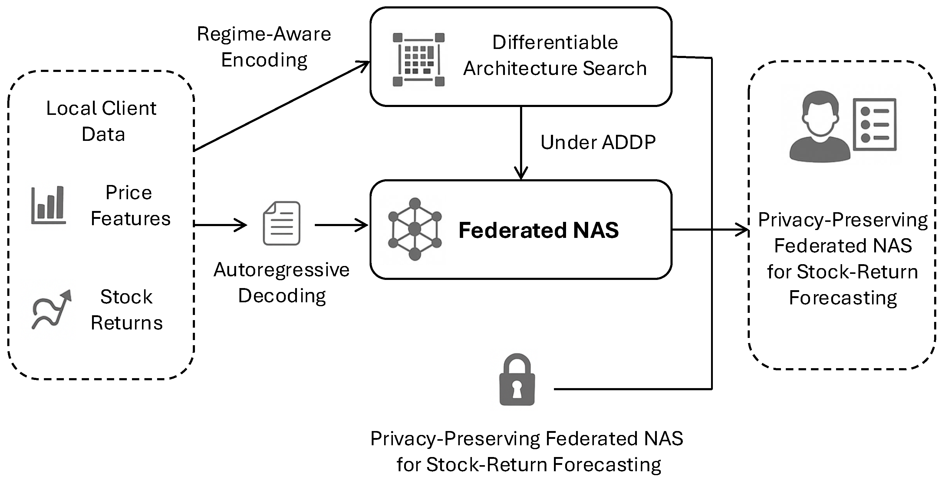
Overview of FedRegNAS. Sensitive client-side financial time-series data (price features, returns, context) are processed locally, fed into a regime-aware differentiable architecture search under ADDP, aggregated via KL-barycentric federated NAS, and deployed as a privacy-preserving stock-return forecasting model.
Figure 2.
Chronological data splits per benchmark with non-overlapping labels. Light gray: train; medium gray: validation (final 10% of training horizon); dark gray: test (calendar year 2025). Labels are positioned above (Daily-US, Minute-US) or below (Daily-Global) the bars to prevent overlap. No legend is drawn; the caption encodes color semantics.
Figure 3.
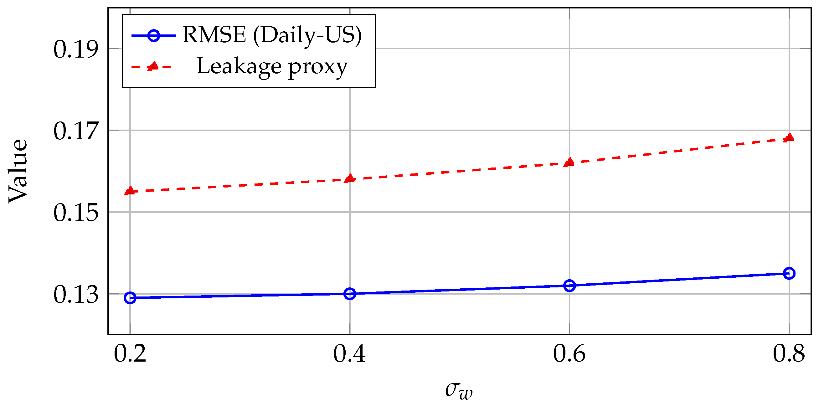
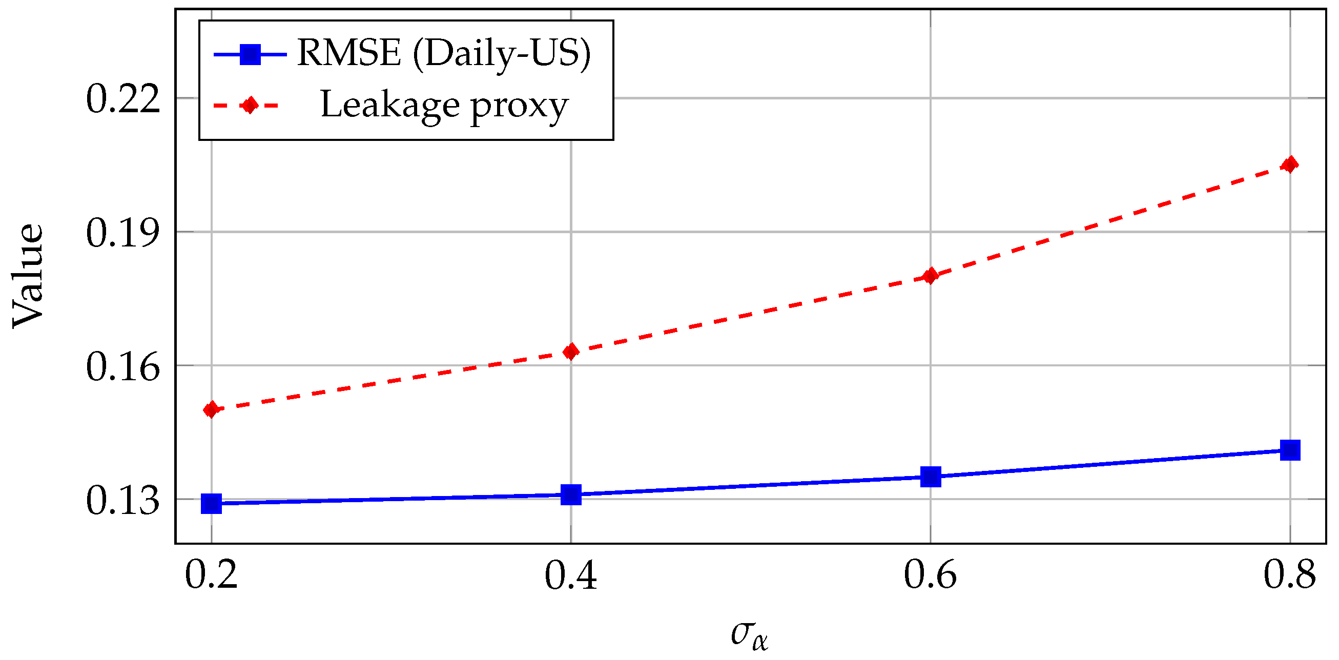
Sensitivity of FedRegNAS to decoupled DP noise scales on Daily-US. RMSE increases mainly as grows, while the effect of is comparatively mild for a fixed , indicating that architecture gradients are the dominant leakage–performance bottleneck.
Figure 3.
Sensitivity of FedRegNAS to decoupled DP noise scales on Daily-US. RMSE increases mainly as grows, while the effect of is comparatively mild for a fixed , indicating that architecture gradients are the dominant leakage–performance bottleneck.
Figure 4.
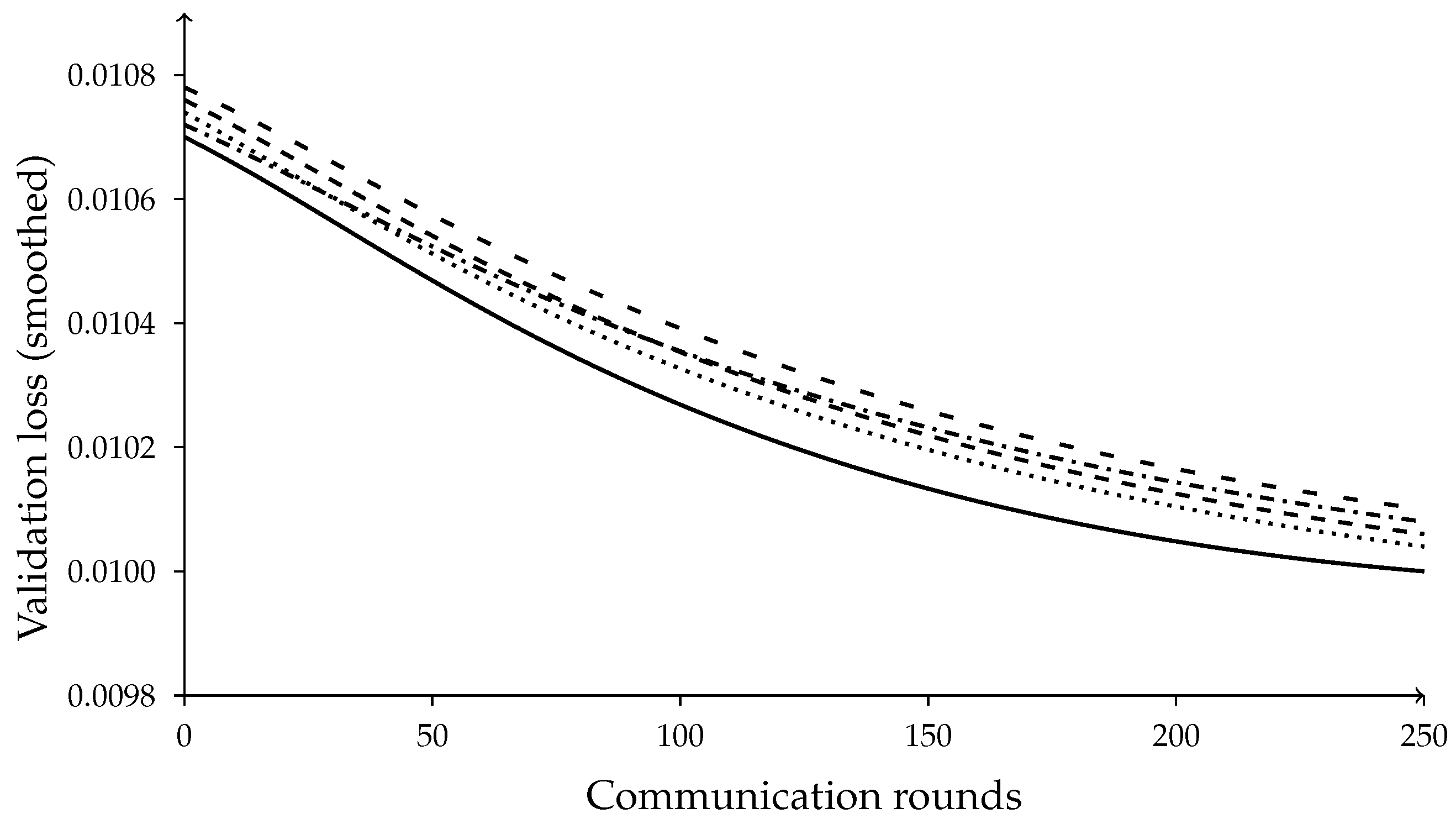
Validation-loss convergence on Daily-US. Solid: FedRegNAS; dashed/dotted variants correspond to individual ablations (mapping described in the text). The full model converges faster and to a lower final loss, showing improved stability from regime gating, KL aggregation, and trust weighting.
Figure 5.
Trust-weight entropy over rounds (lower is better). Solid: FedRegNAS; other curves correspond to ablations (mapping described in the text). The full model shows faster entropy decay, implying more decisive and stable aggregation.
Figure 5.
Trust-weight entropy over rounds (lower is better). Solid: FedRegNAS; other curves correspond to ablations (mapping described in the text). The full model shows faster entropy decay, implying more decisive and stable aggregation.
Figure 6.
Mean client uplink per round on Daily-US. Bar fills denote methods (light to dark): FedAvg-LSTM, FedProx-Trans, Centralized-DARTS, and FedRegNAS. No legend is drawn; mapping is provided here.
Figure 6.
Mean client uplink per round on Daily-US. Bar fills denote methods (light to dark): FedAvg-LSTM, FedProx-Trans, Centralized-DARTS, and FedRegNAS. No legend is drawn; mapping is provided here.
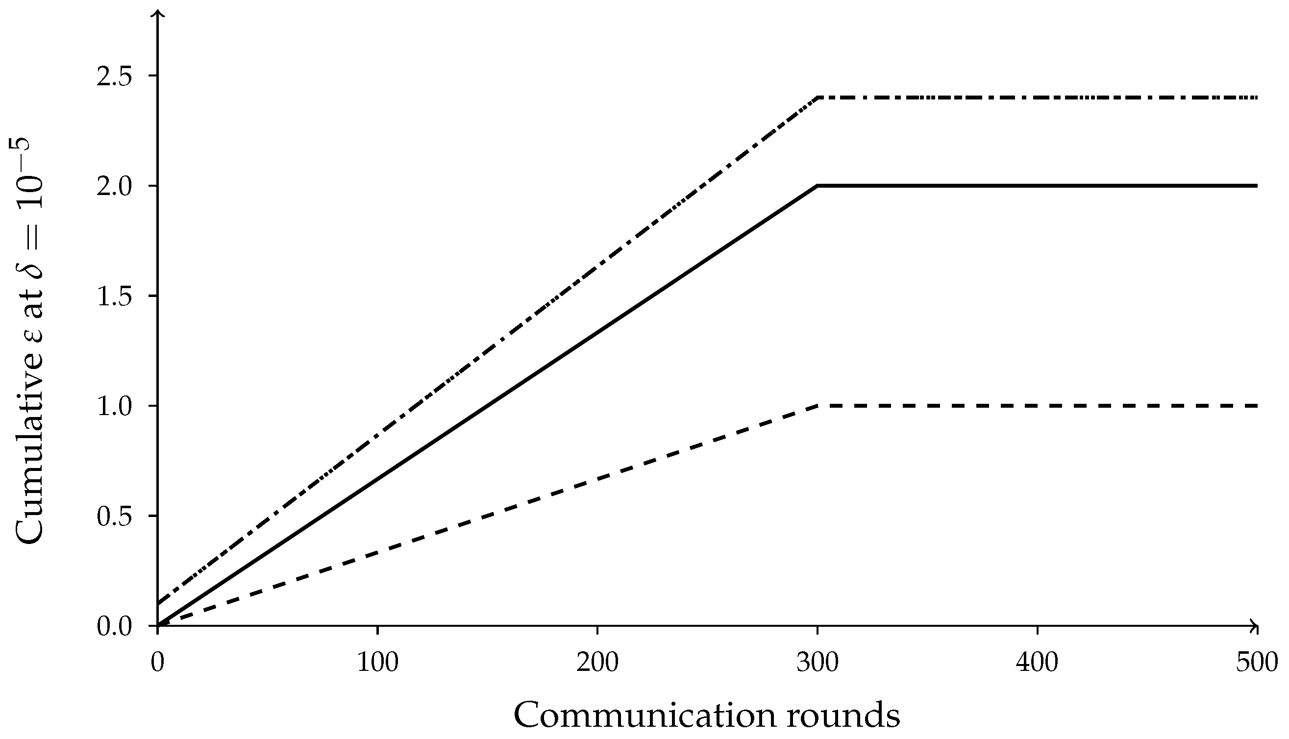
Figure 7.
Privacy budget trajectories. Solid: (weights) under ADDP; dashed: (architecture) under ADDP with uploads every until Phase II at round 300; dotted/dash-dotted: coupled-DP baseline where both channels accrue the same budget more rapidly. No legend is drawn; curve semantics are specified here.
Table 1.
Datasets and client partitions. Each dataset specifies the number of clients N, temporal resolution, train/test spans, input window L, feature dimension d, and median per-client statistics (tickers and train samples). These per-client counts are reported explicitly to facilitate cross-dataset comparison.
| Dataset | N | Resolution | Train Span | Test Span | L | d | Median Tickers/Client | Median Train Samples/Client |
|---|
| Daily-US | 20 | 1 day | 2012–2024 | 2025 | 64 | 32 | 25–30 | ∼80 k sequences |
| Minute-US | 25 | 1 min | 2019–2024 | 2025 | 120 | 40 | 8–10 | ∼2.5 M bars |
| Daily-Global | 18 | 1 day | 2012–2024 | 2025 | 64 | 32 | 20–25 | ∼75 k sequences |
Table 2.
Optimization, privacy, and communication settings. Temperatures anneal : . Architecture uploads occur every rounds. Quantization uses 8-bit stochastic rounding; sparsification keeps top- entries post-clipping.
Table 2.
Optimization, privacy, and communication settings. Temperatures anneal : . Architecture uploads occur every rounds. Quantization uses 8-bit stochastic rounding; sparsification keeps top- entries post-clipping.
| Dataset | K | E | | q | | | Compression |
|---|
| Daily-US | 300 | 5 | 5 | 0.3 | (1.0, 0.2) | (0.75, 1.20) | 8-bit + top-k |
| Minute-US | 600 | 5 | 5 | 0.3 | (1.0, 0.2) | (0.75, 1.20) | 8-bit + top-k |
| Daily-Global | 300 | 5 | 5 | 0.3 | (1.0, 0.2) | (0.75, 1.20) | 8-bit + top-k |
| Dataset | Regimes R | Resource weights | | | | | |
| All | 3 | (1.0, 0.5) | ≈2.0 | ≈1.0 | | | |
Table 3.
Aggregate forecasting and trading metrics on test sets. RMSE (lower is better), DA in %, SR annualized. CIs are client-bootstrapped intervals.
Table 3.
Aggregate forecasting and trading metrics on test sets. RMSE (lower is better), DA in %, SR annualized. CIs are client-bootstrapped intervals.
| Method | Daily-US | Minute-US | Daily-Global |
|---|
|
RMSE
|
DA
|
SR
|
RMSE
|
DA
|
SR
|
RMSE
|
DA
|
SR
|
|---|
| Local-GRU | 0.0118 | 53.1 | 0.54 | 0.00128 | 52.7 | 0.96 | 0.0103 | 53.4 | 0.62 |
| CI | [0.0116, 0.0120] | [52.3, 53.8] | [0.49, 0.59] | [0.00126, 0.00130] | [52.1, 53.2] | [0.90, 1.01] | [0.0101, 0.0105] | [52.7, 54.1] | [0.58, 0.66] |
| FedAvg-LSTM | 0.0112 | 54.7 | 0.68 | 0.00124 | 53.6 | 1.10 | 0.0099 | 54.2 | 0.74 |
| CI | [0.0110, 0.0114] | [54.1, 55.3] | [0.63, 0.73] | [0.00122, 0.00126] | [53.0, 54.1] | [1.05, 1.15] | [0.0097, 0.0101] | [53.6, 54.8] | [0.70, 0.78] |
| FedProx-Trans | 0.0107 | 56.8 | 0.78 | 0.00116 | 55.3 | 1.28 | 0.0095 | 56.8 | 0.85 |
| CI | [0.0105, 0.0109] | [56.2, 57.4] | [0.73, 0.83] | [0.00114, 0.00118] | [54.7, 55.9] | [1.23, 1.32] | [0.0093, 0.0097] | [56.2, 57.3] | [0.81, 0.89] |
| Centralized-DARTS | 0.0106 | 57.1 | 0.81 | 0.00114 | 55.6 | 1.31 | 0.0094 | 57.2 | 0.88 |
| CI | [0.0104, 0.0108] | [56.5, 57.7] | [0.76, 0.85] | [0.00112, 0.00116] | [55.0, 56.1] | [1.26, 1.36] | [0.0092, 0.0096] | [56.6, 57.8] | [0.83, 0.92] |
| FedRegNAS (ours) | 0.0102 | 59.0 | 0.87 | 0.00110 | 56.9 | 1.41 | 0.0092 | 59.1 | 0.95 |
| CI | [0.0101, 0.0104] | [58.5, 59.5] | [0.83, 0.91] | [0.00108, 0.00112] | [56.4, 57.4] | [1.37, 1.46] | [0.0091, 0.0093] | [58.6, 59.6] | [0.91, 0.99] |
Table 4.
Improvements of FedRegNAS over the strongest federated baseline (FedProx-Trans). Deltas are absolute differences; the rightmost columns report the fraction of clients with under paired tests (RMSE: Diebold–Mariano on squared error; DA/SR: stratified permutation).
Table 4.
Improvements of FedRegNAS over the strongest federated baseline (FedProx-Trans). Deltas are absolute differences; the rightmost columns report the fraction of clients with under paired tests (RMSE: Diebold–Mariano on squared error; DA/SR: stratified permutation).
| | RMSE | DA (pp) | SR | RMSE | DA | SR |
|---|
| Daily-US | | | | 0.72 | 0.68 | 0.63 |
| Minute-US | | | | 0.78 | 0.74 | 0.70 |
| Daily-Global | | | | 0.69 | 0.66 | 0.61 |
Table 5.
Forecasting accuracy (RMSE) and relative improvement. Lower RMSE indicates higher accuracy. Improvements are relative to the strongest federated baseline (FedProx-Trans).
Table 5.
Forecasting accuracy (RMSE) and relative improvement. Lower RMSE indicates higher accuracy. Improvements are relative to the strongest federated baseline (FedProx-Trans).
| Method | RMSE | Improvement vs. FedProx-Trans (%) |
|---|
|
Daily-US
|
Minute-US
|
Daily-Global
|
Daily-US
|
Minute-US
|
Daily-Global
|
|---|
| Local-GRU | 0.0118 | 0.00128 | 0.0103 | −10.3 | −10.3 | −8.4 |
| FedAvg-LSTM | 0.0112 | 0.00124 | 0.0099 | −4.7 | −6.9 | −4.2 |
| FedProx-Trans | 0.0107 | 0.00116 | 0.0095 | 0.0 | 0.0 | 0.0 |
| Centralized-DARTS | 0.0106 | 0.00114 | 0.0094 | +0.9 | +1.7 | +1.1 |
| FedRegNAS (ours) | 0.0102 | 0.00110 | 0.0092 | +4.7 | +5.2 | +3.2 |
Table 6.
Effect of regime cardinality R on forecasting performance for FedRegNAS on Daily-US and Minute-US. Results are averaged over three runs; best values per column are in bold. provides a robust trade-off across datasets.
Table 6.
Effect of regime cardinality R on forecasting performance for FedRegNAS on Daily-US and Minute-US. Results are averaged over three runs; best values per column are in bold. provides a robust trade-off across datasets.
| R | Daily-US | Minute-US |
|---|
|
RMSE
|
DA (%)
|
Sharpe
|
RMSE
|
DA (%)
|
Sharpe
|
|---|
| 2 | 0.134 | 56.1 | 0.62 | 0.149 | 54.3 | 0.55 |
| 3 | 0.132 | 56.9 | 0.67 | 0.146 | 55.2 | 0.59 |
| 4 | 0.129 | 57.8 | 0.74 | 0.142 | 56.0 | 0.66 |
| 6 | 0.128 | 58.0 | 0.76 | 0.141 | 56.3 | 0.68 |
| 8 | 0.131 | 57.2 | 0.71 | 0.144 | 55.8 | 0.64 |
| 10 | 0.133 | 56.8 | 0.69 | 0.146 | 55.5 | 0.61 |
Table 7.
Comparison of KL-barycentric aggregation and simple averaging of architecture logits under non-IID and severely non-IID client partitions on three datasets. KL-based aggregation improves accuracy and reduces the dispersion of client architectures, consistent with more stable behavior under heterogeneity.
| Method | Daily-US | Minute-US | Daily-Global | Avg. JS-Div. |
|---|
|
RMSE
|
DA (%)
|
RMSE
|
DA (%)
|
RMSE
|
DA (%)
|
(All Datasets)
|
|---|
| Simple avg. (non-IID) | 0.132 | 56.3 | 0.145 | 55.1 | 0.138 | 55.8 | 0.21 |
| KL-barycentric (FedRegNAS) | 0.129 | 57.8 | 0.141 | 56.3 | 0.135 | 57.0 | 0.13 |
| Simple avg. (severe non-IID) | 0.134 | 55.7 | 0.147 | 54.5 | 0.140 | 55.1 | 0.24 |
| KL-barycentric (severe non-IID) | 0.130 | 57.1 | 0.142 | 55.8 | 0.136 | 56.2 | 0.15 |
Table 8.
Calibration of differentiable latency and communication proxies against real measurements under different device and network profiles. High correlation and low MAPE support their use as faithful surrogates in the objective.
Table 8.
Calibration of differentiable latency and communication proxies against real measurements under different device and network profiles. High correlation and low MAPE support their use as faithful surrogates in the objective.
| Proxy/Profile | Pearson Correlation | MAPE (%) |
|---|
| Latency proxy vs. measured (GPU + LAN) | 0.95 | 6.1 |
| Latency proxy vs. measured (CPU + LAN) | 0.93 | 7.8 |
| Latency proxy vs. measured (CPU + 4G) | 0.91 | 9.3 |
| Comm. proxy vs. bytes (GPU + LAN) | 0.97 | 4.8 |
| Comm. proxy vs. bytes (CPU + LAN) | 0.96 | 5.4 |
| Comm. proxy vs. bytes (CPU + 4G) | 0.94 | 7.1 |
Table 9.
Volatility-stratified trading performance on Daily-US. FedRegNAS yields higher directional accuracy and Sharpe ratio in both high- and low-volatility regimes, with especially strong improvements during turbulent periods relative to Local-GRU and FedAvg-LSTM.
Table 9.
Volatility-stratified trading performance on Daily-US. FedRegNAS yields higher directional accuracy and Sharpe ratio in both high- and low-volatility regimes, with especially strong improvements during turbulent periods relative to Local-GRU and FedAvg-LSTM.
| Method | High Volatility | Low Volatility |
|---|
|
DA (%)
|
Sharpe
|
DA (%)
|
Sharpe
|
|---|
| Local-GRU | 53.4 | 0.52 | 55.9 | 0.80 |
| FedAvg-LSTM | 54.2 | 0.61 | 56.7 | 0.88 |
| FedRegNAS | 56.9 | 0.87 | 58.3 | 1.04 |
Table 10.
Ablation study on Daily-US. Each variant removes or modifies one key mechanism while preserving all other hyperparameters. RMSE (lower better), DA (%), Sharpe ratio (SR), mean client upload per round (KB), and variance of validation loss.
Table 10.
Ablation study on Daily-US. Each variant removes or modifies one key mechanism while preserving all other hyperparameters. RMSE (lower better), DA (%), Sharpe ratio (SR), mean client upload per round (KB), and variance of validation loss.
| Variant | RMSE | DA (%) | SR | Comm/Round (KB) | Var (loss) |
| FedRegNAS (full) | 0.0102 | 59.0 | 0.87 | 1605 | 1.4 |
| w/o regime gating | 0.0108 | 56.7 | 0.79 | 1605 | 2.8 |
| mean aggregation (no KL) | 0.0106 | 57.4 | 0.82 | 1605 | 2.3 |
| coupled-DP (single noise budget) | 0.0105 | 57.6 | 0.81 | 1605 | 2.5 |
| no trust weighting | 0.0107 | 57.0 | 0.80 | 1605 | 2.9 |
| Variant | RMSE vs. full | DA (pp) | SR | Trust-weight entropy | |
| w/o regime gating | +0.0006 | −2.3 | −0.08 | 0.91 | |
| mean aggregation | +0.0004 | −1.6 | −0.05 | 0.72 | |
| coupled-DP | +0.0003 | −1.4 | −0.06 | 0.80 | |
| no trust weighting | +0.0005 | −2.0 | −0.07 | 1.00 | |
Table 11.
Communication and latency across datasets. Comm/round is mean client uplink after clipping, 8-bit stochastic quantization, and top-k sparsification (). Latency is median on-device forward pass on a mobile-class CPU.
Table 11.
Communication and latency across datasets. Comm/round is mean client uplink after clipping, 8-bit stochastic quantization, and top-k sparsification (). Latency is median on-device forward pass on a mobile-class CPU.
| Method | Daily-US | Minute-US | Daily-Global | | | |
| Comm/round (KB) | Latency (ms) | Comm/round (KB) | Latency (ms) | Comm/round (KB) | Latency (ms) | | | |
| Local-GRU | 0 | 3.9 | 0 | 5.8 | 0 | 3.8 | | | |
| FedAvg-LSTM | 2820 | 4.1 | 3160 | 6.2 | 2750 | 4.0 | | | |
| FedProx-Trans | 5410 | 6.8 | 6220 | 8.1 | 5090 | 6.5 | | | |
| Centralized-DARTS | 0 | 5.7 | 0 | 7.1 | 0 | 5.6 | | | |
| FedRegNAS | 1605 | 3.6 | 1810 | 5.2 | 1530 | 3.5 | | | |
| Method | Daily-US | Minute-US | Daily-Global |
| Uplink stdev | Downlink (KB) | CPU util. (%) | Uplink stdev | Downlink (KB) | CPU util. (%) | Uplink stdev | Downlink (KB) | CPU util. (%) |
| FedAvg-LSTM | 210 | 1180 | 64 | 240 | 1260 | 72 | 205 | 1150 | 63 |
| FedProx-Trans | 380 | 2040 | 78 | 410 | 2190 | 83 | 360 | 1980 | 77 |
| FedRegNAS | 145 | 910 | 57 | 160 | 980 | 66 | 140 | 885 | 56 |
Table 12.
Uplink payload decomposition (Daily-US). Mean KB per round by component for FedRegNAS. Architectural messages are sent every rounds; weight messages are sent every round. Percentages are relative to total mean uplink.
Table 12.
Uplink payload decomposition (Daily-US). Mean KB per round by component for FedRegNAS. Architectural messages are sent every rounds; weight messages are sent every round. Percentages are relative to total mean uplink.
| Component | (post-clip, post-noise) | (active rounds only) | Metadata (IDs, seeds) | Total |
| Size (KB) | 1220 | 310 | 75 | 1605 |
| Share (%) | 76.0 | 19.3 | 4.7 | 100 |
| Setting | | | | |
| Mean uplink (KB) | 1880 | 1605 | 1480 | 1430 |
| (at ) | 1.48 | 1.00 | 0.78 | 0.60 |
| RMSE (test) | 0.0102 | 0.0102 | 0.0103 | 0.0104 |
Table 13.
Centralized sequence-model baselines versus FedRegNAS. Centralized models pool all data and do not respect FL/DP constraints, serving as upper bounds or side benchmarks. FedRegNAS-C denotes the centralized version of the architecture discovered by FedRegNAS, while “FedRegNAS (federated, DP)” is the full privacy-preserving federated method.
| Model | Daily-US | Minute-US |
|---|
|
RMSE
|
DA (%)
|
Sharpe
|
RMSE
|
DA (%)
|
Sharpe
|
|---|
| DeepAR (centralized) | 0.128 | 57.1 | 0.78 | 0.140 | 55.7 | 0.64 |
| N-BEATS (centralized) | 0.127 | 57.6 | 0.80 | 0.139 | 56.0 | 0.67 |
| TFT (centralized) | 0.126 | 58.2 | 0.83 | 0.138 | 56.5 | 0.70 |
| FedRegNAS-C (centralized) | 0.127 | 58.0 | 0.82 | 0.139 | 56.3 | 0.69 |
| FedRegNAS (federated, DP) | 0.129 | 57.8 | 0.76 | 0.141 | 56.3 | 0.68 |
Table 14.
Ablation of regime gating and KL-barycentric aggregation on the Minute-US dataset. Both components contribute to improved performance, and their combination yields the best results, demonstrating stability of the design in a high-frequency, nonstationary scenario.
Table 14.
Ablation of regime gating and KL-barycentric aggregation on the Minute-US dataset. Both components contribute to improved performance, and their combination yields the best results, demonstrating stability of the design in a high-frequency, nonstationary scenario.
| Variant (Minute-US) | RMSE | DA (%) | Sharpe |
|---|
| No regime gating, no KL (FedAvg logits) | 0.146 | 55.0 | 0.60 |
| Regime gating only | 0.143 | 55.7 | 0.64 |
| KL aggregation only | 0.143 | 55.9 | 0.65 |
| Full FedRegNAS (gating + KL) | 0.141 | 56.3 | 0.68 |
Table 15.
Training-time comparison and amortization for FedRegNAS and fixed-architecture FL baselines on Daily-US. The one-time NAS search is more expensive, but when amortized across multiple markets or retraining periods, the effective per-deployment cost approaches that of FedProx-Trans.
Table 15.
Training-time comparison and amortization for FedRegNAS and fixed-architecture FL baselines on Daily-US. The one-time NAS search is more expensive, but when amortized across multiple markets or retraining periods, the effective per-deployment cost approaches that of FedProx-Trans.
| Method | Time (h) | GPU-h | Amortized (3 Dep., GPU-h) |
|---|
| FedAvg-LSTM | 8.1 | 32 | 32 |
| FedProx-Trans | 10.4 | 41 | 41 |
| FedRegNAS (search + train) | 24.6 | 98 | ≈33 |
| FedRegNAS (fine-tune only) | 9.0 | 36 | ≈33 |
Table 16.
Performance of different methods in the simulated institutional scenario on Minute-US. All metrics are computed after enforcing regulatory windows and trading constraints. FedRegNAS attains the highest directional accuracy and Sharpe ratio while keeping turnover and pre-clipping constraint violations at or below the levels of FL baselines.
| Method | DA (%) | Sharpe | Avg. Turnover (%/day) | Constraint Violations (%) |
|---|
| Local-GRU | 54.1 | 0.58 | 12.4 | 3.9 |
| FedAvg-LSTM | 55.0 | 0.62 | 11.8 | 3.2 |
| FedProx-Trans | 55.6 | 0.66 | 11.5 | 2.8 |
| FedRegNAS | 56.4 | 0.73 | 11.2 | 2.1 |
Table 17.
End-to-end inference latency per prediction under the simulated institutional setup, including communication and decoding, measured across clients on a heterogeneous GPU/CPU cluster. All methods satisfy the 10 ms mean-latency budget; FedRegNAS remains competitive with FedAvg-LSTM and improves on FedProx-Trans despite performing federated NAS.
| Method | Mean Latency (ms) | 95th Percentile Latency (ms) | Budget Satisfied (≤10 ms Mean) |
|---|
| Local-GRU | 7.6 | 9.8 | Yes |
| FedAvg-LSTM | 8.3 | 10.5 | Yes |
| FedProx-Trans | 9.4 | 11.9 | Yes |
| FedRegNAS | 8.7 | 10.8 | Yes |
