Joint Routing Optimization of Autonomous Vehicles Under Recharging and Battery-Swapping Modes

Abstract

Recharging and battery swapping are of great significance for extending the driving range of autonomous vehicles (AVs). However, if an AV cannot recharge or swap batteries in a timely manner, the consequences are more serious than for a traditional human-driven vehicle, as there is a lack of human assistance in an AV. To address this challenge, this study proposes the joint routing optimization of AVs under recharging and battery-swapping modes. Firstly, a multi-objective model is defined for the joint routing optimization problem of AVs, which minimizes the total distance, idling time, and charging waiting time of AVs while meeting all user demands. The user demand is described as a directed arc consisting of a departure node and a destination at random locations and times, and the AVs need to plan their routes to sequentially access all user demand arcs and recharge or swap batteries in a timely manner. Secondly, an improved artificial plant community (APC) algorithm is proposed to solve the NP-hard problem, including a recharging scheme and a hybrid scheme comprising recharging and swapping. In the seeding operation, random seeds are generated to enhance global search capabilities, and optimal solution learning is added in the fruiting operation to improve local search capabilities. In the growing operation, population optimization is strengthened to improve convergence performance. Thirdly, a benchmark test set was developed based on a real scenario in Wuhan, China. Compared to some baseline algorithms, the results show that the proposed APC algorithm exhibits better performance in solving the NP-hard problem.

1. Introduction

The autonomous vehicle (AV) [1], also known as the intelligent vehicle, autonomous electric vehicle (AEV) [2], driverless vehicle (DV) [3], computer-driven car, or wheeled mobile robot, is the future development direction of the automobile industry and a revolutionary means of transportation. It realizes driverless operation through a computer system [4]. Recent operational experience has shown that AVs have strong advantages in providing mobility-on-demand (MoD) services for citizens [2], including late-night commuting, adverse weather conditions, peak-hour travel, and service to public transportation blind spots [5]. Due to their limited battery capacity, AVs require regular recharging or battery swapping to extend their driving range, but the recharging or swapping process can also introduce challenges when providing mobility-on-demand services to citizens [6].

To address this challenge, existing research has attempted different methods and achieved certain results: deep learning (DL)-based trajectory tracking methods [3], trajectory planning algorithms [4], time-dependent vehicle routing problems [5], recharging and transportation scheduling under the swapping mode [6], autonomous vehicle trajectory prediction [7], autonomous vehicle path planning [8], and a vehicle-on-demand system [9]. Mobility on demand is a mode of providing point-to-point transportation services through shared vehicles (such as taxis, shared bicycles, etc.) [2,9], allocating vehicles in real-time based on passenger demand, reducing idling rates, and alleviating urban traffic pressure. The authors of [4] reviewed 226 references and conducted a survey on autonomous vehicle behaviors. Their study discussed the current challenges and future prospects of trajectory planning tasks in autonomous vehicles, but the influence of the charging or battery-swapping process on the trajectory of the autonomous vehicle was ignored.

However, the limited battery capacity and speed constraints of AVs necessitate frequent charging, which is significantly more time-consuming than the traditional fuel refilling process [2,10]. In recent years, related research has mainly focused on the field of electric vehicles (EVs) rather than autonomous vehicles [11]. Although the deployment of more charging stations (CSs) and higher-cost battery-swapping stations can effectively relieve the charging pressure of AVs, these stations require a substantial investment, and the charging behavior of AVs cannot be completely avoided, especially in big cities. Some approaches leverage artificial intelligence (AI) technologies [1], such as neural computing or metaheuristic algorithms, to solve challenges: the DL approach [3]; improved artificial potential field [8]; genetic algorithm (GA) [10]; distributed generation (DG) [12]; probabilistic self-adjusted modified particle swarm optimization (SAPSO) algorithm [12]; multi-agent deep reinforcement learning (DRL) [13]; and Lagrange relaxation algorithm [14]. Among these, the evolutionary algorithm is a general framework that balances global search and local optimization by simulating natural phenomena or introducing random strategies, and it is better at finding global optimal solutions, especially for vehicular edge computing platforms with limited computing resources and power.

On the one hand, recharging or battery swapping for AVs can reduce human intervention and increase the range of AVs. On the other hand, when no one intervenes, failures in the recharging or battery-swapping process can result in more serious problems than those encountered with manned vehicles. However, there is very little research on the challenges in this area. In this study, our research motivation is to jointly optimize the routing of AVs under recharging and battery-swapping modes. In order to solve such complex problems on AVs’ edge computing platforms, an improved artificial plant community (APC) algorithm [15] was developed. The primary contributions of this study are as follows:

• Compared to existing research, this study is the first to solve the joint routing optimization problem of AVs under recharging and battery-swapping modes. The system is defined as a multi-objective routing optimization model with a demand diagram, where a user demand includes a directed arc composed of a departure node and a destination at random locations and times, and the recharging demand or battery-swapping demand is an independent station node. The goal is to meet all user demand arcs and necessary recharging or battery-swapping demands within the deadline while minimizing the total distance, idling time, and charging waiting time for AVs.
• An improved artificial plant community algorithm is proposed to solve the NP-hard problem, including a recharging scheme and a hybrid recharging and swapping scheme. In the seeding operation, random solutions were added to enhance global search capability, and the mutation of the optimal solution was added in the fruiting operation to increase local search capabilities. In the growing operation, population selection was strengthened to enhance convergence ability.
• A benchmark test set was developed based on a real scenario in Wuhan, China, with a great demand for AVs and a small number of charging stations and battery-swapping stations. The user demand arcs are random, but they follow a non-uniform distribution between densely populated urban areas and sparsely populated suburban areas. The results show that the proposed APC algorithm has better performance than some baseline algorithms.

The remainder of this study is structured as follows. Section 2 provides a review of related research. Section 3 discusses the joint routing optimization model of AVs. In Section 4, an evolutionary algorithm is introduced for AV routing. The results are detailed in Section 5. Finally, Section 6 concludes this study.

2. Related Research

The user service response and recharging of autonomous vehicles are two major problems that hinder their development [2], and these two sub-problems are closely related. Obtaining the optimal solution of one of the sub-problems alone cannot result in the optimal solution of the global problem.

Existing research has mainly focused on the impact of recharging in electric vehicles on driving trajectories and user services. The authors of [9] defined the MoD problem via a mixed-integer linear program (MILP) formulation and presented a set of intelligent and efficient heuristic algorithms to solve it. The authors of [16] optimized the electric vehicle routing problem with pickup and delivery under the partial recharging and nonlinear discharging strategy. The authors of [17] modeled the mobility-aware charging scheduling as a partially observable Markov decision process (POMDP) and developed deep reinforcement learning (DRL) combined with binary linear programming (BLP) to search for a near-optimal solution. The authors of [18] described the on-demand charging and battery degradation strategy as a mixed-integer nonlinear programming (MINLP) model with a piecewise linear approximation approach and outer-approximation method to linearize the proposed model. The authors of [19] introduced an on-demand shared autonomous electric vehicle (SAV) service and coupled charging and repositioning events to improve service quality, reduce empty travel, and enhance fleet utilization.

Some scholars believe that optimizing the path of electric vehicles is NP-hard when considering both service demands and recharging demands simultaneously, and traditional algorithms struggle to solve this issue. The authors of [20] considered the routing problem between multiple MoD-EV stations as a multi-server queuing system, and they formulated the jointly minimizing problem of the average trip time for all users and the average charging cost as a dual-objective convex optimization problem. The authors of [21] investigated electric vehicle routing problems (EVRPs) with recharging policy, considering the limited range of electric vehicles. The authors of [22] introduced branch-price-and-cut algorithms for the electric vehicle routing problem with heterogeneous recharging technologies and nonlinear recharging functions. The authors of [23] believed that such issues are a multi-objective electric vehicle routing problem with five conflicting objectives: the total minimization cost of recharging, number of vehicles required, total travel distance, load-dependent energy consumption, and total number of charging stations required. The authors of [24] described this issue as a multi-depot electric vehicle routing problem (MDEVRP). Unreasonable charging planning will result in AV loading defects [23,24].

In addition to charging technology, battery-swapping technology can also extend the driving range of electric vehicles while also affecting their driving trajectory. The authors of [14] optimized highway electric vehicle scheduling and battery-swapping station management for enhanced renewable energy utilization. The authors of [25] published a note on battery-swapping policies in the electric vehicle routing problem with time windows and battery-swapping vehicles. The battery-swapping process often consumes less time than the recharging process, but fewer battery-swapping stations also make route planning more challenging. In metropolitan areas, limited space makes constructing new charging facilities a major concern—let alone higher-cost battery-swapping stations; thus, reasonable charging planning is of great significance for optimizing service response. The authors of [6] proposed recharging and transportation scheduling for electric vehicle batteries under the swapping mode. The authors of [11] developed the joint distribution route optimization of fresh supplies via electric vehicles under charging and battery-swapping modes.

Recent studies tend to utilize existing infrastructure on AV charging patterns to develop scheduling strategies, such as predicting EV charging demands in renewable-energy-powered grids using explainable machine learning [26]. In practical applications, AV energy consumption is also affected by vehicle speed or other factors [27]. Many AI algorithms and evolutionary algorithms typically have good approximate solutions for all types of problems, as they ideally do not make any assumptions about the underlying fitness [1]. Common algorithms include the following: GA [10,24], PSO algorithm [12,28], artificial physarum polycephalum colony (APPC) [29], APC algorithm [15,30], offline–online heuristic algorithm (OOHA) [22], hybrid ant colony optimization (HACO) [23], artificial bee colony algorithm (ABCA) [23], differential evolution (DE) [28], whale optimization algorithm (WOA) [28], and gray wolf optimizer (GWO) [28]. Machine learning and deep learning are developed based on algorithm models such as artificial neural networks, and they have the ability to automatically extract features. They have also received widespread attention in recent years, such as DL [3], machine learning (ML) [26], graph convolutional networks [31], the attention-based graph learning approach [32], and DRL [13,17,33].

The above body of research demonstrates the following research gaps.

First, the charging and battery-swapping processes of the autonomous vehicle have a significant impact on its driving trajectory and could result in more serious consequences than traditional human-driven electric vehicles without intervention. There are few solutions to such joint optimization problems in existing research.

Second, the edge computing platform of AVs has limited computing resources and power. Methods for deploying efficient algorithms on the edge computing platform of AVs to solve the above problems are extremely challenging.

Third, there is a lack of suitable datasets for benchmarking or training machine learning and deep learning.

Our research attempts to address the aforementioned research gaps.

3. Materials and Methods

In this section, we outline the mathematical modeling used in this study for the joint routing optimization problem of AVs under recharging and battery-swapping modes.

3.1. Symbol Definition

The symbols used in this study are defined in Table 1.

Table 1. Symbol definitions.

Symbol	Definition	Measurement Unit
${a(a}_x,a_y)$	Node identification with its latitude and longitude coordinates	km
$d_{a,b}^{min}$	The shortest distance between two nodes ${a(a}_x,a_y)$ and ${b(b}_x,b_y)$	km
$d_i^{total}$	The total distance of AV $v_i$	km
$e_{a,b}(t)$	An edge from the departure node ${a(a}_x,a_y)$ to the destination node ${b(b}_x,b_y)$ at time $t$	km
$t$	Time variable	hour
$T$	Total operating cycle	hour
$t_{a,b}^{ddl}$	The demanded deadline	hour
$D_{a,b}(t)$	A demand from the departure node ${a(a}_x,a_y)$ to the destination node ${b(b}_x,b_y)$ at time $t$	-
$t^{start}$	The lowest start time among all demands	hour
$t^{ddl}$	Overall deadline	hour
$v_i$	Index of an AV	-
$a_{max}$	Total number of nodes	-
$v_{max}$	Total number of AVs	-
$r_i^{travel}$	Average travel speed of AV $v_i$	km/hour
$r_i^{travelm}$	Maximum travel speed of AV $v_i$	km/hour
$r_i^{charge}$	Charging rate of AV $v_i$ per time unit	A
$r_i^{discha}$	Discharging rate of AV $v_i$ per distance unit	A
$b_i^{max}$	Maximum battery capacity of AV $v_i$	A·hour
$b_i^{min}$	Minimum remaining energy of battery required for AV $v_i$	A·hour
$b_i^{age}$	The battery degradation coefficient for AV $v_i$	%
$u_i^{run}(t)$	Binary running state of AV $v_i$ at time $t$	Boolean
$u_i^{charge}(t)$	Binary charging state of AV $v_i$ at time $t$	Boolean
$u_i^{waitc}(t)$	Binary waiting state of AV $v_i$ for a charge	Boolean
$u_i^{waitd}(t)$	Binary waiting state of AV $v_i$ for a demand	Boolean
$t_i^{run}$	Running time of AV $v_i$ at time $t$	hour
$t_i^{charge}$	Charging time of AV $v_i$ at time $t$	hour
$t_i^{discha}$	Discharging time of AV $v_i$ at time $t$	hour
$t_i^{waitc}$	Charging waiting time of AV $v_i$ for a charge	hour
$t_i^{waitd}$	Demand waiting time of AV $v_i$ for a demand	hour
${\lambda }_{iab}$	Binary selection bit of AV $v_i$ on edge $e_{a,b}(t)$	Boolean
$t_{iab}$	The travel time of AV $v_i$ on edge $e_{a,b}(t)$	hour
$t_i^{idl}$	The idling time of AV $v_i$	hour
$k_c$	Available charging stations on node ${c(c}_x,c_y)$
$k_s$	Available swapping stations on node ${s(s}_x,s_y)$
$S$	Population size of the APC
$x$	A feasible solution
$I$	Iteration
$p_{seed}$	The seeding probability
$p_{grow}$	The growing probability
$p_{fruit}$	The fruiting probability
$fitness$	The fitness function

The demand graph is considered as a directed graph $G(V,E)$, where $V$ represents the set of nodes, and $E$ represents the direct paths between these nodes. A node may be a user node or a charging station node. There are two types of demands: user demands and/or battery-swapping demands. Each user or charging station node corresponds to a node identification ${a(a}_x,a_y)$ with its latitude and longitude coordinates. Then, the shortest distance between two nodes ${a(a}_x,a_y)$ and ${b(b}_x,b_y)$, (a, b $\in$ V), is denoted as $d_{a,b}^{min}$:

$$d_{a,b}^{min}=\sqrt{{\left(a_x-b_x\right)}^2{+(a_y-b_y)}^2}.$$

(1)

The distance between two nodes is simplified as the Euclidean distance, which may be different compared to the actual Manhattan distance or road network distance in urban environments. However, they can all be described as line segments of a certain length. Then, a user demand $D_{a,b}(t)$ can be defined by the tuple ⟨$e_{a,b}(t)$, $t_{a,b}^{ddl}$⟩, where $e_{a,b}(t)$ is an arc from the departure node ${a(a}_x,a_y)$ to the destination node ${b(b}_x,b_y)$ at time $t$, and $t_{a,b}^{ddl}$ is the demand’s deadline.

Users can hire AVs and drop them off at their respective destination nodes upon completion of use. Each AV $v_i$ $\in$ $v_{max}$ is characterized by its average travel speed $r_i^{travel}$, maximum battery capacity $b_i^{max}$, charging rate $r_i^{charge}$, and discharging rate $r_i^{discha}$. At any time t $\in$ $T$, AV $v_i$ can be in one of four binary states: running on demand ($u_i^{run}(t)$), charging at a charging station ($u_i^{charge}(t)$), waiting for a charge ($u_i^{waitc}(t)$), or waiting for a new demand ($u_i^{waitd}(t)$). Therefore, we have

$$u_i^{run}\left(t\right)+u_i^{charge}\left(t\right)+u_i^{waitc}\left(t\right)+u_i^{waitd}\left(t\right)=1.$$

(2)

Based on the four binary states above, all AV routes can be established, where the total distance, idling time, and charging waiting time of AVs can be determined.

3.2. Joint Routing Optimization

A joint routing optimization example of AVs in a simple road network is depicted in Figure 1, where there is a departure node ($a$) and a destination ($b$), in addition to a charging station ($c$) and a battery-swapping station ($s$). The edges ${\{e}_{a,b}\}$ in this graph are weighted according to the distance between these nodes, which can be calculated using Equation (1). $d_{a,b}^{min}$ is used to denote the shortest path between nodes a and b.

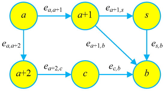
Figure 1. A joint routing optimization example of AVs.

For the sake of analysis, the following assumptions are made.

A1: The user’s demands are assumed to be independent and without interference from each other. The situation where users temporarily modify the departure node and destination is not considered.

A2: The capacity of all charging stations or battery-swapping stations is assumed to be sufficient; insufficient charging power or battery shortage situations are not considered.

A3: Assuming that an edge travels in any direction, its weight, i.e., the shortest distance, is fixed and unchanging. We do not consider the possibility that the distances between two nodes may differ depending on the direction of travel.

A4: All AVs are assumed to be homogeneous, without considering differences in meeting user demands. Every AV can meet the demands of all users.

A5: All batteries used by AVs are assumed to be homogeneous, without considering battery differences between AVs.

In Figure 1, there is a demand for AVs on node $a$ at t = 0, destined for $b$ with a deadline of $t_{a,b}^{ddl}$. Figure 1 shows three paths from $a$ to $b$: Path 1 $(a \to a+1 \to s \to b)$, with a distance of $(d_{a,a+1}^{min}+d_{a+1,s}^{min}+d_{s,b}^{min})$; Path 2 $(a \to a+1 \to b)$, with a distance of $(d_{a,a+1}^{min}+d_{a+1,b}^{min})$; and Path 3 $(a \to a+2 \to c \to b)$, with a distance of $(d_{a,a+2}^{min}+d_{a+2,c}^{min}+d_{c,b}^{min})$. An AV can choose Path 1 and swap the battery midway, which will increase the travel range, but it will have sufficient power to respond to the next user demand after reaching destination ($b$). If Path 2 is selected without any recharging or battery swapping, an AV will reach its destination in the shortest possible time, but due to power consumption, it will have difficulty responding to subsequent user demands. An AV can also choose Path 3 and recharge midway, but this requires longer waiting times for recharging. After reaching its destination, it will have sufficient power to respond to subsequent user demands. However, by combining and optimizing various path strategies, the deadline for the required AVs can be greatly shortened.

For joint routing optimization, the binary selection bit ${\lambda }_{iab}$ of AV $v_i$ on edge $e_{a,b}(t)$ could be set to 1 to indicate that AV $v_i$ selects edge $e_{a,b}(t)$; otherwise, ${\lambda }_{iab}=0$. Equation (3) defines the non-negativity of the travel time $t_{iab}$ of AV $v_i$ on edge $e_{a,b}(t)$, and indicates that the limitation of the travel time $t_{iab}$ should meet user demands:

$${\forall t_{iab}{\lambda }_{iab}\ge 0,t}_{iab}\in \left[t_{a-1,a}^{ddl},t_{a,b}^{ddl}\right]$$

(3)

In joint routing optimization, Equations (4)–(6) constrain the value of ${\lambda }_{iab}$ to be in the range of 0 to 1. Equation (4) ensures that an AV only has one start node. Equation (5) guarantees a continuous path. Equation (6) ensures that there is only one end node or one exit:

$${\sum }_c{u_i^{run}\left(t\right)\lambda }_{iac}-{\sum }_c{u}_i^{run}\left(t\right){\lambda }_{ica}=1,\left(c\in V,c\ne a\right)$$

(4)

$${\sum }_{a,c}{u_i^{run}\left(t\right)\lambda }_{iac}-{\sum }_{c,d}{u_i^{run}\left(t\right)\lambda }_{icd}=0, \left(c,d\in V;c,d\ne a,b\right)$$

(5)

$${\sum }_c{u}_i^{run}\left(t\right){\lambda }_{icb}-{\sum }_c{u}_i^{run}\left(t\right){\lambda }_{ibc}=1,\left(c\in V,c\ne b\right)$$

(6)

Equation (7) determines that the average travel speed $r_i^{travel}$ of AV $v_i$ can be obtained through the travel distance $d_{a,b}^{min}$ and time $t_{iab}$, and it cannot be higher than the maximum travel speed of $r_i^{travelm}$:

$$r_i^{travel}={\displaystyle \frac{d_{a,b}^{min}}{t_{iab}}}\le r_i^{travelm}$$

(7)

Let $b_i^{max}$ denote the maximum battery capacity of AV $v_i$. Consequently, the minimum remaining energy of the battery ($b_i^{min}$) required for AV $v_i$ to be considered available at time t is given by

$$b_i^{min}=\mathit{min}\{\left(\mathit{max}\left\{d_{a,b}^{\mathit{min}}\right\}\times r_i^{discha}\right),b_i^{age}{b}_i^{max}\},$$

(8)

where $d_{a,b}^{min}$ represents the shortest distance between $a$ and $b\in V$ (the node set). The battery degradation coefficient, $b_i^{age}\in \left[\mathrm{0,1}\right]$, is related to the recharging rate, number of recharging cycles, and duration of use.

Thus, to ensure that AV $v_i$ is available on node $a$, it must have sufficient power and meet the following constraint:

$$b_i^{max}+{\sum }_{t^{\prime }=1}^t\left(\begin{array}{c}{u}_i^{waitc}\left(t^{\prime }\right)\times r_i^{charge}\\ -u_i^{run}\left(t^{\prime }\right) \times r_i^{travel}\times r_i^{discha}\end{array}\right)\ge b_i^{min}.$$

(9)

According to Equation (9), the travel distance between any two adjacent nodes in the network must be within the maximum distance of an AV. This can be determined by the maximum battery capacity $b_i^{max}$ of AV $v_i$ and the discharging rate $r_i^{discha}$ of AV $v_i$ per unit distance:

$$d_{a,b}\le b_i^{max}/r_i^{discha}$$

(10)

In total operating cycle $T$ $\in$ [$t^{start}$, $t^{ddl}$], $t^{start}$ is the earliest start time among all demands, and $t^{ddl}=\mathit{max}(t_{a,b}^{ddl})$∀$D_{a,b}(t)$ is the overall deadline. Since time t $\in$ $T$, we obtain $T$ = $t^{start}$, $t^{start}+1$, …, $t^{ddl}$. The total travel time of AV $v_i$ from a departure node to a destination includes travel, waiting, and charging times, all of which must be completed within the deadline. Hence, we have the following:

$$t_{iab}=u_i^{run}\left(t\right)t_i^{run}+u_i^{charge}\left(t\right)t_i^{charge}+u_i^{waitc}{\left(t\right)t}_i^{waitc}+u_i^{waitd}{\left(t\right)t}_i^{waitd}.$$

(11)

The time taken to travel for a demand $D_{a,b}(t)$ via the shortest path by AV $v_i$ must not exceed the deadline, which is expressed as Equation (12):

$$t_i^{run}=d_{a,b}/r_i^{travel}\le t_{a,b}^{ddl}$$

(12)

Equation (13) limits the charging time $t_i^{charge}$ of AV $v_i$, i.e., the sum of the charging time of AV $v_i$ at all charging stations. At the same time, Equations (8) and (9) jointly limit the remaining power and electricity that needs to be charged.

$$t_i^{charge}={\sum }_c{\displaystyle \frac{r_i^{discha}{d}_{a,c}}{r_i^{charge}}}\le t_{a,b}^{ddl}$$

(13)

The charging waiting time of AV $v_i$ for a charge via the shortest path by AV $v_i$ must not exceed the maximum travel speed of AV $v_i$, as shown in Equation (14):

$$t_i^{waitc}=d_{a,c}/r_i^{travel}\ge d_{a,c}/r_i^{travelm},$$

(14)

if node c is a charging station.

The demand waiting time of AV $v_i$ for a demand via the shortest path by AV $v_i$ must not exceed the difference between the two deadlines, which can be obtained via Equation (15):

$$t_i^{waitd}=t_{a,b}^{ddl}-t_{a-1,a}^{ddl}\le d_{a-1,a}/r_i^{travel}$$

(15)

3.3. Multi-Objective Routing Optimization Function

The goal of joint routing optimization is to meet all demands within their deadlines while minimizing the total distance, idling time, and charging waiting time of the AVs.

Firstly, the total distance is the first objective in the joint routing optimization problem, which refers to the travel distance of all AVs. According to $d_{a,b}^{min}$ in Equation (1), $u_i^{run}\left(t\right)$ in Equation (2), and ${\lambda }_{iab}$ in Equation (3), the total distance of AV $v_i$ can be obtained:

$$d_i^{total}={\sum }_{a,b}{u_i^{run}\left(t\right)\lambda }_{iab}{d}_{a,b}^{min}$$

(16)

Secondly, the idling time is the second objective in the joint routing optimization problem, which refers to the duration of vehicle travel without passengers. According to Equations (13) and (14), the idling time of AV $v_i$ can be calculated by the sum of the idling times of AV $v_i$ at all nodes.

$$t_i^{idl}={\sum }_b(t_i^{waitc}+t_i^{waitd})$$

(17)

Then, the total idling time can be determined by the maximum idling time of all AVs.

$${\sum }_i{t}_i^{idl}=\underset{i}{\mathit{max}}({\sum }_b{(t}_i^{waitc}+t_i^{waitd}))\le t^{ddl}-t^{start}$$

(18)

In the scenario where there is no delay between a demand’s arrival and the assignment of an AV to meet that demand, the demands are addressed by an AV immediately, i.e., there is less idling time:

$$\underset{i}{\mathit{min}}(t_i^{waitc}+t_i^{waitd})\le t_{a,b}^{ddl}$$

(19)

According to Equation (19), the available vehicles with less idling time at any given moment during the scheduling period $T$ should be prioritized to meet joint routing optimization across all charging stations.

Thirdly, the charging waiting time is the third objective in the joint routing optimization problem. Each node $c$ has a variable $k_c$, indicating the number of available charging stations, with $k_c$ = 0 signifying that charging is unavailable at that node. The total number of vehicles that can be charging at any time is limited to the total number of charging stations available within the network:

$${\sum }_{i=0}^{i_{max}}{\lambda }_{iac}(t)\le {\sum }_{c\in V,k_c>0}{k}_c.$$

(20)

Here, ${\lambda }_{iac}=1$ means that charging station $c$ is ready for charging, while ${\lambda }_{iac}=0$ means that the charging station is not ready for charging. The total number of available or occupied charging stations can be calculated via the sum ${\sum }_{i=0}^{i_{max}}{\lambda }_{iac}(t)$. AV $v_i$ should wait on node $c$ at time t if all charging stations are occupied, i.e., ${\sum }_{i=0}^{i_{max}}{\lambda }_{iac}\left(t\right)=\sum _{c\in V,k_c>0}{k}_c$. In cases where ${\sum }_{i=0}^{i_{max}}{\lambda }_{iac}\left(t\right)<\sum _{c\in V,k_c>0}{k}_c$, there are available charging stations to accommodate the charging demand.

According to Equation (14), the total charging waiting time can be determined by the maximum charging waiting time of all AVs.

$${\sum }_i{t}_i^{waitc}=\underset{i}{\mathit{max}}({\sum }_c{d}_{a,c}/r_i^{travel})$$

(21)

According to the total distance in Equation (16), the total idling time in Equation (17), and the total charging waiting time in Equation (21), the joint routing optimization problem of AVs under recharging and battery-swapping modes can be expressed as

$$\begin{gathered} obj=\{min\left({\sum }_i{d}_i^{total}\right),min\left({\sum }_i{t}_i^{idl}\right),min\left({\sum }_i{t}_i^{waitc}\right)\}. \\ St.Equations \left(3\right)-\left(15\right). \end{gathered}$$

(22)

In the multi-objective function, there are many constraints. Equation (3) constrains the binary selection bit, ${\lambda }_{iab}$ of AV $v_i$. Equation (4) only constrains one start node. Equation (5) constrains a continuous path. Equation (6) constrains only one end node or one exit. Equation (7) constrains the average travel speed $r_i^{travel}$ of AV $v_i$. Equation (8) constrains the minimum remaining energy of the battery ($b_i^{min}$) required for AV $v_i$. Equation (9) constrains the minimum remaining energy of the battery on a node. Equation (10) constrains the travel distance between any two adjacent nodes. Equation (11) constrains the total travel time of AV $v_i$ from a departure node to a destination. Equation (12) constrains the travel time for a demand $D_{a,b}(t)$. Equation (13) constrains the charging time $t_i^{charge}$ of AV $v_i$. Equation (14) constrains the charging waiting time of AV $v_i$ for a charge. Equation (15) constrains the charging waiting time of AV $v_i$ for a charge.

4. An Improved APC Algorithm

It is apparent that Equation (22) is NP-hard, and it is challenging to search for an optimal solution for large AV networks with numerous uncertain demands. Thus, in this section, an improved APC algorithm is developed to quickly achieve optimal results. Specifically, its global search capability and local search capability are enhanced.

4.1. Improved Search Mechanism

The process of our APC algorithm comprises five main steps, i.e., initialization, seeding, growing, fruiting, and end judgment. The first initialization stage is to set the main parameters and the objective function of joint routing optimization, and the original population of the APC is randomly generated in this stage. The second seeding stage is improved to generate many feasible APC solutions for a heuristic search. The third growing stage is improved to select the optimal solutions to the joint routing optimization problem. The fourth fruiting stage is improved to search for the local optimal solutions. Finally, the end judgment stage is designed to determine whether the evolutionary computation has finished and to output the optimal solution.

Step 1—Initialization: The first step prepares two main parameters: the demand graph and the APC.

A demand graph can be modeled as a directed graph $G\left(V,E\right)$ with a node set ${\{a(a}_x,a_y)\}$ and an edge set ${\{e}_{a,b}(t)\}$. There is a total number ($a_{max}$) of nodes in the node set, where a pair of coordinates of node $a$ is ${(a}_x,a_y)$. Then, a distance matrix ${\{d}_{a,b}^{min}\}$ is used to connect these nodes, where $d_{a,b}^{min}$ is the shortest distance on edge $e_{a,b}(t)$. The demand set is ${\{D}_{a,b}(t)\}$, consisting of a departure node and a destination, and the demand’s deadline set is ${\{t}_{a,b}^{ddl}\}$. For AVs, the initialization parameters include the total number $v_{max}$, maximum travel speed $r_i^{travelm}$, charging rate $r_i^{charge}$, discharging rate $r_i^{discha}$, maximum battery capacity $b_i^{max}$, and minimum required battery capacity $b_i^{min}$. The available charging stations on nodes are ${\{k}_c\}$, and the objective function is Equation (22). Hence, the fitness of the APC can be determined using $obj$ in Equation (22), and it is defined as follows from the beginning:

$$fitness=-obj$$

(23)

The initialization parameters of the APC include the population size $S$ of the APC, the seeding probability $p_{seed}$, the growing probability $p_{grow}$, and the fruiting probability $p_{fruit}$. Each artificial APC individual can be randomly initialized as a binary string $x$ encoded by the binary selection bits of AV $v_i$ on edge $e_{a,b}(t)$:

$$x=\{{\lambda }_{iab}\}$$

(24)

As an evolutionary algorithm, the solutions of the APC algorithm are not related to the initialization values; they depend on the evolutionary process. The iteration counter is initialized as 0, and the end judgment conditions should be predefined, i.e., the maximum number of iterations $I_{max}$ and the iteration error threshold $e_{th}$. These parameters determine whether the iterative calculation of the APC ends or continues.

Step 2—Seeding: The second step randomly generates APC seeds in each iteration.

The global search ability of the APC can be improved by the seeding probability $p_{seed}\in$[0,1], and random seeds $\{x_{seed}^{rand}\left(I\right)\}$ are produced in each iteration for global search in the entire solution space. The fruits ${\{x}_{seed}^{fruit}\left(I-1\right)\}$ in the previous iteration $I-1$ are kept for local searches with a probability of $(1-p_{seed})$. The population $\{x_{seed}(I)\}$ of the seeds in iteration $I$ can be divided into two parts:

$${\{x_{seed}(I)\}}_S={\{x_{seed}^{rand}\left(I\right)p_{seed},x_{seed}^{fruit}\left(I-1\right)(1-p_{seed})\}}_S.$$

(25)

In the first iteration ($I=0$), there are no fruits ($\{x_{seed}^{fruit}\left(I-1\right)\}=\varnothing$); thus, all seeds $\{x_{seed}^{rand}\left(I\right)\}$ are randomly produced. The population size of seeds in iteration $I$ retains the value of $S$.

Step 3—Growing: The third step provides the population selection for the APC algorithm.

The convergence ability of the APC can be strengthened by a growing probability $p_{grow}\in \left[\mathrm{0,1}\right]$ to select the optimal seed $\{x_{seed}(I)\}$. Through the fitness function, $fitness$, in Equation (23), the population size of the growing individuals $\{x_{grow}(I)\}$ decreases to $S{p}_{grow}$:

$${\{x_{grow}(I)\}}_{S{p}_{grow}}=\{x_{seed}(I)|\underset{S{p}_{\mathit{grow}}}{\mathit{max}}fit\left(x_{seed}(I)\right){\}}_{S{p}_{grow}}.$$

(26)

Step 4—Fruiting: The fourth step is to search for the local optimal solutions.

The local search ability of the APC is improved in the fruiting step by a fruiting probability of $p_{fruit}\in \left[\mathrm{0,1}\right]$, which indicates how much original information a parent can retain. In this step, the growing individuals $\{x_{grow}(I)\}$ have more opportunities to generate more solutions $\{x_{fruit}(I)\}$, and the crossing fruits of the growing individuals $\{x_{grow}(I)\}$ are produced. It is assumed that there are two parents, $x_{grow}^a(I)$ and $x_{grow}^b(I)$, and they can produce two fruits as follows:

$$\left\{\begin{array}{c}{x}_{fruit}^{cross}(I)=\{{x_{grow}^a(I)}_{p_{fruit}}//{x_{grow}^b(I)}_{{1-p}_{fruit}}\}\\ x_{fruit}^{cross\prime }(I)=\{{x_{grow}^b(I)}_{p_{fruit}}//{x_{grow}^a(I)}_{{1-p}_{fruit}}\}\end{array}\right..$$

(27)

where ‘//’ denotes the concatenation of two strings.

Now, there are two parts of the fruits: namely, the parthenogenesis fruits of the growing individuals $\{x_{grow}(I)\}$ in Equation (26) with a population size $S{p}_{grow}$ and the crossing fruits $\{x_{fruit}^{cross}(I)\}$ of the parents in Equation (27) with a population size $S{p}_{grow}$. The total population size of the fruits has doubled, and we obtain the following:

$${\{x_{fruit}(I)\}}_{2S{p}_{grow}}=\left\{\{x_{grow}(I){\}}_{S{p}_{grow}},\{x_{fruit}^{cross}(I){\}}_{S{p}_{grow}}\right\}$$

(28)

Step 4—End Judgment: The end conditions of the proposed approach can be judged by a predefined maximum number of iterations ($I_{max}$) or the iteration error threshold ($e_{th}$). If the end conditions are not satisfied, the APC will return to the seeding operation for the next iterative computation. Otherwise, the best solution is output.

The conceptual figure of the improved search mechanism is shown in Figure 2a, where the joint routing optimization problem of AVs under recharging and battery-swapping modes is defined as a multi-objective routing optimization model with demand arcs. The goal is to meet all user demand arcs while minimizing the total distance, idling time, and charging waiting time for AVs. The solving process is mainly implemented through continuous cycles of APC seeding, growing, and fruiting.

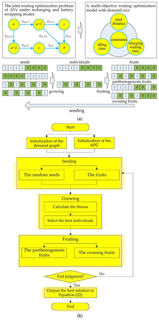
Figure 2. An Improved APC Algorithm. (a) The conceptual figure of the improved search mechanism. (b) APC algorithm flow for the joint routing optimization problem.

The algorithm’s flow is summarized in Figure 2b, including five primary steps to solve the joint routing optimization problem: initialization, seeding, growing, fruiting, and end justification.

In Figure 2b, seeding, growing, and fruiting form a large loop. Before the loop, the related parameters are initialized, and the initial solutions are randomly generated. In the seeding step, the APC produces random individuals to search for the optimal solutions through global search, and the population size retains the original value, $S$. In the growing stage, the APC selects individuals with higher fitness for the next iterations, and the population size decreases to $S{p}_{grow}$. In the fruiting stage, the APC generates more individuals through local search, and the population size increases to $2S{p}_{grow}$. After many iterations, it is possible to find the optimal solutions to the objective function in Equation (22).

Since each artificial APC individual $x$ is encoded by the binary selection bits of AV $v_i$ on edge $e_{a,b}(t)$ for parallel computing, the computational complexity of the proposed APC algorithm is linearly influenced by the number of nodes and AVs. If the maximum number of nodes is $a_{max}$ and the maximum number of vehicles is $v_{max}$, the time complexity of this algorithm is $O(a_{max} v_{max})$.

The subsequent subsections provide the application and corresponding pseudocode of the APC algorithm in two different scenarios: one is the recharging scheme, and the other is a hybrid recharging and swapping scheme.

4.2. Recharging Scheme

In this subsection, the most common scheme—recharging—is first considered, as the cost of building battery-swapping stations is higher, and their number is smaller.

Algorithm 1 solely utilizes the recharging scheme without integrating the battery-swapping scheme, and the recharging time can last from 0.5 to 8.0 h. Consequently, the charging stations lack battery-swapping facilities, making it impossible for AVs to quickly swap batteries. For any given demand, an AV is only qualified to serve user demands if it can quickly reach the user’s departure node (e.g., less than 10 min) and has sufficient power to transport the user to the destination (e.g., 15% excess electricity) when the user’s demand is initiated.

The first main task of the APC algorithm is to determine the shortest path from the departure node to the destination and assign an AV with sufficient power to service the demand in a timely manner. In an ideal scenario, the assigned AV should possess sufficient battery capacity to reach the destination via the shortest route without the need for recharging, i.e., $t_i^{charge}=0$. However, when this cannot be achieved, the APC algorithm should search for a more suitable AV to replace it to meet user demands, and the replaced AV will go to the charging station for recharging. This AV replacement takes place at a node situated on the shortest path to the destination and furthest from the departure node that the current AV can reach with its remaining battery capacity, i.e.,${ (b}_i^{max}-r_i^{discha}{t}_i^{discha})\le b_i^{min}$. This search procedure is repeated until all demands are reached, and the APC algorithm terminates once all demands have been satisfied. Therefore, the charging time can be optimized as in Equation (29):

$$t_i^{charge}=\left\{\begin{array}{c}{\displaystyle \frac{r_i^{discha}{t}_i^{discha}}{r_i^{charge}}},{if (b}_i^{max}-r_i^{discha}{t}_i^{discha})\le b_i^{min}\\ 0,otherwise\end{array}\right.$$

(29)

According to Equation (29), the charging time $t_i^{charge}$ depends on the amount of power that needs to be charged. If the charging station ${\{k}_c\}$ is unavailable for $t\in \left[t^{start},t_{a,b}^{ddl}\right]$, charging cannot proceed on node $c$. It is worth noting that Equation (29) tends to favor faster charging speeds, but fast charging operations have a negative impact on battery aging, as excessively fast charging speeds can easily cause rapid battery aging [18]. Therefore, in Algorithm 1, a trade-off needs to be made between fast charging and slow charging.

The second important task of the APC algorithm is to plan the optimal recharging route for AVs with insufficient power in order to prepare for the next response to user demand. The APC algorithm needs to decide to choose the optimal charging station and charging route for an AV while minimizing the charging waiting time and charging time upon the AV’s arrival at the station. Initially, the binary waiting state of AV $v_i$ for a charge is set as $u_i^{waitc}\left(t\right)=0$ for $t\in \left[t^{start},t_{a,b}^{ddl}\right]$. To calculate the charging waiting time for AV $v_i$ at charging station $c$, it is necessary to first identify whether there is sufficient charging time $t_i^{charge}$ available between the current time $t$ and the deadline $t_{a,b}^{ddl}$. Considering AV $v_i$ to serve the demand $D_{a,b}(t)$ at time $t$, it requires a charging duration of $t_i^{charge}$ on node c before the deadline $t_{a,b}^{ddl}$, which represents the latest time allowed for charging. The APC algorithm should then determine the charging waiting time for AV $v_i$ given that it begins charging at time $t$. The calculation of this charging waiting time is as follows:

$$t_i^{waitc}=\left\{\begin{array}{c}{\displaystyle \frac{d_{a,c}}{r_i^{travel}}},if t_i^{charge}\le t_{a,b}^{ddl}-t\\ t_{a,b}^{ddl}-t_i^{charge},otherwise \end{array}\right.$$

(30)

In this task, the APC algorithm should search for the optimal charging stations so that charging can conclude as soon as possible or at least before deadline $t_{a,b}^{ddl}$. According to Equation (30), the charging waiting time $t_i^{waitc}$ depends on the available charge in the AV $v_i$’s battery at time $t$ and the remaining distance from the current node a to the charging station $c$.

Algorithm 1 details the pseudocode for the proposed APC algorithm. Before line 1, the inputs, constraints, and APC parameters are initialized. In line 1, the APC population is randomly generated. Lines 2 through 19 involve evolutionary computation over each demand to identify any available AVs within the joint routing optimization. Lines 3~5 determine whether the allocated AV can fulfill the demand without requiring recharging at any intermediate nodes. If this is not possible, lines 6~8 calculate the charging waiting time for each recharge throughout the scheduling period. Then, lines 9 to 19 are executed to search for possible nodes that the current AV can reach. As with the APC algorithm, an AV with sufficient power is assigned to each new demand, traveling the shortest path from the departure node to the destination. However, for AVs with insufficient power, the APC algorithm searches for the most suitable charging stations along the optimal routes to schedule the AVs for necessary recharging.

Algorithm 1: APC recharging scheme
Input: $\mathrm{G}\left(V,E\right)$$, {\{a(a}_x,a_y)\}$$, {\{e}_{a,b}(t)\}$$, {\{d}_{a,b}^{min}\}$$, {\{D}_{a,b}(t)\}$$,{\{t}_{a,b}^{ddl}\}$$, {\{k}_c\}$$, \{v_i\}$$, r_i^{travelm}$$, r_i^{charge}$$, r_i^{discha}$$, b_i^{max}$$, b_i^{min}$.
Constraints: Equations (3)–(15), (29) and (30)
Set: $S$, $p_{seed}$, $p_{grow}$, $p_{fruit}$, and $fitness$.
Output: $x=\{{\lambda }_{iab}\}$
1:	$x(0)=rand()$
2:	$\mathrm{for} {I=1:I}_{max}$
3:	$\mathrm{if} {(b}_i^{max}-r_i^{discha}{t}_i^{discha})\le b_i^{min}$
4:	if fast charging
5:	$t_i^{charge}=r_i^{discha}{t}_i^{discha}/r_i^{charge}$$,r_i^{charge}=\mathrm{f}\mathrm{a}\mathrm{s}\mathrm{t} \mathrm{c}\mathrm{h}\mathrm{a}\mathrm{r}g\mathrm{i}\mathrm{n}g \mathrm{r}\mathrm{a}\mathrm{t}\mathrm{e}$
6:	if slow charging
7:	$t_i^{charge}=r_i^{discha}{t}_i^{discha}/r_i^{charge}$$,r_i^{charge}=\mathrm{s}\mathrm{l}\mathrm{o}\mathrm{w} \mathrm{c}\mathrm{h}\mathrm{a}\mathrm{r}g\mathrm{i}\mathrm{n}g \mathrm{r}\mathrm{a}\mathrm{t}\mathrm{e}$
8:	$\mathrm{else} t_i^{charge}=0$
9:	$\mathrm{if} {\sum }_{t=t}^{t_{a,b}^{ddl}}{t}_i^{charge}\le t_{a,b}^{ddl}-t$
10:	$t_i^{waitc}=d_{a,c}/r_i^{travel}$
11:	$\mathrm{else} t_i^{waitc}=t_{a,b}^{ddl}-t_i^{charge}$
12:	${\{x_{seed}(I)\}}_S={\{x_{seed}^{rand}\left(I\right)p_{seed},x_{seed}^{fruit}\left(I-1\right)(1-p_{seed})\}}_S$
13:	${\{x_{grow}(I)\}}_{S{p}_{grow}}=\{x_{seed}(I)|\underset{S{p}_{\mathit{grow}}}{\max }fit\left(x_{seed}(I)\right){\}}_{S{p}_{grow}}$
14:	$x_{fruit}^{cross}(I)=\{{x_{grow}^a(I)}_{p_{fruit}}//{x_{grow}^b(I)}_{{1-p}_{fruit}}\}$
15:	${\{x_{fruit}(I)\}}_{2S{p}_{grow}}=\left\{\{x_{grow}(I){\}}_{S{p}_{grow}},\{x_{fruit}^{cross}(I){\}}_{S{p}_{grow}}\right\}$
16:	$fitness=-obj$
17:	$\{x(I)\}={\{x(I)|max\{fit(x(I))\}\}}_S$
18:	$\mathrm{if} |\mathrm{m}\mathrm{a}\mathrm{x}(fit(x(I))-\mathrm{m}\mathrm{a}\mathrm{x}(ft(x(I-1))|\ge e_{th}$, then return to line 2
19:	end for
20:	output the best solution $x^{\mathrm{\ast }}\left(I\right)$
21:	assign AVs $\{v_i\}$ to fulfill the demands ${\{D}_{a,b}(t)\}$
22:	assign AVs $\{v_i\}$ to travel to the charging station for recharging

Algorithm 1 aims to meet all user demands within the deadlines ${\{t}_{a,b}^{ddl}\}$ while minimizing the total distance, idling time, and charging waiting time of the AVs, as shown in Equation (22). Each AV has various recharging demands, which are calculated as the difference between the deadline ${\{t}_{a,b}^{ddl}\}$ and the travel time required to reach the destination via the shortest path ($d_{a,b}^{min}/r_i^{travel}$). If the maximum number of nodes is $a_{max}$ and the maximum number of vehicles is $v_{max}$, the time complexity of Algorithm 1 is $O(a_{max} v_{max})$.

4.3. Hybrid Recharging and Swapping Scheme

If the joint routing optimization system has enough AVs with sufficient power, Algorithm 1 can be used to meet demand services while reducing idling and recharging times. However, the recharging scheme has two obvious drawbacks. One is that excessive recharging times can result in battery aging and degradation. The other issue is the excessively long recharging time and charging queue. If recharging cannot be completed before the deadline, it will result in a shortage of available and fully charged AVs, thereby affecting joint routing optimization. Considering that there are fewer battery-swapping stations, a hybrid recharging and swapping scheme is proposed. Battery swapping is usually completed within 1~5 min, regardless of the remaining battery level, and it is fully charged after swapping. However, having fewer battery-swapping stations may result in longer travel distances and times to reach them. Algorithm 2 outlines the pseudocode for the hybrid recharging and swapping scheme.

The first task of Algorithm 2 is to determine whether to recharge or swap the battery of an AV with insufficient power. If no such AV is present at location $a$ at time t, a new AV with sufficient power is deployed to meet the demand, and the current AV with insufficient power chooses to recharge or swap its battery. When the sum of the time to arrive at the battery-swapping station ${\{k}_s\}$ and the time to swap the battery $(t_i^{charge\prime }+t_i^{waitc\prime })$ is less than the sum of the time to arrive at the charging station ${\{k}_c\}$ and the charging time $(t_i^{charge}+t_i^{waitc})$ or less than the latest demand deadline ${\{t}_{a,b}^{ddl}\}$, the AV chooses to use the battery-swapping station to swap the battery. At this point, the charging time is the battery-swapping time. Because the time required to swap the battery is much shorter than the charging time or travel time and the difference is an order of magnitude, 0 is used here to estimate the battery-swapping time, i.e., $t_i^{charge\prime }=0$. Then, the charging time can be optimized as in Equation (31):

$$t_i^{charge}=\left\{\begin{array}{c}0,if (t_i^{wait{c}^{\prime }})\le min\{\left(t_i^{charge}+t_i^{waitc}\right),t_{a,b}^{ddl}\}\\ {\displaystyle \frac{r_i^{discha}{t}_i^{discha}}{r_i^{charge}}},otherwise\end{array}\right.$$

(31)

The second important task of Algorithm 2 is to search for the optimal route to battery-swapping station $s$ or battery charging station $c$ for AVs with insufficient power. This alternative route considers the charging waiting time, the charging time or the battery-swapping time $(t_i^{{charge}^{\prime }}=0)$, and the travel time of the AV associated with the demand $D_{a,b}(t)$. For a newly arrived AV $v_i$ at time $t$ on node $a$ for demand $D_{a,b}(t)$, the demand waiting time for demand $D_{a,b}(t)$ is calculated based on its arrival time and the demands for battery swapping. The charging waiting time can be determined using Equation (32):

$$t_i^{waitc}=\left\{\begin{array}{c}(d_{a,s}-d_{a,b})/r_i^{travel},if t_i^{charge}=0\\ d_{a,c}/r_i^{travel},otherwise\end{array}\right..$$

(32)

Algorithm 2: A hybrid recharging and swapping scheme
Input: $\mathrm{G}\left(V,E\right)$$, {\{a(a}_x,a_y)\}$$, {\{e}_{a,b}(t)\}$$, {\{d}_{a,b}^{min}\}$$, {\{D}_{a,b}(t)\}$$,{\{t}_{a,b}^{ddl}\}$$, {\{k}_c\}$$, {\{k}_s\}$$, \{v_i\}$$, r_i^{travelm}$$, r_i^{charge}$$, r_i^{discha}$$, b_i^{max}$$, b_i^{min}$.
Constraints: Equations (3)–(15), (31) and (32)
Set: $S$$,p_{seed}$, $p_{grow}$, $p_{fruit}$, and $fitness$.
Output: $x=\{{\lambda }_{iab}\}$
1:	$x(0)=rand()$
2:	$\mathrm{for} {I=1:I}_{max}$
3:	$\mathrm{if}(t_i^{{waitc}^{\prime }})\le min\{\left(t_i^{charge}+t_i^{waitc}\right),t_{a,b}^{ddl}\}$
4:	$t_i^{charge}=0$
5:	$\mathrm{else} t_i^{charge}=r_i^{discha}{t}_i^{discha}/r_i^{charge}$
6:	$\mathrm{if} t_i^{charge}=0$
7:	$t_i^{waitc}=(d_{a,s}-d_{a,b})/r_i^{travel}$
8:	$\mathrm{else} t_i^{waitc}=d_{a,c}/r_i^{travel}$
9:	${\{x_{seed}(I)\}}_S={\{x_{seed}^{rand}\left(I\right)p_{seed},x_{seed}^{fruit}\left(I-1\right)(1-p_{seed})\}}_S$
10:	${\{x_{grow}(I)\}}_{S{p}_{grow}}=\{x_{seed}(I)|\underset{S{p}_{\mathit{grow}}}{\mathit{max}}fit\left(x_{seed}(I)\right){\}}_{S{p}_{grow}}$
11:	$x_{fruit}^{cross}(I)=\{{x_{grow}^a(I)}_{p_{fruit}}//{x_{grow}^b(I)}_{{1-p}_{fruit}}\}$
12:	${\{x_{fruit}(I)\}}_{2S{p}_{grow}}=\left\{\{x_{grow}(I){\}}_{S{p}_{grow}},\{x_{fruit}^{cross}(I){\}}_{S{p}_{grow}}\right\}$
13:	$fitness=-obj$
14:	$\{x(I)\}={\{x(I)|max\{fit(x(I))\}\}}_S$
15:	$\mathrm{if} |\mathrm{m}\mathrm{a}\mathrm{x}(fit(x(I))-\mathrm{m}\mathrm{a}\mathrm{x}(ft(x(I-1))|\ge e_{th}$, then return to line 2
16:	end for
17:	output the best solution $x^{\mathrm{\ast }}\left(I\right)$
18:	assign AVs $\{v_i\}$ to fulfill the demands ${\{D}_{a,b}(t)\}$
19:	assign AVs $\{v_i\}$ to travel to the swapping station for swapping
20:	assign AVs $\{v_i\}$ to travel to the charging station for recharging

In Algorithm 2, the APC searches for the node with the shortest charging waiting time for battery swapping or charging AV $v_i$. Lines 2~16 are repeated until all demands ${\{D}_{a,b}(t)\}$ are fulfilled. In line 5, if no swapping station is available, and the charging waiting time causes the overall deadline $t_{a,b}^{ddl}$ to be exceeded, the algorithm’s procedure returns a recharging scheme. Line 15 will determine the optimal scheme for supplementing battery power to meet all demands. In lines 3~7, two schemes for supplementing battery power are performed, with an additional step to calculate the shortest travel time or paths, considering the charging waiting time at the swapping or charging stations. Algorithm 2 can result in different paths for the same departure node and destination depending on the swapping or charging tasks. Consequently, in the worst-case scenario, the asymptotic time complexity of Algorithm 2 is estimated as $O(a_{max} v_{max})$. However, in engineering practice, since the battery-swapping stations are rare and fixed, the optimal routes that have been searched can be reused for the next time without the need for repeated calculation.

5. Experimental Results

In this section, we describe how a benchmark dataset was developed to assess the performance of our proposed APC algorithm.

5.1. Benchmark Dataset

To assess the performance of the proposed algorithm in a real-world setting, we utilized the geographical locations of charging stations in Wuhan, China. In 2019, the National Intelligent Connected Vehicle (Wuhan) Testing Demonstration Zone was unveiled in Wuhan, where—as of August 2025—a total of 848 autonomous driving vehicles have been regularly tested and operated. Currently, there are eight administrative districts (functional zones) in Wuhan, including the Wuhan Economic Development Zone, that have opened up testing roads for intelligent connected vehicles. In the benchmark dataset, the entire testing area was divided into a 30 km × 30 km square. For the convenience of readers in observing and reproducing the experimental results, two figures are provided: Figure 3a,b.

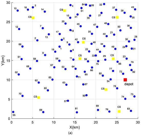
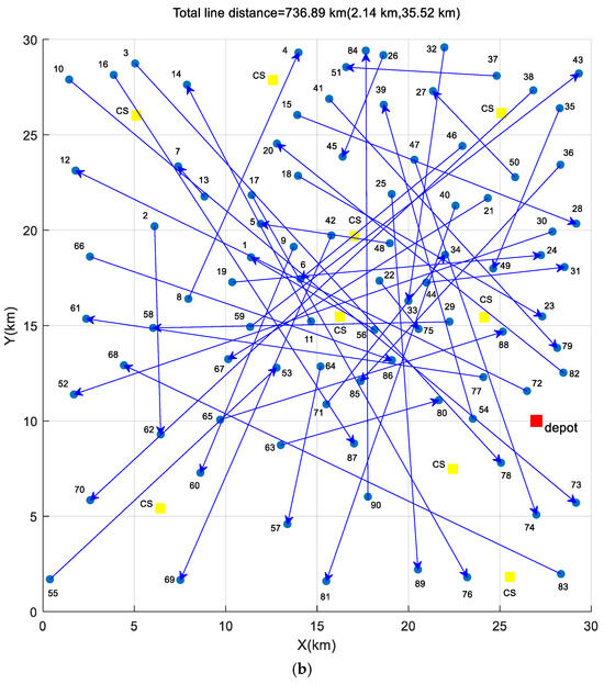
Figure 3. The benchmark testing area with 100 nodes. (a) The node distribution map; (b) the demand graph (The red box represents the depot, the yellow box represents the charging station, the blue dot represents the user node, and the blue arrow represents the user demand arc, pointing from the user’s departure to the destination).

Figure 3a is a node distribution diagram without any arcs. The upper right corner is the urban area of Wuhan with a relatively dense population, while the lower left corner is the suburban area of Wuhan with a relatively sparse population. This figure includes a central depot that provides both recharging and battery-swapping services, as well as nine large charging stations that only offer recharging. A total of 45 user demands were randomly generated in the entire testing area, with each user demand generating a pair of nodes, namely, a departure node and a destination, totaling 90 user nodes. In the figure, 90 blue dots represent user nodes, 9 yellow square dots denote charging stations (marked as CS), and a red square dot is the depot. Therefore, there are a total of 100 charging stations and user nodes.

Figure 3b is a demand graph, where the arc between a pair of nodes represents a user demand. In Figure 3b, the arrow on each arc points from the departure node to the destination for traveling. The arcs were weighted according to the distances between nodes and calculated using their latitude and longitude coordinates. All AVs depart from the depot in a half-charged state to meet all user demands and ultimately return to the depot after providing joint routing optimization. In urban environments, there is a significant difference between Euclidean and actual Manhattan distances or road network distances, but they can all be described as line segments of a certain length. In benchmark testing, our proposed algorithm and other baseline algorithms will be used to test the ability to quickly traverse all demand arcs without paying too much attention to the turns in these demand arcs.

The detailed benchmark parameters are listed in Table 2. The experiments were run on an Intel(R) Core(TM) i5-8250U with UHD Graphics, a 1.80 GHz CPU, 8.00 GB of RAM, and a 64-bit Windows 10 operating system and MATLAB R2021b simulation software.

Table 2. Benchmark parameters.

Benchmark Parameter	Value
${a(a}_x,a_y)$	[−15 km, +15 km]
$T$	12 h
$t_{a,b}^{ddl}$	[10 min, 60 min]
$a_{max}$	100
$v_{max}$	9
$r_i^{travelm}$	50 km/h
$r_i^{charge}$	300 kW
$r_i^{discha}$	3 kW/h
$b_i^{max}$	60 kWh
$b_i^{min}$	9 kWh
$k_c$	9
$k_s$	1

5.2. Test Results of the Proposed Algorithm

For the APC algorithm, the population size is S = 1000, the seeding probability is $p_{seed}=0.2$, the growing probability is $p_{grow}=0.4$, and the fruiting probability is $p_{fruit}=0.7$. Although there are multiple stopping conditions for iterative computation, the algorithm was terminated at a maximum of 1000 iterations to compare all algorithms.

After 1000 iterations, the routes of nine AVs are shown in Figure 4a,b, where different colors indicate different AV routes. Two scenarios were tested: Figure 4a shows the recharging scheme, and Figure 4b shows the hybrid recharging and swapping scheme. There are 100 vertices in each figure, where each vertex represents a user node or a charging station. Edges between these nodes are defined as the paths of AVs, and the arrows on edges indicate the travel directions.

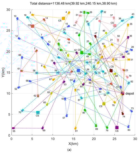
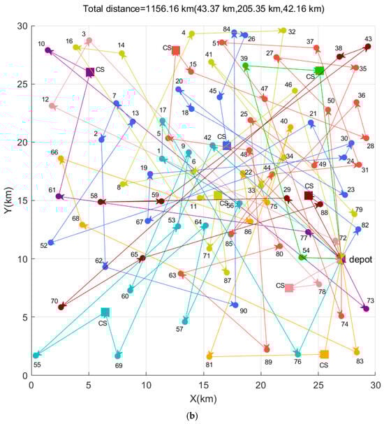
Figure 4. The benchmark testing area with 100 nodes. (a) The charging scheme; (b) the hybrid recharging and swapping scheme (The red box represents the depot, other colored boxes represent charging stations, dots represent user nodes, and different colored directed arcs represent the trajectories of different autonomous vehicles).

In Figure 4a, there are nine charging stations, and the depot can only provide recharging; thus, the APC algorithm employed Algorithm 1 to search for the optimal routes in order to provide the recharging scheme and demand services. We can observe that Figure 4a contains all the arcs in Figure 3b, which respond to all user demands. This scheme exhibits the shortest total distance of 1136.48 km, where the shortest total mileage of a single AV is 39.92 km, and the longest total mileage of a single AV is 240.15 km. In Figure 4b, the depot can provide both recharging and battery-swapping services; therefore, the APC algorithm used Algorithm 2 to provide the hybrid recharging and swapping scheme for demand services. As observed, Figure 4a links all arcs in Figure 3b, which means that all user demands are addressed. This scheme exhibits the shortest total distance of 1156.16 km, where the shortest total mileage of a single AV is 43.37 km, and the longest total mileage of a single AV is 205.35 km. Therefore, the total distance of the hybrid scheme is higher than that of the recharging scheme, and the shortest total distance may increase if the battery-swapping station is located farther away. Therefore, the hybrid scheme will consume more idling time.

Furthermore, the sensitivity of the three parameters of the APC was tested, including the seeding probability $p_{seed}$, growing probability $p_{grow}$, and fruiting probability $p_{fruit}$. Figure 5 illustrates the performance comparison as the seeding probability $p_{seed}$ in the hybrid recharging and swapping scheme increases from 0.1 to 0.9. The performance comparison is conducted with a fixed growing probability $p_{grow}=0.4$ and fixed fruiting probability $p_{fruit}=0.7$. In the seeding operation, a larger seeding probability $p_{seed}$ helps generate more random solutions to improve the global search capability of the APC algorithm. Thus, it is easier to search for the global optimal solution to lower the idling time and charging waiting time. Figure 5 shows that the proposed APC algorithm is still efficient, but the hybrid scheme still consumes more idling time because the battery-swapping station is located farther away.

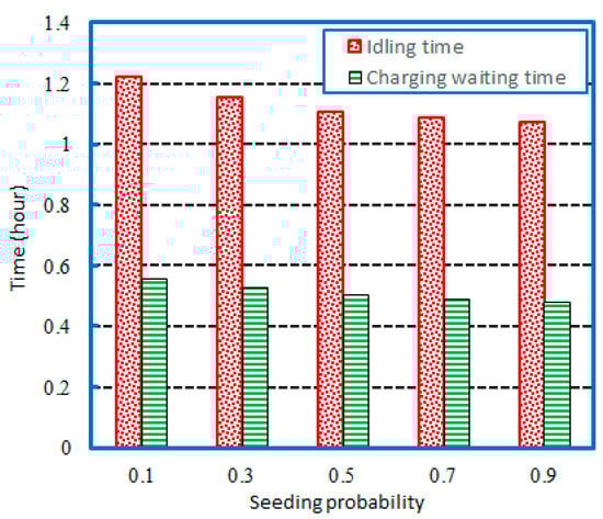
Figure 5. Performance comparison for increasing seeding probability $p_{seed}$.

Figure 6 illustrates the performance comparison as the growing probability $p_{grow}$ in the hybrid recharging and swapping scheme increases from 0.1 to 0.9. The performance comparison is conducted with a fixed seeding probability of $p_{seed}=0.2$ and a fixed fruiting probability of $p_{fruit}=0.7$. In the growing operation, a smaller growing probability $p_{grow}$ helps eliminate more solutions, thereby enhancing the convergence capability of the APC algorithm. As the growing probability $p_{grow}$ increases, it is easier to retain more solutions and prevent premature convergence to local optima, but this comes at the cost of greater computational overhead. Although the population size has increased, the improved growing operation still ensures the convergence ability of the APC algorithm.

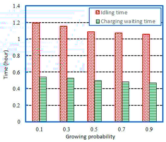
Figure 6. Performance comparison for increasing growing probability $p_{grow}$.

Figure 7 shows the performance comparison for the fruiting probability $p_{fruit}$ in the recharging scheme, which ranges from 0.1 to 0.9. The performance comparison is conducted with a seeding probability of $p_{seed}=0.2$ and a fixed growing probability of $p_{grow}=0.4$. In the fruiting operation, a lower fruiting probability $p_{fruit}$ can increase the cross-learning capability to enhance the local search. Overall, as the fruiting probability $p_{fruit}$ increases, the algorithm is more likely to become trapped in local optima, resulting in higher idling times and charging wait times.

Figure 7. Performance comparison for increasing fruiting probability $p_{fruit}$.

As shown in Figure 4, Figure 5, Figure 6 and Figure 7, the proposed APC algorithm demonstrates efficiency in the two schemes. Among the three parameters of APC, a larger seeding probability $p_{seed}$ is easier to reduce the idling time of AVs by up to 12.357% and the charging waiting time by up to 14.465% in the hybrid recharging and swapping scheme. Hence, the performance advantage of the proposed APC algorithm becomes even more pronounced as the seeding probability $p_{seed}$ increases, where more APC individuals are produced. Although the impact of the growing probability $p_{grow}$ on the global search ability of the APC algorithm is not as significant as that of the seeding probability $p_{seed}$, a smaller growing probability $p_{grow}$ can help accelerate the calculation speed of the APC. The impact of the fruiting probability $p_{fruit}$ on the performance of the APC algorithm is not as significant as the first two parameters, but it can enhance the local search ability and fine tune the optimal solution of the APC algorithm. These findings underscore the clear superiority of the proposed APC algorithm over other methods.

5.3. Algorithm Comparison

For this comparison, some main baseline algorithms were employed for comparative experiments, including the GA [10,24], PSO [12,28], DRL [13,17,33], and ACO [23]. It was assumed that all AVs in the system had identical specifications, as detailed in Section 4.1. For ease of analysis, all comparative experiments were based on the recharging scheme, as the frequency of AV battery swapping was not as high. A maximum of 1000 iterations was used to terminate and compare all algorithms.

For fair testing and comparison, all algorithms used the same population size and basic version. For the GA [10,24], the population size was S = 1000, the chromosome length was Lind = 20, the crossover probability was px = 0.7, and the mutation probability was pm = 0.01. In the PSO [12,28], we set the population size to S = 1000, the location limitation to 0.5, the speed limitation to [−0.5, 0.5], the self-learning factor to c1 = 1.5, and the social learning factor to c2 = 1.5. In the DRL [13,17,33], we set a state embedding network, including a shared stack and multiple heads, and the output from the shared stack was directed towards the head blocks, where each block contained 100 ReLU units followed by |V| + 1 units with tanh activation. The shared stack encompassed two hidden layers, with a batch normalization layer sandwiched between them, where each hidden layer comprised 200 neurons activated by the ReLU function. The option embedding network mirrored the architecture of the aforementioned shared stack, with the exception that each hidden layer utilized 100 ReLU units. The tanh function was selected due to its zero-centered nature and its output range being confined between −1 and 1. The parameters of ACO [23] are as follows: population size of S = 1000 ants; importance of heuristic factors = 5.0; pheromone volatilization factor = 0.1; and pheromone importance = 1.0.

First, we compared the solution results of different algorithms when the number of user nodes changed, including the average idling time in Figure 8 and the average charging waiting time in Figure 9. The total number of user nodes for AVs ranged from 100 to 500 over a 12 h scheduling period, encompassing a mix of short and long travel with random distributions. The number of charging stations was fixed at 10.

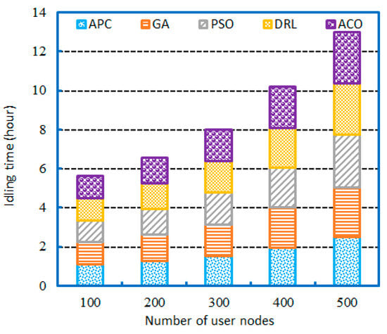
Figure 8. Comparison of the average idling time for increasing the number of user nodes.

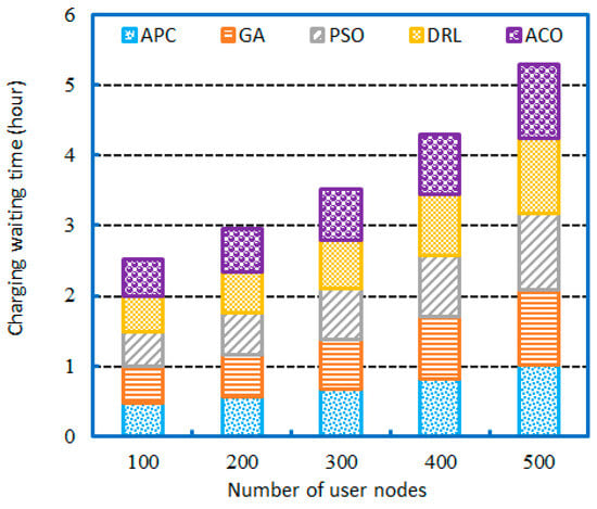
Figure 9. Comparison of the average charging waiting time for increasing the number of user nodes.

Figure 8 shows the comparison of the average idling time for increasing the number of user nodes, ranging from 100 to 500. Figure 8 increases the scale of the problem and the difficulty of the solution to satisfy all user demands across the main baseline algorithms. Starting with a scenario of 100 demands, the APC required an average of 1.101 h of idling time, while the ACO required 1.126 h of idling time. However, as the number of user nodes increased, it lengthened the shortest paths. The efficiency of the APC remained consistent even as the number of demands increased, constantly meeting the demands with the lowest average idling time among the six approaches. For instance, with 500 demands, the APC algorithm required 2.519 h of average idling time, and the PSO required 2.693 h, with a maximum improvement of 6.908%.

These findings indicate that the APC consistently searches for a lower average idling time through enhanced global and local search capabilities. When the number of user nodes increases, compared with other baseline algorithms, the proposed APC algorithm can more efficiently run two strategies, i.e., the recharging scheme and hybrid recharging and swapping scheme, to optimize demand services.

Figure 9 presents a comparison of the average charging waiting time as the number of user nodes increases from 100 to 500. All AVs were assumed to be identical, and the number of charging stations at each station was taken from the dataset in Section 4.1. Using the same geographical data for charging stations in Wuhan, the proposed APC algorithm has significant advantages over the other five baseline approaches based on the average charging waiting time. We began with 100 user nodes, where the APC saved 0.02655 h of charging waiting time compared with the GA. As the number of user nodes increased, the driving range of the AVs also increased. With 500 user nodes, the APC’s savings grew to 0.0817 h of charging waiting time compared with the PSO, achieving up to 8.053% in improvement. Figure 9 illustrates the charging waiting time as the number of user nodes varies, clearly showing that the APC performs better in scenarios with more user demands.

Second, we compared the solution results of different algorithms when the number of charging stations changed, including the average idling time shown in Figure 10 and the average charging waiting time shown in Figure 11. The total number of charging stations for AVs ranged from 10 to 50 over a 12 h scheduling period, encompassing a mixture of short and long travel with random distributions. The number of user nodes was fixed at 100.

Figure 10. Comparison of the average idling time for increasing the number of charging stations.

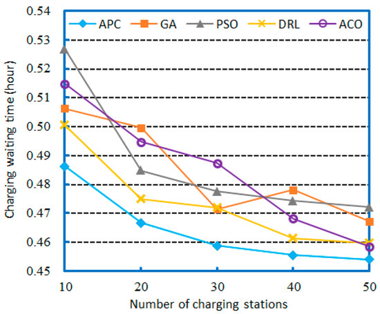
Figure 11. Comparison of the average charging waiting time with an increase in the number of charging stations.

Figure 10 illustrates the comparison of the average idling time for increasing the number of charging stations, ranging from 10 to 50. Clearly, with the increase in charging facilities, the idling time in both scenarios can be greatly reduced. This reduction is primarily because more charging stations result in shorter charging waiting times for AVs, allowing each vehicle to be utilized for longer periods and distances for demand services while adhering to the required deadlines. A similar trend is depicted in Figure 10, which shows the comparison of the six approaches regarding the search performance. For 10 charging stations, the APC saves 0.0804 h of idling time compared with the ACO. Similarly, for 50 charging stations, the APC achieved a total saving of 0.0423 h compared with the ACO. Hence, the APC performs more efficiently, achieving up to 7.302% improvement in the average idling time, which is lower than other baseline algorithms.

Figure 11 displays a comparison of the average charging waiting time as the number of charging stations increases from 10 to 50. In this experiment, we fixed the number of demands at 100 using the demand graph derived from the dataset in Section 4.1. No AV could traverse more than one node on a full battery charge. When the number of charging stations was set to 10, the APC outperformed the other methods, saving 0.04045 h of the charging waiting time compared with the PSO, with a maximum improvement of 8.319%. As the number of charging stations increased to 50, the APC achieved substantial savings, reducing the average charging waiting time by 0.0181 h compared with GA. Figure 11 illustrates the negative relationship between the number of charging stations and the average charging waiting time. The findings suggest that more charging stations shorten the distance between the departure node and the destination, and the APC efficiently selects the shortest route, often fulfilling the demand without requiring additional charging waiting time.

We performed at least 10 identical tasks, executed at least 500 iterations, and conducted statistical tests. Statistical testing included three scenarios—namely, Scenario 1, where the number of user nodes is 100 and the number of charging stations is 10, Scenario 2, where the number of user nodes is 100 and the number of charging stations is 50, and Scenario 3, where the number of user nodes is 500 and the number of charging stations is 10. In each scenario, we provide the idling time ${\sum }_i{t}_i^{idl}$, charging waiting time ${\sum }_i{t}_i^{waitc}$, and computation time as comparison metrics. The statistical data are shown in Table 3, including the maximum, minimum, and average values; the upper limit of (95% CI/UL) and the lower limit of (95% CI/LL) of the 95% confidence interval; and the execution time of each method.

Table 3. Statistical data.

Metrics		APC	GA	PSO	DRL	ACO
Scenario 1:	computation time (minutes)	13.43	14.59	15.26	64.81	15.92
${\sum }_i{t}_i^{idl}$	max	1.162	1.228	1.213	1.186	1.217
	min	1.064	1.128	1.118	1.089	1.114
	avg	1.109	1.158	1.153	1.128	1.163
	95% CI/UL	1.120	1.172	1.164	1.139	1.176
	95% CI/LL	1.098	1.145	1.142	1.117	1.151
	variance	0.00064	0.00094	0.00063	0.00066	0.00078
${\sum }_i{t}_i^{waitc}$	max	0.548	0.569	0.577	0.538	0.545
	min	0.505	0.540	0.547	0.503	0.509
	avg	0.521	0.543	0.548	0.512	0.523
	95% CI/UL	0.527	0.547	0.553	0.517	0.526
	95% CI/LL	0.515	0.539	0.543	0.508	0.519
	variance	0.00017	0.00008	0.00013	0.00010	0.00008
Scenario 2:	computation time (minutes)	13.51	14.74	15.63	65.38	16.17
${\sum }_i{t}_i^{idl}$	max	1.134	1.159	1.148	1.132	1.194
	min	1.030	1.046	1.055	1.033	1.083
	avg	1.051	1.118	1.091	1.075	1.107
	95% CI/UL	1.068	1.134	1.102	1.086	1.125
	95% CI/LL	1.034	1.102	1.081	1.063	1.088
	variance	0.00149	0.00130	0.00058	0.00069	0.00185
${\sum }_i{t}_i^{waitc}$	max	0.497	0.529	0.548	0.493	0.532
	min	0.452	0.481	0.493	0.465	0.490
	avg	0.464	0.490	0.512	0.472	0.503
	95% CI/UL	0.471	0.499	0.521	0.475	0.509
	95% CI/LL	0.457	0.481	0.502	0.469	0.497
	variance	0.00027	0.00044	0.00050	0.00005	0.00017
Scenario 3:	computation time (minutes)	13.64	14.95	16.17	65.98	16.46
${\sum }_i{t}_i^{idl}$	max	2.570	2.635	2.841	2.711	2.673
	min	2.477	2.535	2.684	2.616	2.572
	avg	2.520	2.578	2.756	2.656	2.612
	95% CI/UL	2.530	2.590	2.784	2.667	2.624
	95% CI/LL	2.510	2.566	2.727	2.645	2.600
	variance	0.00052	0.00069	0.00424	0.00060	0.00079
${\sum }_i{t}_i^{waitc}$	max	1.045	1.130	1.152	1.112	1.100
	min	1.010	1.078	1.099	1.081	1.044
	avg	1.020	1.094	1.119	1.083	1.063
	95% CI/UL	1.024	1.103	1.128	1.088	1.073
	95% CI/LL	1.016	1.085	1.111	1.078	1.053
	variance	0.00009	0.00042	0.00038	0.00013	0.00051

Table 3 shows that the proposed APC algorithm had significant improvements compared to other baseline algorithms, with a maximum improvement of 10.512% at the maximum idling time ${\sum }_i{t}_i^{idl}$ in Scenario 3 and 10.290% at the average charging waiting time ${\sum }_i{t}_i^{waitc}$ in Scenario 2.

5.4. Discussion

In summary, the above comparative experiments, as shown in Figure 5, Figure 6, Figure 7, Figure 8, Figure 9, Figure 10 and Figure 11 and Table 3, compare the performance of the proposed APC algorithm and other baseline methods in minimizing the idling and charging waiting times required under varying deadlines. All six algorithms yielded similar trends, as reflected in Figure 5, Figure 6, Figure 7, Figure 8, Figure 9, Figure 10 and Figure 11 and Table 3. However, as the number of user nodes increased, both the idling time and the charging waiting time began to show significant improvements, and the APC demonstrated effectiveness and showed significant advantages in saving time compared with other baseline algorithms. As the number of charging stations increased, both the idling time and the charging waiting time began to present a downward trend. This analysis suggests that more charging stations can help save time, but the APC can achieve cost savings by reasonably arranging the AVs to meet the demands.

It is worth mentioning that the DRL [13,17,33] algorithm has also demonstrated strong problem-solving ability and can provide high-precision solutions, but it requires lengthy offline training. The proposed APC algorithm still has advantages because it only requires real-time iterative optimization, whereas DRL should be evaluated based on its inference time.

In Equation (1) of Section 3.1, the distance between two nodes is defined as the Euclidean distance. Our simplified experimental roadmap may not be consistent with the actual situation, which may result in a planned “optimal path” that is completely unfeasible in reality (for example, directly passing through buildings or rivers).

However, our technical solution is based on the five basic assumptions provided in Section 3.2. Although it simplifies the analysis, it also ignores some practical factors, such as the extremely complex process of battery aging and degradation after multiple recharges [18]. Moreover, a fast recharging rate may accelerate battery aging and degradation, but the underlying mechanisms need further investigation.

Additionally, the battery-swapping time was set as zero in this study. In most cases, the battery-swapping speed is much faster than the recharging speed, and this assumption also applies. However, with the rapid development of fast recharging technology and the improvement of battery performance, there may be a situation in the future where the recharging rate and battery exchange rate are comparable, which needs to be analyzed in subsequent research.

6. Conclusions

AVs are a product of the combination of advances in vehicle technology and artificial intelligence, but they face challenges with respect to recharging and battery swapping. This study addressed the joint routing optimization problem of AVs under recharging and battery-swapping modes. Unlike much of the existing literature, our system was modeled as a demand graph, and the goal of our work was to meet all user demand arcs within these deadlines while minimizing multi-objectives, i.e., the total distance, idling time, and charging waiting time of the AVs. Given the NP-hard nature of this problem, an improved APC algorithm was proposed as a solution. The seeding, growing, and fruiting operations of the proposed APC algorithm were enhanced to improve its search capability. A benchmark test set was developed based on the road environment in Wuhan, China, and our test dataset conformed to the non-uniform population distribution in Wuhan. The experimental results revealed that the proposed APC algorithm has significant improvements compared to other baseline algorithms, with a maximum improvement of 10.512% at the maximum idling time ${\sum }_i{t}_i^{idl}$ and 10.290% at the average charging waiting time ${\sum }_i{t}_i^{waitc}$.

Due to experimental limitations, the main shortcoming of this study is that it was simulated on a PC rather than deployed on a real AV platform; hence, some practical factors may have been overlooked. The impact of a fast-charging operation on battery aging and degradation is extremely complex, and its mechanism of influence was beyond the scope of this manuscript. In addition, the battery-swapping time was assumed to be zero, which requires further research. In future studies, we plan to deploy the algorithm on a real edge computing platform and incorporate additional factors, such as actual Manhattan or road network distances; fairer algorithm comparisons; and the memory usage, power consumption, and actual reasoning delay of low-computing-power devices.

References

- Miller, T.; Durlik, I.; Kostecka, E.; Borkowski, P.; Lobodzinska, A. A critical AI view on autonomous vehicle navigation: The growing danger. Electronics 2024, 13, 3660. [Google Scholar] [CrossRef]
- Gao, J.; Li, S. Charging autonomous electric vehicle fleet for mobility-on-demand services: Plug in or swap out? Transp. Res. Part C Emerg. Technol. 2024, 158, 104457. [Google Scholar] [CrossRef]
- Han, Y.-J.; Kim, B.-C.; Xu, H.-C. Deep learning-based trajectory tracking method for intelligently network-connected driverless vehicles in narrow areas. Inf. Technol. Control 2024, 53, 1221–1235. [Google Scholar] [CrossRef]
- Xia, T.; Chen, H. A survey of autonomous vehicle behaviors: Trajectory planning algorithms, sensed collision risks, and user expectations. Sensors 2024, 24, 4808. [Google Scholar] [CrossRef] [PubMed]
- Ma, B.; Hu, D.; Wang, Y.; Sun, Q.; He, L.; Chen, X. Time-dependent vehicle routing problem with departure time and speed optimization for shared autonomous electric vehicle service. Appl. Math. Model. 2023, 113, 333–357. [Google Scholar] [CrossRef]
- Huang, A.; Zhang, Y.; He, Z.; Hua, G.; Shi, X. Recharging and transportation scheduling for electric vehicle battery under the swapping mode. Adv. Prod. Eng. Manag. 2021, 16, 359–371. [Google Scholar] [CrossRef]
- Zhang, Z. Exploring rounD dataset for domain generalization in autonomous vehicle trajectory prediction. Sensors 2024, 24, 7538. [Google Scholar] [CrossRef] [PubMed]
- Wang, S.; Lin, F.; Wang, T.; Zhao, Y.; Zang, L.; Deng, Y. Autonomous vehicle path planning based on driver characteristics identification and improved artificial potential field. Actuators 2022, 11, 52. [Google Scholar] [CrossRef]
- Saha, P.K.; Chakraborty, N.; Mondal, A.; Mondal, S. Optimal sizing and efficient routing of electric vehicles for a vehicle-on-demand system. IEEE Trans. Ind. Inform. 2022, 18, 1489–1499. [Google Scholar] [CrossRef]
- Chu, K.-F.; Lam, A.Y.S.; Li, V.O.K. Joint rebalancing and vehicle-to-grid coordination for autonomous vehicle public transportation system. IEEE Trans. Intell. Transp. Syst. 2022, 23, 7156–7169. [Google Scholar] [CrossRef]
- Xu, Y.; Yang, J.; Lai, K.; Xu, Y.; Zhang, M. Joint distribution route optimization of fresh supplies by electric vehicles under charging and battery-swapping modes. Adv. Mech. Eng. 2025, 17, 16878132251348353. [Google Scholar] [CrossRef]
- Abo-Elyousr, F.K.; Sharaf, A.M.; Lehtonen, M.; Darwish, M.M.F.; Mahmoud, K. Optimal scheduling of DG and EV parking lots simultaneously with demand response based on self-adjusted PSO and K-means clustering. Energy Sci. Eng. 2022, 10, 4025–4043. [Google Scholar] [CrossRef]
- Che, A.; Wang, Z.; Zhou, C. Multi-agent deep reinforcement learning for recharging-considered vehicle scheduling problem in container terminals. IEEE Trans. Intell. Transp. Syst. 2024, 25, 16855–16868. [Google Scholar] [CrossRef]
- Wang, D.; Xu, H.; Guo, J.; Dai, L.; Zhang, L. Optimizing highway electric vehicle scheduling and battery swapping station management for enhanced renewable energy utilization. Electronics 2025, 14, 952. [Google Scholar] [CrossRef]
- Cai, Z.; Jiang, S.; Dong, J.; Tang, S. An artificial plant community algorithm for the accurate range-free positioning of wireless sensor networks. Sensors 2023, 23, 2804. [Google Scholar] [CrossRef]
- Zhang, S.; Tang, Z.; Li, L. Electric vehicle routing problem with pickup and delivery under the partial recharging and nonlinear discharging strategy. Int. J. Shipp. Transp. Logist. 2025, 20, 407–436. [Google Scholar] [CrossRef]
- Liang, Y.-C.; Ding, Z.-H.; Ding, T.; Lee, W.-J. Mobility-aware charging scheduling for shared on-demand electric vehicle fleet using deep reinforcement learning. IEEE Trans. Smart Grid 2021, 12, 1380–1393. [Google Scholar] [CrossRef]
- Xu, M.; Wu, T.; Tan, Z.-J. Electric vehicle fleet size for car sharing services considering on-demand charging strategy and battery degradation. Transp. Res. Part C Emerg. Technol. 2021, 127, 103146. [Google Scholar] [CrossRef]
- Dean, M.D.; Gurumurthy, K.M.; de Souza, F.; Auld, J.; Kockelman, K.M. Synergies between repositioning and charging strategies for shared autonomous electric vehicle fleets. Transp. Res. Part D Transp. Environ. 2022, 108, 103314. [Google Scholar] [CrossRef]
- Ammous, M.; Belakaria, S.; Sorour, S.; Abdel-Rahim, A. Joint delay and cost optimization of in-route charging for on-demand electric vehicles. IEEE Trans. Intell. Veh. 2020, 5, 149–164. [Google Scholar] [CrossRef]
- Lian, Y.; Lucas, F.; Sörensen, K. The electric on-demand bus routing problem with partial charging and nonlinear function. Transp. Res. Part C Emerg. Technol. 2023, 157, 104368. [Google Scholar] [CrossRef]
- Nafstad, G.M.; Desaulniers, G.; Stålhane, M. Branch-price-and-cut for the electric vehicle routing problem with heterogeneous recharging technologies and nonlinear recharging functions. Transp. Sci. 2025, 59, 628–646. [Google Scholar] [CrossRef]
- Comert, S.E.; Yazgan, H.R. A new approach based on hybrid ant colony optimization-artificial bee colony algorithm for multi-objective electric vehicle routing problems. Eng. Appl. Artif. Intell. 2023, 123, 106375. [Google Scholar] [CrossRef]
- Londoño, A.A.; Gonzalez, W.G.; Giraldo, O.D.M.; Escobar, J.W. A new matheheuristic approach based on Chu-Beasley genetic approach for the multi-depot electric vehicle routing problem. Int. J. Ind. Eng. Comput. 2023, 14, 555–570. [Google Scholar] [CrossRef]
- Çatay, B.; Sadati, I. A note on battery swapping policies in the electric vehicle routing problem with time windows and battery swapping vehicles. Comput. Oper. Res. 2025, 185, 107277. [Google Scholar] [CrossRef]
- Zhang, T.; Peng, Q.; Zeng, S. Predicting EV charging demand in renewable-energy-powered grids using explainable machine learning. Sustainability 2025, 17, 4158. [Google Scholar] [CrossRef]
- Wang, X.-L.; Zhang, Z.-Y.; Jiang, M.-M.; Wang, Y.-F.; Wang, Y.-P. Scheduling model and algorithm for transportation and vehicle charging of multiple autonomous electric vehicles. Mathematics 2025, 13, 145. [Google Scholar] [CrossRef]
- Shaheen, H.I.; Rashed, G.I.; Yang, B.; Yang, J. Optimal electric vehicle charging and discharging scheduling using metaheuristic algorithms: V2G approach for cost reduction and grid support. J. Energy Storage 2024, 90, 111816. [Google Scholar] [CrossRef]
- Cai, Z.-Y.; Wang, X.-L.; Li, R.; Gao, Q. An artificial physarum polycephalum colony for the electric location-routing problem. Sustainability 2023, 15, 16196. [Google Scholar] [CrossRef]
- Cai, Z.; Yu, Q.; Lu, Z.; Liu, Z.; Gong, G. An artificial plant community algorithm for collision-free multi-robot aggregation. Appl. Sci. 2025, 15, 4240. [Google Scholar] [CrossRef]
- Hu, X.; Zhang, Z.; Fan, Z.; Yang, J.; Yang, J.; Li, S.; He, X. GCN-transformer-based spatio-temporal load forecasting for EV battery swapping stations under differential couplings. Electronics 2024, 13, 3401. [Google Scholar] [CrossRef]
- Qu, H.-H.; Kuang, H.-X.; Wang, Q.-X.; Li, J.; You, L.-L. A physics-informed and attention-based graph learning approach for regional electric vehicle charging demand prediction. IEEE Trans. Intell. Transp. Syst. 2024, 25, 14284–14297. [Google Scholar] [CrossRef]
- Ji, Y.; Huang, Y.; Yang, M.; Leng, H.; Ren, L.; Liu, H.; Chen, Y. Physics-informed deep learning for virtual rail train trajectory following control. Reliab. Eng. Syst. Saf. 2025, 261, 111092. [Google Scholar] [CrossRef]
Disclaimer/Publisher’s Note: The statements, opinions and data contained in all publications are solely those of the individual author(s) and contributor(s) and not of MDPI and/or the editor(s). MDPI and/or the editor(s) disclaim responsibility for any injury to people or property resulting from any ideas, methods, instructions or products referred to in the content. |
© 2025 by the authors. Licensee MDPI, Basel, Switzerland. This article is an open access article distributed under the terms and conditions of the Creative Commons Attribution (CC BY) license (https://creativecommons.org/licenses/by/4.0/).