ICEEMDAN- and LSTM-Enhanced Hybrid Cosine-Attention iTransformer for Ultra-Short-Term Load Forecasting

Abstract

Accurate power system load forecasting is the core prerequisite for guaranteeing the safe and stable operation of power grids and supporting the efficient scheduling of power systems. To improve the accuracy of load forecasting and portray the non-stationarity and multi-scale characteristics of the load sequence, this paper proposes a short-term load forecasting method based on ICEEMDAN decomposition-LSTM feature extraction-hybrid cosine attention mechanism iTransformer. Firstly, the original load sequence is decomposed using the Improved Complete Ensemble Empirical Modal Decomposition (ICEEMDAN) to extract the intrinsic modal function (IMF) and residuals (Res), and the multidimensional input feature set is constructed by combining exogenous variables such as meteorology. Secondly, multi-source features were extracted using the Long Short-Term Memory (LSTM) network to capture the complex nonlinear correlations and long-term dependencies. Finally, the extracted features are input into the iTransformer model that introduces the hybrid cosine attention mechanism. The hidden feature representation is obtained through the encoder layer modeling, and the linear mapping in the output layer generates the load forecast value. The results show that the prediction method proposed in this paper achieves better performance and can effectively improve the accuracy of short-term load prediction, which provides an effective technical support for the short-term scheduling and flexible operation of the power system.

1. Introduction

Load forecasting is a key aspect of power system operation and planning, aiming at modeling and analyzing the data of historical loads and related external factors to infer the power demand in future periods [1]. The accuracy of its forecasting directly affects system supply–demand balance, dispatch plan formulation, and the assessment of operating costs and security margins [2,3,4]. Under ultra-short-term scales, the load sequence presents significant stochastic fluctuations and non-stationarity, which makes the forecasting error further amplified in the spare capacity allocation, power market clearing, and demand-side response. Meanwhile, with the diversification of demand-side electricity consumption behaviors, the load series is often superimposed with stochastic, seasonal, and cyclical components, and subject to the combined influence of external factors such as meteorological conditions [5]. Therefore, achieving stable and high-precision load forecasting under complex disturbances and multidimensional coupling conditions has become a core scientific problem and engineering challenge in power system optimal operation and planning [6].

Existing load forecasting technology systems can be classified into three categories: physical mechanism, statistical, and artificial intelligence. Early load forecasting mainly relies on physical mechanism models, which are usually based on physical and engineering principles and are constructed by combining equipment energy consumption feature portrayal and user behavior patterns [7,8]. This type of approach is theoretically highly interpretable, but its applicability in short-term grid scenarios is limited by its cumbersome parameter calibration, high sensitivity to user group heterogeneity, and external environmental perturbations [9]. As a result, research is gradually shifting towards data-driven approaches.

With the expansion of power system data scale, statistical modeling methods have gradually become the mainstream of research, and typical methods include autoregressive moving average (ARIMA) [10] and seasonal autoregressive (SARIMA) [11]. Although statistical models have a clear mathematical foundation and strong interpretability, they can effectively portray the trend and periodicity characteristics in smooth or weakly nonlinear load series [12]. However, electricity load data usually exhibit non-stationarity and random fluctuations, and the prediction accuracy of statistical models significantly decreases when disturbed by extreme weather or holidays [13].

To cope with the limitations of statistical models in representing non-smooth and nonlinear load data, researchers have introduced machine learning methods, including support vector machine (SVM) and random forest (RF). Dong et al. firstly used K-means clustering algorithm to classify weekday and holiday patterns of electricity load data, and then constructed a prediction model by using SVM. The accuracy of short-term forecasting of electricity load was effectively improved [14]. Jiang et al. combined stochastic method, grey box model, and random forest method to forecast flexible loads of split air conditioners, which effectively characterized the energy performance of split air conditioners at both individual and aggregate levels [15]. The above methods enhance the modeling capability through nonlinear mapping and integration strategies and achieve better performance than statistical models in some tasks. However, the machine learning methods mainly rely on feature extraction and windowing modeling when representing long sequences and have limited ability to portray multi-scale dynamic features and long-range dependencies [16,17].

With the development of deep learning, neural network models are widely used for load forecasting. Recurrent Neural Networks (RNN), Long Short-Term Memory Networks (LSTM), and Gated Recurrent Units (GRUs) perform well in capturing time-dependent and nonlinear features [18,19]. Wen et al. proposed an improved recurrent neural network based on recurrent neural network to predict the day-ahead wholesale tariff, photovoltaic (PV) power output, and power load, which achieved better performance [20]. Wan et al. proposed a new method for short-term power load forecasting combining convolutional neural network (CNN), LSTM, and attention mechanism, which solves the problem of information loss due to the excessive length of input time series data [21]. Fan et al. proposed a two-layer GRU network optimized by the Improved Multi-Objective Evolutionary Algorithm (MOEA/D), which was tested in two load forecasting sets, and the proposed model demonstrated good accuracy and generalization [22]. However, although the above models overcome to some extent the limitation of insufficient capture of artificial feature dependencies and long-distance dependencies in terms of long sequence modeling and prediction accuracy, they still face the gradient decay problem when representing long sequences and lack an explicit modeling mechanism for cross-variate dependencies [23].

In this context, the transformer architecture was introduced for time series forecasting due to its parallel modeling capabilities based on the self-attention mechanism [24]. The transformer architecture demonstrates the advantages of parallel modeling and long-range dependency representation in time series forecasting, however, its lack of inductive bias on local time series patterns and limited ability to model cross-feature dependencies in multivariate scenarios constrains its performance in complex load forecasting tasks. Researchers have proposed a variety of improved models in the literature. Zhou et al., proposed the informer model, which reduces complexity and improves prediction efficiency through sparse attention with a hierarchical distillation mechanism [25]. Wu et al., proposed the autoformer model, which embedded decomposition operators into the network structure and introduced autocorrelation mechanisms to enhance the cyclic modeling capability [26]. Zhou et al., proposed the FEDformer model to achieve more efficient multi-scale feature extraction in the framework of frequency and time domain decomposition [27]. These works promoted the development of transformer in time series forecasting from the perspectives of efficiency optimization, cycle-dependent modeling, and multiscale decomposition, respectively, but their common limitation is that they are mainly oriented to long time scale tasks, and they do not sufficiently portray high frequency fluctuations and cross-variate correlations in short-term forecasting [28].

To address the limitations, iTransformer takes variables rather than time-steps as the basic unit of modeling, thus realizing the inverted dimensionality design of variables as tokens [29]. This structure can explicitly portray the interactions between different variables, which significantly enhances the ability to model the dependence on multiple input features, such as the decomposed IMF components, residuals, and meteorological exogenous variables [30]. This method makes up for the shortcomings of the traditional transformer in multivariate time series forecasting, but still fails to adequately capture the local time-series patterns and nonlinear dynamic features. The LSTM network has a natural advantage in modeling short-term dependence and nonlinear dynamics, and its gating mechanism can effectively alleviate the gradient vanishing problem, which makes it suitable for extracting local features of loaded sequences. However, LSTM lacks effective exploitation of cross-feature interactions in multivariate scenarios. Therefore, combining LSTM with iTransformer, where the former is used to capture local nonlinear and short-term dynamic features, and the latter is used to portray cross-feature dependencies and global relationships, can complement each other’s strengths, and provide a more robust modeling framework for predicting complex load sequences.

The combination of LSTM-iTransformer improves the model’s ability to comprehensively model local and global features, but the iTransformer still relies on the standard self-attention mechanism internally, which is prone to the problem of unstable attention distribution in high-dimensional scenarios and the risk of under-utilization of information. For this reason, this paper introduces a hybrid cosine attention mechanism into the framework. This mechanism borrows the idea of cosine kernel from CosFormer, which retains the basis of Softmax, weakens the paradigm difference through cosine normalization, and combines with non-negative constraints to improve the stability and focusing of the attention distribution, to enhance the ability to capture the dependency relationships across time scales and feature dimensions [31].

Short-term load series usually show strong volatility and complex non-stationary features, which will reduce the prediction accuracy if directly used for modeling, so it is necessary to pre-process the data by empirical mode decomposition-like methods [32]. Currently, commonly decomposition methods include ensemble empirical mode decomposition (EEMD), complete ensemble empirical mode decomposition with adaptive noise (CEEMDAN), and variational mode decomposition (VMD), among others [33,34,35]. These methods can alleviate the complexity of non-stationary signals to a certain extent, but there are still problems such as mode mixing, inaccurate estimation of instantaneous frequency or insufficient portrayal of local characteristics, which may lead to pseudo-modal decompositions or omission of key information in the decomposition results. In contrast, the improved complete ensemble empirical mode decomposition with adaptive noise (ICEEMDAN) effectively overcomes the shortcomings of the traditional method by introducing adaptive noise in the iterative process and adopting the ensemble averaging strategy. ICEEMDAN effectively overcomes the shortcomings of traditional methods by introducing adaptive noise in the iterative process and adopting an ensemble averaging strategy and can obtain more robust and physically clearer intrinsic mode function components [36]. In this paper, ICEEMDAN is used as a preprocessing tool to decompose the load sequence at multiple scales and construct the input feature set by combining the meteorological variables, to provide a clearer and hierarchical feature support for the LSTM—iTransformer model.

Short-term load series exhibit pronounced volatility and strong non-stationarity, while existing decomposition–transformer hybrid models still suffer from notable limitations in utilizing multi-scale components and modeling cross-variable dependencies. First, the decomposed IMF components are typically treated as static inputs, lacking explicit characterization of their internal local dynamics and fast fluctuations. Second, the decomposition results and deep models are often combined in a simple cascaded manner, without establishing a coherent mechanism that integrates multi-scale components, local temporal structures, and global cross-variable dependencies. Third, the standard scaled dot-product attention is sensitive to magnitude and unit discrepancies, which easily induces attention bias in multivariate settings and thereby weakens the representation of complex coupled relationships. Therefore, this study proposes a hybrid forecasting framework based on ICEEMDAN–LSTM–iTransformer-hybrid cosine attention forecasting model to enhance the accuracy and robustness of short-term load forecasting. The main contributions of this work are as follows:

• The Improved Complete Ensemble Empirical Modal Decomposition (ICEEMDAN) was introduced to solve the problems of modal aliasing and instantaneous frequency estimation bias that are commonly found in traditional decomposition methods. By decomposing the original load sequence into intrinsic modal functions (IMFs) and residuals with different scale characteristics and fusing them with exogenous variables such as meteorology, a clearer and more hierarchical input feature set is constructed, which provides a solid feature base for the subsequent deep model.
• The LSTM and iTransformer architectures were combined. The former can effectively capture short-term dependencies and nonlinear dynamics to alleviate the problem of gradient vanishing; the latter adopts a variable-as-token representation for multi-source inputs, explicitly capturing cross-variable dependencies and global relationships. The two models complement each other and overcome the inadequacy of a single model in modeling local dynamics or global interactions.
• The hybrid cosine attention mechanism was incorporated based on iTransformer and draw on the idea of CosFormer to introduce cosine reweighting and non-negative constraints, improve the numerical stability of the distribution of the attention, enhance the focusing of the weights, and reduce the computational complexity in high-dimensional scenarios. The mechanism enables the model to portray the dynamic dependence of loads more effectively on different time scales and capture the interaction between multi-source features.

The rest of this paper is structured as follows: Section 2 introduces the overall framework of the proposed method and describes the principle and implementation of ICEEMDAN decomposition, LSTM feature extraction, iTransformer global modeling and hybrid cosine attention mechanism. Section 3 gives the construction process of the complete model and details of the algorithms. Section 4 describes the source of the experimental data, the pre-processing method and the evaluation index. Section 5 verifies and analyses the effectiveness of the proposed method through comparative experiments and ablation experiments. Section 6 concludes the whole paper and discusses future research.

2. Model Construction

The ICEEMDAN–LSTM–iTransformer-hybrid cosine attention forecasting framework proposed in this study is illustrated in Figure 1. It introduces a structural advancement over existing approaches. ICEEMDAN employs adaptive-noise decomposition to obtain multi-scale IMFs, enabling an explicit separation between high-frequency fluctuations and low-frequency trends. LSTM further encodes the local dynamics and short-term perturbations within each IMF, providing the short-window memory structure required for ultra-short-term forecasting. The iTransformer models cross-variable dependencies in a variable-as-token manner, addressing the limitations of conventional transformers in representing variable interactions. Moreover, the hybrid cosine attention mechanism mitigates the norm sensitivity of standard scaled dot-product attention by applying directional normalization and gated reweighting, thereby stabilizing the attention distribution under noisy and highly volatile conditions. Through clear functional division and tight cooperation among these components, the proposed framework is capable of simultaneously handling non-stationarity, multi-scale characteristics, high-frequency disturbances, and cross-variable coupling—key challenges intrinsic to ultra-short-term load forecasting.

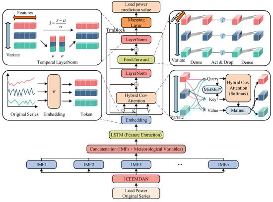
Figure 1. Hybrid forecasting framework. The sign * denotes the cosine normalization of Q, K before MatMul. Hybrid Cos-Attention (Softmax) denotes the attention matrix obtained by Softmax normalization based on normalized similarity, combined with temperature scaling, gated reweighting, and masking operations.

(1)

ICEEMDAN decomposition and feature construction

The raw load series was first decomposed by ICEEMDAN into multiple IMF components together with a residual component (Res). All components were temporally aligned with meteorological variables and concatenated column-wise to form the feature matrix (X_raw) with a structure of [T, C]. To ensure consistent feature scales, the model applied normalization to X_raw using statistics computed from the training segment, producing X_norm. A sliding window of length L was then constructed along the temporal axis, where X_norm[t − L + 1:t] was extracted as the input window (X_win) with dimension [L, C], and the corresponding load value was used as the prediction target (y_target). All samples were partitioned into training, validation, and test sets in chronological order, generating a unified sequential-learning data flow that provided format-consistent inputs for all subsequent model modules.

(2)

LSTM feature extraction

The mini-batch input X_batch has an initial shape of [B, L, C]. The model first transposed this tensor to [B, C, L] so that each variable formed an individual time series of length L within the window. The batch and variable dimensions were then flattened to construct X_seq with shape [B*C, L, 1], where each sequence was encoded by a shared-parameter LSTM. The LSTM recursively propagated its internal states along the temporal dimension and output the final hidden state (h_last) for each sequence, resulting in a representation of size [B*C, d_model]. These states were reshaped back along the variable axis to form the variable-level representation Z with shape [B, C, d_model]. Each vector in Z corresponded to the temporal embedding of one variable within the current window and served as the input unit for cross-variable modeling in the iTransformer.

(3)

iTransformer global dependency modeling

The variable-level representation Z was then fed into the iTransformer encoder to construct global dependency structures along the variable dimension. Each encoder layer first applied layer normalization to the input, followed by linear projections that generated the query Q, key K, and value V matrices, which were rearranged into a multi-head format of shape [B, num_heads, C, head_dim]. The attention operation was performed over the variable dimension so that each variable token updated its representation based on the dynamic embeddings of all other variables. The concatenated multi-head output was linearly projected back to [B, C, d_model], passed through a residual connection and a feed-forward network, and formed the layer output H_block. After stacking multiple layers, the encoder produced H_glob, which remained in shape [B, C, d_model] but encoded global interactions and cross-variable dependencies among all variables.

(4)

Hybrid cosine attention mechanism

Within the attention computation, the model applied directional normalization to Q and K along their last dimension, producing Q_norm and K_norm, so that similarity was dominated by vector direction. The normalized similarity was then scaled by a temperature parameter τ to obtain a controllable similarity response. Meanwhile, K was passed through a linear transformation to generate gate_raw, which was converted to a positive value (gate_pos) via a Softplus operation and further transformed into gate_bias through a logarithmic mapping. This bias term was added to the cosine similarity to modulate variable-wise attention weights, enabling the model to dynamically adjust each variable’s relative contribution based on its characteristics. The final attention matrix (attn) was obtained by Softmax normalization and was used to compute the weighted sum with V, producing the output of each head. All attention heads were concatenated along the head_dim dimension and linearly projected back to the d_model space, completing the mixed cosine-attention representation.

(5)

Predicted output

The global representation (H_glob) produced by the encoder was compressed along the variable dimension through average pooling to obtain h_pool, which has the structure [B, d_model]. This vector integrated both the local temporal features within the window and the cross-variable dependency patterns. The pooled representation (h_pool) was then linearly projected to the prediction dimension, yielding the output y_hat with shape [B, horizon]. During training, the model minimized the mean squared error between the predictions and targets in the normalized space. During inference, y_hat was denormalized and used to compute MAE, RMSE, MAPE, and R² to evaluate predictive performance in the physical scale. This output design ensured that the model leveraged a unified high-dimensional representation to support accurate ultra-short-term load forecasting.

The pseudocode of the algorithm is as follows (Algorithm 1):

Algorithm 1. ICEEMDAN–LSTM–iTransformer with hybrid cosine attention.

Input: multivariate series X ∈ $ℝ$^{T × C} (IMFs + Res + meteorology), window length L, horizon H, model parameters Θ, epochs E, batch size B Output: trained parameters Θ*, predictions ŷ

1: Split X into train/val/test in time order; fit Min–Max scalers on train 2: For t = L, …, T − H form samples (x_t, y_t) with x_t = X[t − L + 1:t, :], y_t = X[t + H, target] 3:    For epoch = 1, …, E do 4:          For each mini batch {x, y} of size B do 5:                  Permute x to [B, C, L] and reshape to [B·C, L, 1] 6:                  Pass each variable sequence through LSTM and keep final hidden state 7:                    h ∈ $ℝ$^{B·C × D}; reshape to variable tokens Z ∈$ℝ$^{B × C × D}. 8:                  For ℓ = 1, …, N_layers do                ▷ variable-wise iTransformer block 9:                    Project Z → (Q, K, V) and normalize along D to obtain ${{\displaystyle Q}}^{\wedge }$, ${{\displaystyle K}}^{\wedge }$. 10:                  Compute cosine scores S = (${{\displaystyle Q}}^{\wedge }{{\displaystyle K}}^{\wedge }$T)/τ + log G(K)    ▷ G(K) ≥ 0 is key gate 11:                  A = Softmax(S) over the key dimension; Z ← Z + FFN(A V) with residual and LN 12:                 Aggregate variable tokens by mean pooling ${{\displaystyle \mathrm{z}}}^{-}$ = mean_C(Z) 13:                 Predict $\stackrel{\wedge }{y}$ = W ${{\displaystyle \mathrm{z}}}^{-}$ + b ∈ $ℝ$^{B × H} 14:                 Compute loss L = MSE($\stackrel{\wedge }{y}$, y); back-propagate ∇ΘL and update Θ with AdamW 15: Select Θ* with minimum validation loss 16: On test set, generate $\stackrel{\wedge }{y}$, inverse-transform to original scale, and compute MAE, RMSE, MAPE, R2

3. Algorithmic Principles

3.1. ICEEMDAN

ICEEMDAN is an optimization method based on the empirical modal decomposition (EMD) and its improved algorithm, CEEMDAN, which can decompose complex signals into a series of intrinsic modal functions (IMFs) and residuals but is prone to modal aliasing in the presence of noise and end-point effects. CEEMDAN alleviates this problem by introducing noise assistance and ensemble averaging, but its reconstruction accuracy and noise control are still insufficient. reconstruction accuracy and noise control are still insufficient. The core improvement of ICEEMDAN lies in the following: firstly, EMD decomposition of the white noise sequence is carried out, and its IMF component is selected as the perturbation signal, which is then introduced into the process of the signal to be decomposed. This method not only avoids the excessive interference that may be caused by direct noise addition, but also ensures the stability and accuracy of the extracted IMF in each round of decomposition, thus achieving a complete decomposition of the signal with higher time-frequency localization capability. The basic steps of the ICEEMDAN algorithm are as follows:

(1)

First, the original signal is defined as the initial residual:

$${\mathrm{r}}_0\left(\mathrm{t}\right)=\mathrm{x}\left(\mathrm{t}\right)$$

(1)

where $x\left(t\right)$ denotes the original time series data to be decomposed; at the same time, I sets of Gaussian white noise ${\omega }_i\left(t\right)$ are generated, and a sequence of noise amplitudes $\left\{{\epsilon }_k\right\}$ is set for the subsequent iterations of each layer. During the decomposition process, the noise amplitude is dynamically adjusted according to the overall scale of the current residual signal to ensure that the perturbations at different levels maintain a reasonable match with the signal.

(2)

Signal first IMF extraction

In the first layer of decomposition, the perturbation is obtained by introducing the first IMF of the noise into the signal first:

$${\mathrm{z}}_{\mathrm{i}}^{\left(1\right)}(\mathrm{t})=\mathrm{x}(\mathrm{t})+{\mathsf{\epsilon }}_0{\mathrm{E}}_1\left({\mathsf{\omega }}_{\mathrm{i}}\left(\mathrm{t}\right)\right),\mathrm{i}=1,\dots ,\mathrm{I}.$$

(2)

where ${\mathrm{E}}_1\left({\mathsf{\omega }}_{\mathrm{i}}\right)$ denotes the first IMF extracted for white noise ${\mathsf{\omega }}_{\mathrm{i}}$ and ${\mathsf{\epsilon }}_0$ is the noise amplitude of the first layer.

Then, the local mean is obtained for the perturbed signals and the ensemble average is taken over all the perturbed sequences:

$${\mathrm{r}}_1\left(\mathrm{t}\right)=⟨\mathrm{M}\left({\mathrm{z}}_{\mathrm{i}}^{\left(1\right)}\left(\mathrm{t}\right)\right)⟩$$

(3)

where $M(\cdot )$ is the local mean operator (upper and lower envelope averaging) and $⟨\cdot ⟩$ denotes the ensemble average.

According to the definition of residual difference, the first IMF of the signal can be written as the following:

$${\mathrm{d}}_1\left(\mathrm{t}\right)={\mathrm{r}}_0\left(\mathrm{t}\right)-{\mathrm{r}}_1\left(\mathrm{t}\right).$$

(4)

The first IMF $d_1\left(t\right)$ of the signal corresponds to the highest frequency component of the signal.

(3)

k layer iteration

In the subsequent levels, the algorithm maintains the same structure. The residual is first summed with the $\mathit{k}$th IMF of the noise:

$${\mathrm{z}}_{\mathrm{i}}^{\left(\mathrm{k}\right)}(\mathrm{t})={\mathrm{r}}_{\mathrm{k}-1}(\mathrm{t})+{\mathsf{\epsilon }}_{\mathrm{k}-1}{\mathrm{E}}_{\mathrm{k}}\left({\mathsf{\omega }}_{\mathrm{i}}\left(\mathrm{t}\right)\right)$$

(5)

where $r_{k-1}\left(t\right)$ is the previous layer of residuals and $E_k\left({\omega }_i\right)$ is the $k$th IMF extracted for the white noise such that the make noise matches the band of residuals in that layer.

Take local means and do ensemble averaging on the perturbed series:

$${\mathrm{r}}_{\mathrm{k}}\left(\mathrm{t}\right)=⟨\mathrm{M}\left({\mathrm{z}}_{\mathrm{i}}^{\left(\mathrm{k}\right)}\left(\mathrm{t}\right)\right)⟩.$$

(6)

In turn, the IMF is defined by the residual difference:

$${\mathrm{d}}_{\mathrm{k}}\left(\mathrm{t}\right)={\mathrm{r}}_{\mathrm{k}-1}\left(\mathrm{t}\right)-{\mathrm{r}}_{\mathrm{k}}\left(\mathrm{t}\right).$$

(7)

In this way, the IMF is extracted layer by layer, and each intrinsic modal function of the signal is obtained sequentially from high frequency to low frequency.

(4)

Terminat

When the residual $r_K\left(t\right)$ can no longer be decomposed further efficiently, the iteration is stopped, and the signal can be expressed as the sum of IMF and residual:

$$\mathrm{x}\left(\mathrm{t}\right)={\sum }_{\mathrm{k}=1}^{\mathrm{K}} {\mathrm{d}}_{\mathrm{k}}\left(\mathrm{t}\right)+{\mathrm{r}}_{\mathrm{K}}\left(\mathrm{t}\right).$$

(8)

Ultimately, the raw signal is decomposed into a series of IMFs (from high to low frequencies) and a smoothed trend term.

3.2. LSTM

LSTM is a special recurrent neural network structure designed to solve the problem of gradient vanishing and gradient explosion prevalent in traditional RNNs when dealing with long sequential data. The core idea is to selectively control the transmission of information in the time dimension by introducing multiple gating mechanisms. The forgetting gate $f_t$ is used to regulate the degree of decay of the historical memory, the input gate $i_t$ determines the contribution of external inputs to the updating of the current memory, and the output gate $o_t$ constrains the strength of the mapping of the internal state to the external hidden state. Under this framework, the memory cells can stably preserve valid information over a long-time span while avoiding the accumulation of redundancy or noise. This mechanism enables the LSTM to consider the short-term local dynamic features while possessing a strong long-term dependence modeling capability, thus providing a more accurate and efficient representation for time series forecasting tasks. At time step $t$, its computational process is as follows (Figure 2):

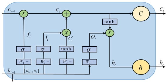
Figure 2. Multi-gating mechanism diagram.

(1)

Oblivion Gate

$${\mathrm{f}}_{\mathrm{t}}=\mathsf{\sigma }\left({\mathrm{W}}_{\mathrm{f}}\left[{\mathrm{h}}_{\mathrm{t}-1},{\mathrm{x}}_{\mathrm{t}}\right]+{\mathrm{b}}_{\mathrm{f}}\right)$$

(9)

where $h_{t-1}$ is the last moment hidden state and $x_t$ is the current input; $W_f$ and $b_f$ are the weight matrix and bias, respectively; and $\sigma$ is the Sigmoid activation function.

(2)

Input Gate and Candidate Memory

$${\mathrm{i}}_{\mathrm{t}}=\mathsf{\sigma }\left({\mathrm{W}}_{\mathrm{i}}\left[{\mathrm{h}}_{\mathrm{t}-1},{\mathrm{x}}_{\mathrm{t}}\right]+{\mathrm{b}}_{\mathrm{i}}\right)$$

(10)

$${\tilde{\mathrm{C}}}_{\mathrm{t}}=\mathrm{t}\mathrm{a}\mathrm{n}\mathrm{h}\left({\mathrm{W}}_{\mathrm{c}}\left[{\mathrm{h}}_{\mathrm{t}-1},{\mathrm{x}}_{\mathrm{t}}\right]+{\mathrm{b}}_{\mathrm{c}}\right)$$

(11)

where ${\tilde{C}}_t$ is the candidate memory state; $W_i,W_c$ and $b_i,b_c$ are the corresponding weights and biases; and $\mathrm{t}\mathrm{a}\mathrm{n}\mathrm{h}$ is the hyperbolic tangent function.

(3)

Memory unit update and output

$${\mathrm{C}}_{\mathrm{t}}={\mathrm{f}}_{\mathrm{t}}\cdot {\mathrm{C}}_{\mathrm{t}-1}+{\mathrm{i}}_{\mathrm{t}}\cdot {\tilde{\mathrm{C}}}_{\mathrm{t}}$$

(12)

$${\mathrm{o}}_{\mathrm{t}}=\mathsf{\sigma }\left({\mathrm{W}}_{\mathrm{o}}\left[{\mathrm{h}}_{\mathrm{t}-1},{\mathrm{x}}_{\mathrm{t}}\right]+{\mathrm{b}}_{\mathrm{o}}\right)$$

(13)

$${\mathrm{h}}_{\mathrm{t}}={\mathrm{o}}_{\mathrm{t}}\cdot \mathrm{t}\mathrm{a}\mathrm{n}\mathrm{h}\left({\mathrm{C}}_{\mathrm{t}}\right)$$

(14)

where $C_t$ is the current memory cell; $h_t$ is the current hidden state, which is used to predict or pass to the next moment; $W_o$ and $b_o$ are the weight and bias parameters.

LSTM can extract deep features with dynamic memory properties during gated modeling of time series, which are passed as inputs to iTransformer in the framework of this paper to further complete the modeling of global dependencies and feature fusion.

3.3. iTransformer

In multivariate time series prediction tasks, transformer, as one of the most important deep learning architectures in recent years, is widely used in load forecasting, energy scheduling, traffic flow modeling, etc., as it can model dependencies globally by means of the Self-Attention mechanism. All variables are spliced into a token input:

$${\mathrm{z}}_{\mathrm{t}}=\left[{\mathrm{x}}_{\mathrm{t}}^{\left(1\right)},{\mathrm{x}}_{\mathrm{t}}^{\left(2\right)},\dots ,{\mathrm{x}}_{\mathrm{t}}^{\left(\mathrm{N}\right)}\right]$$

(15)

$$\mathrm{Z}=\left[{\mathrm{z}}_1,{\mathrm{z}}_2,\dots ,{\mathrm{z}}_{\mathrm{T}}\right]$$

(16)

where $T$ is the number of time steps, $N$ is the number of variables, and $x_t^{\left(i\right)}$ denotes the observed value of the ith variable at time $t$.

This approach can work better when the sequence length is short, but in complex multivariate prediction tasks the following problems are encountered:

(1)

Variable interactions are implicitly realized. The attention weighting matrix is as the following:

$${\mathrm{A}}^{\mathrm{t}\mathrm{i}\mathrm{m}\mathrm{e}}=\mathrm{S}\mathrm{o}\mathrm{f}\mathrm{t}\mathrm{m}\mathrm{a}\mathrm{x}\left({\displaystyle \frac{\mathrm{Q}{\mathrm{K}}^{\top }}{\sqrt{{\mathrm{d}}_{\mathrm{k}}}}}\right),\mathrm{Q},\mathrm{K}\in {\mathbb{R}}^{\mathrm{T}\times {\mathrm{d}}_{\mathrm{k}}}$$

(17)

where $Q$ is the query matrix, $K$ is the key matrix, the dimensions of both are $T\times d_k, d_k$ is the dimension of the query and key vectors; $\sqrt{d_k}$ is the square root of the dimension of the key vector, used as a scaling factor. $\mathrm{S}\mathrm{o}\mathrm{f}\mathrm{t}\mathrm{m}\mathrm{a}\mathrm{x}(\cdot )$ denotes the Softmax function. $A^{\mathrm{time} }$ represents the correlation between different time steps, while the relationship between variables only exists implicitly within the same token, which is difficult to manifest explicitly, resulting in insufficient ability to model the coupling of multi-source input features.

(2)

Time–variable overlap: Time-step tokens contain multiple variables, which lead to the model facing both time and variable dimensions when learning dependencies, and the information is overlapped, making it difficult for the model to distinguish between time relevance and variable relevance’, thus affecting the generalization performance. The generalization performance is affected.

To cope with the above problem, iTransformer (inverted transformer) employs an inversion modeling paradigm. Variables rather than time steps are defined as tokens, and the complete history sequence of each variable is embedded as an independent representation. As a result, the domain of the self-attention mechanism is shifted from the time dimension to the variable dimension. This structural adjustment allows the model to explicitly portray cross-variate dependencies at the representational level and effectively mitigate the complexity of the long-series condition at the computational level.

(1)

Modeling

The overall structure of iTransformer follows the encoder framework of transformer, including the input embedding layer, the stacked transformer blocks, and the prediction projection layer, but it is significantly different from the traditional transformer in terms of token definition and the dimension of the role of the attention. Its core process can be represented as the following:

$$\begin{array}{c}{\mathrm{h}}_{\mathrm{i}}^{\left(0\right)}=\mathrm{E}\mathrm{m}\mathrm{b}\mathrm{e}\mathrm{d}\mathrm{d}\mathrm{i}\mathrm{n}\mathrm{g}\left({\mathrm{x}}^{\left(\mathrm{i}\right)}\right),\mathrm{i}=1,\dots ,\mathrm{N}\hfill \\ {\mathrm{H}}^{\left(0\right)}=\left[{\mathrm{h}}_1^{\left(0\right)},{\mathrm{h}}_2^{\left(0\right)},\dots ,{\mathrm{h}}_{\mathrm{N}}^{\left(0\right)}\right]\in {\mathbb{R}}^{\mathrm{N}\times \mathrm{D}}\hfill \\ {\mathrm{H}}^{(\mathrm{l}+1)}=\mathrm{T}\mathrm{r}\mathrm{m}\mathrm{B}\mathrm{l}\mathrm{o}\mathrm{c}\mathrm{k}\left({\mathrm{H}}^{\left(\mathrm{l}\right)}\right),\mathrm{l}=0,\dots ,\mathrm{L}-1\hfill \\ {\widehat{\mathrm{y}}}_{\mathrm{i}}=\mathrm{P}\mathrm{r}\mathrm{o}\mathrm{j}\mathrm{e}\mathrm{c}\mathrm{t}\mathrm{i}\mathrm{o}\mathrm{n}\left({\mathrm{h}}_{\mathrm{i}}^{\left(\mathrm{L}\right)}\right),\mathrm{i}=1,\dots ,\mathrm{N}\hfill \end{array}$$

(18)

where $h_i^{\left(0\right)}$ denotes the initial representation vector of the $i$th input and $x^{\left(i\right)}$ denotes the $i$th input sample; $H^{\left(0\right)}$ denotes the matrix consisting of all the initial representations, and $H^{\left(l\right)}$ denotes the hidden representation matrix of the $l$th layer; ${\widehat{y}}_i$ denotes the predicted output corresponding to the $i$th input, and $h_i^{\left(L\right)}$ denotes the $L$th layer at which this input becomes the representation vector. $\mathrm{Embedding}(\cdot )$ is used to embed the time series of each variable as a vector; $\mathrm{T}\mathrm{r}\mathrm{m}\mathrm{b}\mathrm{l}\mathrm{o}\mathrm{c}\mathrm{k}(\cdot )$ includes self-attention, feedforward networks, residual connectivity, and normalization; $\mathrm{Projection}(\cdot )$ is used for the output prediction layer. The difference with the traditional structure is that the number of input tokens is equal to the number of variables $N$, instead of time steps T. The idea is shown in Figure 3.

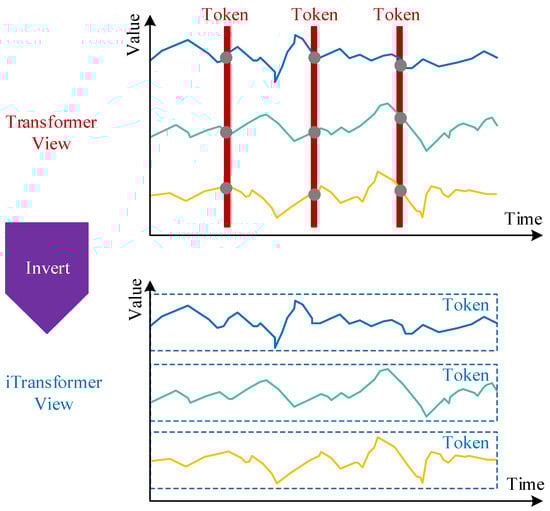
Figure 3. Overall structure of iTransformer. In the traditional Transformer view (top), tokens are constructed along the temporal axis, with each token corresponding to all variables at a specific time step; the grey dots represent local fluctuations or noise. In the iTransformer view (bottom), each variable is treated as an independent token, and this structure places greater emphasis on the dependencies among variables.

(2)

Input embedding and hierarchical characterization

Let the multivariate time series be

$$\mathrm{X}=\left\{{\mathrm{x}}^{\left(1\right)},{\mathrm{x}}^{\left(2\right)},\dots ,{\mathrm{x}}^{\left(\mathrm{N}\right)}\right\}$$

(19)

$${\mathrm{x}}^{\left(\mathrm{i}\right)}=\left[{\mathrm{x}}_1^{\left(\mathrm{i}\right)},{\mathrm{x}}_2^{\left(\mathrm{i}\right)},\dots ,{\mathrm{x}}_{\mathrm{T}}^{\left(\mathrm{i}\right)}\right].$$

(20)

The iTransformer projects each $x^{\left(i\right)}$ into a token:

$${\mathrm{h}}_{\mathrm{i}}^{\left(0\right)}=\mathrm{E}\mathrm{m}\mathrm{b}\mathrm{e}\mathrm{d}\mathrm{d}\mathrm{i}\mathrm{n}\mathrm{g}\left({\mathrm{x}}^{\left(\mathrm{i}\right)}\right)$$

(21)

where $h_i^{\left(0\right)}\in {\mathbb{R}}^D$ and D is the embedding dimension. This process compresses dynamic patterns (e.g., periodicity, trend) in the time dimension into token representations, allowing the subsequent attention mechanism to focus only on the interactions between variables.

This hierarchical representation idea has two advantages: on one hand, temporal dependence is modeled in the embedding stage, avoiding variable dependence being masked within temporal tokens; on the other hand, different variables are projected into the same representation space, reducing the impact of differences in measurement units and statistical distributions, and laying a unified feature base for subsequent attention operations.

(3)

Self-attention mechanism for variable dimensions

In the $l$th layer transformer block, the input is $H^{\left(l\right)}\in {\mathbb{R}}^{N\times D}$. It is obtained by linear mapping:

$$\mathrm{Q}={\mathrm{W}}_{\mathrm{Q}}{\mathrm{H}}^{\left(\mathrm{l}\right)},\mathrm{K}={\mathrm{W}}_{\mathrm{K}}{\mathrm{H}}^{\left(\mathrm{l}\right)},\mathrm{V}={\mathrm{W}}_{\mathrm{V}}{\mathrm{H}}^{\left(\mathrm{l}\right)}$$

(22)

where $W_Q,W_K,W_V\in {\mathbb{R}}^{D\times d_k}$, denote the projection parameter matrices of queries, keys, and values, respectively.

The attention weight matrix is as the following:

$${\mathrm{A}}^{\mathrm{v}\mathrm{a}\mathrm{r}}=\mathrm{S}\mathrm{o}\mathrm{f}\mathrm{t}\mathrm{m}\mathrm{a}\mathrm{x}\left({\displaystyle \frac{\mathrm{Q}{\mathrm{K}}^{\top }}{\sqrt{{\mathrm{d}}_{\mathrm{k}}}}}\right),{\mathrm{A}}^{\mathrm{v}\mathrm{a}\mathrm{r}}\in {\mathbb{R}}^{\mathrm{N}\times \mathrm{N}}.$$

(23)

The output is as the following:

$$\mathrm{O}={\mathrm{A}}^{\mathrm{v}\mathrm{a}\mathrm{r}}\mathrm{V}.$$

(24)

Unlike traditional transformers, $A_{ij}^{\mathrm{v}\mathrm{a}\mathrm{r}}$ explicitly represents the strength of dependence between the $i$th variable and the $j$th variable, thus enabling direct modeling of cross-variable interactions. In contrast, standard attention matrices can only portray correlations between moments, and variable interactions are implied within tokens, which lacks transparency.

(4)

Feedforward and residual structure

Attentional output was further mapped via a Feed-Forward Network (FFN):

$${\mathrm{H}}^{(\mathrm{l}+1)}=\mathrm{F}\mathrm{F}\mathrm{N}\left(\mathrm{O}\right)+{\mathrm{H}}^{\left(\mathrm{l}\right)}$$

(25)

where $\mathrm{F}\mathrm{F}\mathrm{N}(·)$ is a two-layer fully connected and nonlinear activation function. Residual connectivity with Layer Normalization (LN) ensures training stability when deep stacking and uniform distribution in variable dimensions to enhance comparability of cross-variate features.

In summary, the main difference in iTransformer is the redesign of the way tokens are defined: from a timestep-centric representation to a variable-centric representation. This structural adjustment theoretically provides a new modeling perspective for the portrayal of multivariate dependencies:

(1)

Time-variant hierarchical decoupling

iTransformer models temporal features in the embedding phase and variable features in the attention phase, which avoids conflation between the two and helps to improve the generalization of the model in non-smooth, multi-source input environments.

(2)

Multi-source feature fusion

Variables from different sources (e.g., weather, load, and renewable power) are unified into the attention mechanism at the token level, and the model can naturally capture cross-modal and cross-physical coupling relationships.

3.4. Hybrid Cosine Attention Mechanism

In the standard self-attention mechanism, the correlation between the query and the key is computed by scaling the dot product and normalized by the Softmax function to generate the attention weights. However, in multivariate time-series prediction tasks, the score function of this form not only relies on the directional relationship between the vectors but is also directly affected by the vector paradigms $‖q_i‖,‖k_j‖$.

This dependence may lead to systematic biases in the distribution of attention weights for different magnitude variables and exacerbate numerical stability problems under high-dimensional input conditions.

To alleviate the challenges, this paper proposes a hybrid cosine attention mechanism. The core idea of this mechanism is to normalize the query and key vectors to portray their relevance with cosine similarity. Therefore, temperature scaling and sparse gating are introduced before Softmax normalization to improve the numerical stability of the attention distribution and enhance the suppression of noise features. Its mathematical form is as the following:

$$\begin{array}{c}{\mathrm{A}}^{\mathrm{var} }=\mathrm{S}\mathrm{o}\mathrm{f}\mathrm{t}\mathrm{m}\mathrm{a}\mathrm{x}\left({\displaystyle \frac{\widehat{\mathrm{Q}}{\widehat{\mathrm{K}}}^{\top }}{\mathrm{\tau }}}+\mathrm{l}\mathrm{o}\mathrm{g}(\mathrm{G}+\mathsf{\delta })+\mathrm{M}\right),{\mathrm{A}}^{\mathrm{var} }\in {\mathbb{R}}^{\mathrm{N}\times \mathrm{N}} \\ \mathrm{Y}={\mathrm{A}}^{\mathrm{var} }\mathrm{V} \end{array}$$

(26)

where $\widehat{Q},\widehat{ K}$ are the normalized query and key matrices, respectively; $\tau >0$ is a temperature parameter to regulate the sharpness of the Softmax distribution; $G\in {\mathbb{R}}^N$ is the key-side non-negative gating, $\delta >0$ is a stability constant, and $\mathrm{l}\mathrm{o}\mathrm{g}(G+\delta )$ is used to suppress the invalidated or noisy features; $M$ is the masking matrix to prevent the future information leakage and padding position nullification; $V$ is the value matrix and the output is $Y$.

The hybrid cosine attention mechanism is more suitable for complex multivariate time series prediction tasks because it retains the characteristics of Softmax focusing and normalization, as well as numerical stability, controllability of distribution, and noise immunity.

4. Data Processing and Evaluation Indicators

4.1. Experimental Data

The experimental data used in this study were obtained from actual operating records of a regional power grid in northern China during a summer high-temperature period. The dataset covers 40 consecutive days in 2023, consisting of 3840 sampling points of total system active load, together with synchronously collected meteorological observations. In addition, to further examine the generalization capability of the proposed model across different regional load characteristics, load datasets from other regions were incorporated. These datasets contain continuous day-scale real-world measurements and serve as supplementary benchmarks for cross-regional validation. The load data were recorded by the dispatch center’s SCADA system at a 15-min interval and released after undergoing standard data-quality control procedures, including anomaly detection, timestamp alignment, and missing-value inspection. The meteorological data include the average air temperature and were collected by the local automatic weather station, with the same sampling frequency as the load to ensure temporal consistency and channel synchronization. Before model development, anomaly detection was applied to the raw load and meteorological time series using a combination of the interquartile range (IQR) method and three-times median absolute deviation (3 × MAD) to remove transient outliers caused by sensor drift or communication loss. Missing values were imputed using nearest-neighbor temporal interpolation.

4.2. Raw Data Decomposition and Normalization

The cleaned load series was decomposed using ICEEMDAN to obtain eight intrinsic mode functions (IMFs) and one residual component, as shown in Figure 4, which were then concatenated with the meteorological feature to form a multi-dimensional feature set. Samples were constructed using a sliding window of length $L$, where the corresponding IMF-meteorology matrix within each window served as the model input, and the load value at the next time step was used as the supervisory target. The dataset was partitioned chronologically into training (70%), validation (15%), and test (15%) subsets to preserve the temporal dependencies and prevent any leakage of future information. Subsequently, the load series and meteorological features were precisely aligned by timestamps to construct a unified multivariate input matrix.

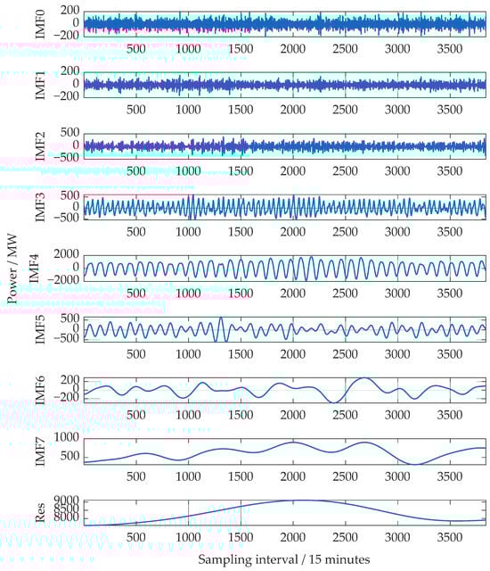
Figure 4. Decomposition process of raw load sequence with ICEEMDAN.

After completing the decomposition of the original load sequence, to eliminate the adverse effects of different scales and value ranges on the model training process, this paper carries out normalization pre-processing on the load and meteorological feature data. This operation can avoid the model convergence difficulties caused by the difference in numerical scales and enhance the comparability of different features in the modeling process. In this paper, the min-max normalization method is used to map each feature to the interval [0, 1], which is calculated as follows:

$${\mathrm{x}}^{\prime }={\displaystyle \frac{\mathrm{x}-{\mathrm{x}}_{\mathrm{m}\mathrm{i}\mathrm{n}}}{{\mathrm{x}}_{\mathrm{m}\mathrm{a}\mathrm{x}}-{\mathrm{x}}_{\mathrm{m}\mathrm{i}\mathrm{n}}}}$$

(27)

where $x$ denotes the original data, $x^{\prime }$ is the normalized data, $x_{min}$ and $x_{max}$ are the minimum and maximum values of the feature in the sample set, respectively. Through the normalization process, all input features are unified to the same scale, which ensures the stability of the training process.

4.3. Indicators for Model Evaluation

To measure the prediction performance of the model objectively and from multiple perspectives, this paper adopts four indicators, namely, the coefficient of determination (R²), the mean absolute error (MAE), the root mean square error (RMSE), and the mean absolute percentage error (MAPE). The above indicators can reflect the accuracy and stability of the prediction results in terms of goodness of fit, absolute deviation, mean square deviation and relative deviation, respectively. Their mathematical definitions are as follows:

$$\begin{array}{c}{\mathrm{R}}^2=1-{\displaystyle \frac{\sum _{\mathrm{i}=1}^{\mathrm{N}} {\left({\mathrm{y}}_{\mathrm{i}}-{\widehat{\mathrm{y}}}_{\mathrm{i}}\right)}^2}{\sum _{\mathrm{i}=1}^{\mathrm{N}} {\left({\mathrm{y}}_{\mathrm{i}}-\overline{\mathrm{y}}\right)}^2}}\\ \mathrm{M}\mathrm{A}\mathrm{E} ={\displaystyle \frac{1}{\mathrm{N}}}\sum _{\mathrm{i}=1}^{\mathrm{N}} \left|{\mathrm{y}}_{\mathrm{i}}-{\widehat{\mathrm{y}}}_{\mathrm{i}}\right|\\ \mathrm{R}\mathrm{M}\mathrm{S}\mathrm{E} =\sqrt{{\displaystyle \frac{1}{\mathrm{N}}}\sum _{\mathrm{i}=1}^{\mathrm{N}} {\left({\mathrm{y}}_{\mathrm{i}}-{\widehat{\mathrm{y}}}_{\mathrm{i}}\right)}^2}\\ \mathrm{M}\mathrm{A}\mathrm{P}\mathrm{E} ={\displaystyle \frac{100\%}{\mathrm{N}}}\sum _{\mathrm{i}=1}^{\mathrm{N}} \left|{\displaystyle \frac{{\mathrm{y}}_{\mathrm{i}}-{\widehat{\mathrm{y}}}_{\mathrm{i}}}{{\mathrm{y}}_{\mathrm{i}}}}\right|\end{array}$$

(28)

where $y_i$ is the true value, ${\widehat{y}}_i$ is the predicted value, $\overline{y}$ is the sample mean, and $N$ is the total number of samples.

5. Analysis of Experimental Results

5.1. Intermediate Representations and Visualization of Key Model Components

To provide a clearer understanding of how the proposed model extracts hierarchical features and captures cross-variable dependencies, this subsection visualizes the intermediate representations of its key modules, including the LSTM-based temporal feature mapping, the multi-head hybrid cosine-attention patterns, and the latent representations produced by the iTransformer encoder.

Figure 5 presents the hidden-state activations generated by the LSTM for the multi-scale IMF components, the residual term, and the meteorological variable. The horizontal axis denotes the time steps, the vertical axis corresponds to the input-variable dimension, and the color intensity indicates the activation magnitude. High-frequency IMFs exhibit rapidly fluctuating activation patterns, reflecting their pronounced influence on short-term load perturbations. In contrast, medium- and low-frequency IMFs form smoother, gradually evolving structures, corresponding to trend-related and cyclical behaviors. The residual term and temperature variable show distinct activation peaks at specific time positions, suggesting that the LSTM effectively captures the impact of exogenous drivers and non-decomposable components. Overall, the activations display a progressive temporal strengthening effect, demonstrating the LSTM’s ability to extract discriminative short-term dynamics from highly non-stationary load sequences and provide temporally structured features for the subsequent attention module.

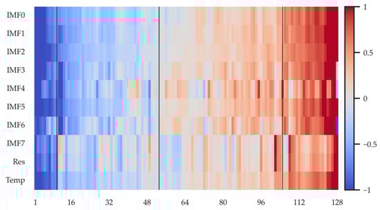
Figure 5. Hidden-state activations of the LSTM.

Figure 6 illustrates the hybrid cosine-attention weights of the four heads in the second attention layer, revealing the direction-normalized similarity structure among variables. The four heads exhibit clearly differentiated attention patterns: Heads 1 and 4 emphasize global coupling relationships, Head 2 focuses on interactions among medium-frequency components, and Head 3 concentrates on single-variable patterns. Such diversity indicates the inherent division of labor within the multi-head structure when modeling variable dependencies. Cosine normalization mitigates the norm bias caused by scale differences across IMFs, yielding more stable attention distributions that are not dominated by components with larger energy. The temperature-scaling factor further maintains a balanced trade-off between attention sharpness and dispersion, enabling more robust multi-scale dependency modeling.

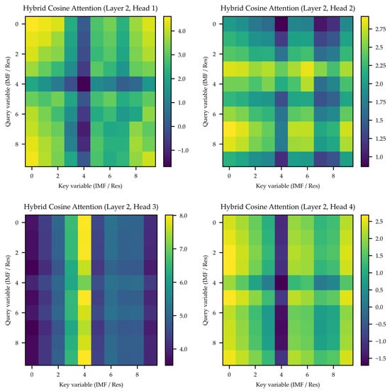
Figure 6. Multi-head hybrid cosine-attention patterns in the second attention layer.

Figure 7 shows the latent representations produced by the iTransformer encoder, where color indicates activation intensity in the high-dimensional embedding space. Compared with the localized temporal features extracted by the LSTM, these latent representations are smoother and more compact, suggesting that redundancy among IMF components is significantly reduced after attention-based aggregation. Local activation peaks appear at several time steps, indicating the encoder’s ability to identify and encode key variations in the load curve into a unified variable space. The overall representation is both balanced and concentrated, confirming that the iTransformer effectively establishes global variable-wise dependencies.

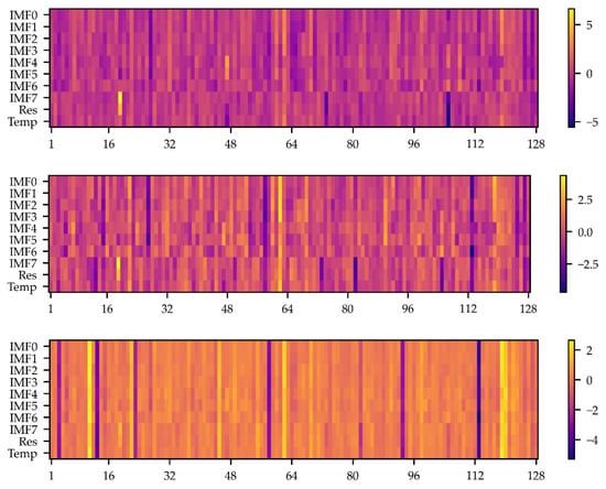
Figure 7. Latent representations generated by the iTransformer encoder (Block1-3).

5.2. Comparison Analysis with Traditional Models

To verify the effectiveness of the proposed method in the load forecasting task, four types of typical benchmark models are selected for comparison, namely RNN, LSTM, transformer, and iTransformer. All models are trained and tested with the same dataset and parameter settings, and the evaluation metrics are shown in Section 4.3. The experimental results of each model are shown in Table 1.

Table 1. Experimental results for each model.

	MAE	RMSE	MAPE	R2
RNN	206.48	253.20	2.34%	0.9394
LSTM	193.25	233.57	2.27%	0.9485
Transformer	187.63	225.32	2.21%	0.9521
iTransformer	190.54	229.57	2.23%	0.9502
Proposed Method	96.55	124.93	1.13%	0.9857

From the results in Table 1, the traditional neural network model can fit the load data better overall, but there are still obvious differences in the prediction task of complex non-stationary sequences. The performance of RNN is the most limited, with an R² of 0.9395, and the MAE and RMSE of 206.48 and 253.20, respectively, which indicates that the model is not capable of capturing the dependence of the long sequences and the nonlinear fluctuations. The LSTM model introduces a gating mechanism in its structure, which can alleviate the problem of gradient disappearance, and thus outperforms the RNN in all the indexes, in which the R² is improved to 0.9485, and the MAE and RMSE are reduced to 193.25 and 233.57, respectively, with improved prediction accuracy.

Further comparison of the transformer series of models based on the attention mechanism reveals that it exhibits stronger modeling capabilities in load forecasting. iTransformer has an R² of 0.9521, an MAE of 187.63, and an RMSE of 225.32, and performs better in portraying the long-time dependencies and capturing the global features compared to LSTM. iTransformer has improved in modeling multivariate interactions but is not as good as transformer in extracting serial dependencies in the time dimension, and thus performs slightly worse than transformer.

From Table 1, the proposed method is better than the comparison model in all the indicators. Its R² is 0.9857, MAE and RMSE are reduced to 96.55 and 124.93, which are about 48.6% and 44.6% lower than that of the second-best transformer, and MAPE is reduced to 1.13%, which is almost half of that of RNN. The data show that the proposed method has higher accuracy and stability in portraying both short-term fluctuations and long-term trends.

To demonstrate the accuracy of the proposed method in this paper more intuitively, the prediction results of the last 500 moments are selected for visualization and comparison, as shown in Figure 8. Overall, all models can portray the cyclical fluctuation characteristics of the load sequence, but there is an obvious difference in the fitting accuracy between the peak and valley intervals, as shown in Figure 8.

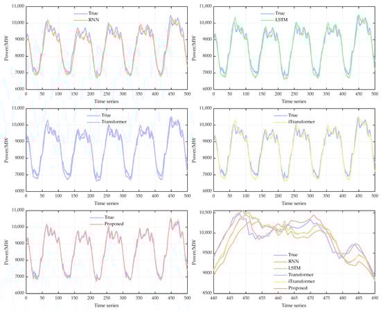
Figure 8. Comparison of the prediction results of different models.

Firstly, the prediction curves of RNN and LSTM are closer to the real curves in the overall trend but show a certain degree of lag and deviation in the zones of rapid load changes. Especially in the peak interval, the prediction results show underestimation phenomenon, which indicates that the cyclic class models are still deficient in capturing the long-time dependence and non-stationary fluctuations. Secondly, the prediction curves of transformer and iTransformer are overall more closely matched to the real values and can better reflect the peaks and valleys characteristics of the loads, which verifies the effectiveness of the attention mechanism in modeling long time span dependencies. However, iTransformer does not show any significant advantage over the standard transformer, and there is a slight bias in some of the valley intervals, which is related to its structural characteristic of emphasizing multivariate interaction modeling. In contrast, the prediction results of the proposed method in this paper are highly consistent with the real curve in all time periods, especially in the extreme value interval, which almost coincides with the real curve, and significantly reduces the prediction lag and bias. The results show that the proposed joint decomposition-local-global-stability modeling framework can effectively reduce the non-stationarity of the original load series and improve the characterization of multi-scale features, thus achieving better prediction performance at both the overall trend and local detail levels. The proposed decomposition-local-global-stability joint modeling framework can effectively reduce the non-stationarity of the original load series and improve the characterization of multi-scale features, thus obtaining better prediction performance in both the overall trend and local details.

Each model can converge faster during the training process (Figure 9), but the method proposed in this paper maintains the lowest loss level and the smallest fluctuation in the whole process, which indicates that it has a more significant advantage in optimization stability and generalization performance.

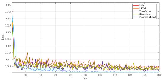
Figure 9. Comparison of training loss curves for different models.

5.3. Ablation Experiments

To further explore the contribution of each functional module in the proposed method to the overall performance, this section designs ablation experiments to gradually remove or replace key components of the model and construct different variants for comparison. The specific experimental setup includes the following:

iTransformer: Only the base iTransformer structure is used.

LSTM–iTrans–cosA: Adds an LSTM feature extraction layer before the iTransformer and introduces hybrid cosine attention.

ICEEMDAN–iTrans–cosA: Adopts ICEEMDAN decomposition as preprocessing but does not include the LSTM layer.

ICEEMDAN–LSTM–iTrans: Includes ICEEMDAN and LSTM but does not use hybrid cosine attention.

Proposed Method: Complete framework, i.e., ICEEMDAN + LSTM + iTransformer + hybrid cosine attention.

The experimental results are shown in Table 2.

Table 2. Experimental results for different models.

	MAE	RMSE	MAPE	R2
iTransformer	190.53	229.57	2.34%	0.9503
LSTMiTrans–cosAv	160.74	194.07	1.92%	0.9656
ICEEMDAN–iTrans–cosA	158.65	191.98	1.98%	0.9663
ICEEMDAN–LSTM–iTrans	119.37	150.34	1.40%	0.9793
Proposed Method	96.55	124.93	1.13%	0.9857

From the results, it can be observed that the standalone iTransformer exhibits certain limitations in forecasting accuracy, achieving an R² of only 0.9503, while its MAE and RMSE remain relatively high at 190.53 and 229.57, respectively. This indicates that when dealing with non-stationary load series, relying solely on global dependency modeling is insufficient to adequately capture local dynamic patterns. With the introduction of LSTM and the hybrid cosine attention mechanism, the model performance improves significantly: R² increases to 0.9656, while MAE and RMSE are reduced by 15.6% and 15.5%, respectively. This demonstrates the effectiveness of local temporal dependency extraction and stabilized attention distribution in controlling prediction errors. After incorporating ICEEMDAN decomposition, the error metrics further decrease, suggesting that weakening the non-stationarity of the series enhances the specificity and effectiveness of subsequent feature learning. When ICEEMDAN and LSTM are retained but the hybrid cosine attention mechanism is removed, the model still achieves a high level of fitting performance, with R² rising to 0.9793, indicating that the combination of decomposition and local modeling provides a fundamental contribution to overall performance improvement. Finally, the proposed model achieves the best results across all four-evaluation metrics, with an MAE of 96.55, an RMSE of 124.93, and an R² of 0.9857, validating its synergistic advantages in multi-scale feature representation and cross-level modeling.

When ICEEMDAN and LSTM are retained without introducing the hybrid cosine attention mechanism, the model still exhibits a high degree of goodness-of-fit, showing that the combination of decomposition and local modeling plays a fundamental role in the overall performance improvement. Ultimately, the proposed model achieves optimal results in all four metrics, which verifies the synergistic advantages of the proposed method in multi-scale feature characterization and cross-level modeling.

Figure 10 illustrates the comparison of different ablation models with the real load profile. The iTransformer alone can reproduce the general trend but shows significant deviations in the peak and trough intervals, indicating that it does not sufficiently characterize the local dynamics. After the introduction of LSTM and hybrid cosine attention mechanism, the response ability of the model is enhanced in the fast-varying region, and the temporal consistency of the prediction curves is improved. After combining the ICEEMDAN decomposition, the error is further narrowed in the extreme range, indicating that the decomposition plays a role in alleviating the non-stationarity. The overall fit is further improved when the joint structure of ICEEMDAN and LSTM is used. The predicted curves of the proposed model are highly consistent with the true curves and show excellent fits in both the overall shape and local details, as shown in Figure 10. The results are consistent with the quantitative indexes in Table 2, verifying the effectiveness and necessity of multi-module collaborative modeling.

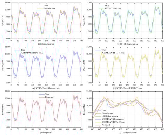
Figure 10. Comparison of predicted results from ablation experiments.

As can be seen from Figure 11, all models converge faster, but the complete ICEEMDAN–LSTM–iTransformer-hybrid cosine attention framework maintains the lowest loss level almost throughout, reflecting stronger training stability and generalization ability.

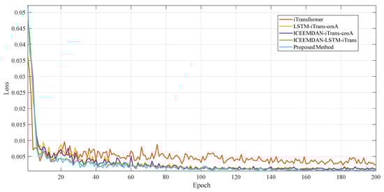
Figure 11. Comparison of training loss curves for ablation experiments.

5.4. Statistical Significance Testing and Sensitivity Analysis

As shown in Table 3, the proposed method achieves extremely small p-values in both paired t-tests and Wilcoxon signed-rank tests when compared with all seven baseline models. Specifically, the t-test p-values range from 5.18793 × 10⁻⁵³ to 7.91437 × 10⁻¹², while the Wilcoxon p-values range from 4.25252 × 10⁻⁴⁵ to 2.20031 × 10⁻¹⁰. All values are far below the significance threshold of 0.05, demonstrating that the performance improvements of the proposed framework are statistically significant at the 95% confidence level. These results confirm that the superiority of the proposed model is systematic rather than arising from random fluctuations in the dataset.

Table 3. Results of statistical significance testing.

Model Comparison	t-Test p-Value	Wilcoxon p-Value
RNN	3.92028 × 10−44	6.80514 × 10−39
LSTM	1.37148 × 10−50	1.28162 × 10−43
Transformer	5.18793 × 10−53	4.25252 × 10−45
iTransformer	4.07633 × 10−52	2.63853 × 10−44
LSTM–iTrans–cosA	1.38485 × 10−43	2.59469 × 10−38
ICEEMDAN–iTrans–cosA	1.50752 × 10−43	3.5088 × 10−38
ICEEMDAN–LSTM–iTrans	7.91437 × 10−12	2.20031 × 10−10

The sensitivity analysis is performed around the final configuration, where the historical input window length is set to look_back = 96, the batch size is 128, the learning rate is 5 × 10⁻³, the embedding/representation dimension is d_model = 128, the number of attention heads is n_heads = 4, the number of encoder layers is n_layers = 3, the feed-forward network width is dim_ffn = 4 × d_model, the dropout rate is 0.1, and the τ = 0.1. We perturb one hyperparameter at a time and keep the others fixed to observe how the prediction accuracy reacts to controlled structural changes. Table 4 reports the evaluation metrics under different hyperparameter settings.

Table 4. Results of the sensitivity analysis.

	MAE	RMSE	MAPE	R2
Look_back = 48	177.75	221.42	2.04%	0.9542
Look_back = 144	136.71	175.10	1.58%	0.9719
d_model = 144	164.71	209.47	1.91%	0.9615
d_model = 256	147.67	186.42	1.72%	0.9695
τ = 0.05	235.41	277.04	2.72%	0.9326
τ = 0.2	180.95	228.43	2.08%	0.9542
Optimal parameters	96.55	124.93	1.13%	0.9857

Although the evaluation metrics deteriorate when deviating from the optimal configuration, the degradation shows no abnormal jumps and remains within a small and stable range. This indicates that the model exhibits neither instability nor sensitivity explosion, and its overall performance remains stable under hyperparameter perturbations, demonstrating strong robustness.

5.5. Evaluation of Model Performance on External Datasets

To further evaluate the generalization capability of the proposed model, we conduct additional experiments on two external datasets. As summarized in Table 5, the model maintains consistently high prediction accuracy across both datasets. Specifically, it achieves MAE values of 195.94 and 146.38, RMSE values of 262.40 and 173.12, MAPE values of 2.82% and 1.73%, and R² scores of 0.9648 and 0.9744 on Data 1 and Data 2, respectively. These results demonstrate that the model delivers stable and robust performance on datasets with different temporal patterns, confirming its strong applicability beyond the primary training set. Figure 12 illustrates the model’s prediction performance on two additional datasets (Data 1 and Data 2). In both cases, the predicted curves closely follow the ground-truth values, demonstrating the model’s strong generalization capability across datasets.

Table 5. Validation results on additional datasets.

	MAE	RMSE	MAPE	R2
Data 1	195.94	262.40	2.82%	0.9648
Data 2	146.38	173.12	1.73%	0.9744

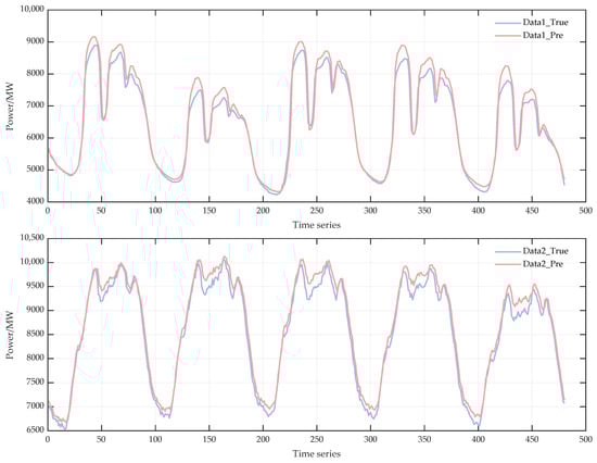
Figure 12. Performance on other datasets.

6. Conclusions

In this paper, a hierarchical forecasting framework integrating ICEEMDAN–LSTM–iTransformer with hybrid attention mechanism is proposed to address the problems of strong non-stationarity, complex multi-scale features, and insufficient modeling of cross-variate dependence that are commonly found in short-term electricity load forecasting. The method uses ICEEMDAN decomposition to reduce the non-stationarity of the sequence and extract the multi-timescale information at the input stage, combines with LSTM module to enhance the characterization of local nonlinear dynamics and short-term dependence, and then realizes the explicit modeling of cross-variable interactions and global dependence through the iTransformer architecture, and at the same time, introduces the cosine normalization improvement in the attention mechanism to enhance the numerical stability and cross-scale information aggregation.

In the arithmetic example based on real load data, the comparison experiment proves the effectiveness of the constructed framework, while the ablation experiment further reveals the independent contributions of the modules in different dimensions and their synergistic effects. The experimental results verify the advantages of the proposed method in terms of forecasting accuracy and stability, demonstrating that the obtained short-term load predictions can directly support practical power system operations. More accurate short-term load forecasts help improve the quality of rolling schedules in real-time dispatch, reduce uncertainty in reserve allocation, and provide more reliable prior load information for renewable energy accommodation, thereby enhancing operational flexibility and security margins under highly volatile conditions.

Future work could be carried out in the following areas: First, graph neural networks can be used to better characterize the spatial coupling properties of the power system and to realize spatial and temporal integrated prediction. Second, external perturbations such as extreme weather and demand-side response are considered to enhance the robustness of the model in abnormal situations. Third, the lightweight and online update mechanism of the model is explored to meet the real-time and deployable requirements of the actual grid operation. Building on this foundation, a more comprehensive research route may be further developed, including multi-regional forecasting, probabilistic prediction, and risk-aware scheduling, as well as integrated prediction–control frameworks, to facilitate the deployment of data-driven forecasting models in future renewable-dominated power systems.

References

- Wang, C.; Zhao, H.; Liu, Y.; Fan, G. Minute-level ultra-short-term power load forecasting based on time series data features. Appl. Energy 2024, 372, 123801. [Google Scholar] [CrossRef]
- Dai, Y.; Yu, W. Short-term power load forecasting based on Seq2Seq model integrating Bayesian optimization, temporal convolutional network and attention. Appl. Soft Comput. 2024, 166, 112248. [Google Scholar] [CrossRef]
- Chen, X.; Liu, Y.; Zhong, Z.; Fan, N.; Zhao, Z.; Wu, L. A carryover storage valuation framework for medium-term cascaded hydropower planning: A Portland General Electric system study. IEEE Trans. Sustain. Energy 2025, 16, 1903–1918. [Google Scholar] [CrossRef]
- Jia, X.; Xia, Y.; Yan, Z.; Gao, H.; Qiu, D.; Guerrero, J.M.; Li, Z. Coordinated operation of multi-energy microgrids considering green hydrogen and congestion management via a safe policy learning approach. Appl. Energy 2025, 401 Pt A, 126611. [Google Scholar] [CrossRef]
- Chan, K.Y.; Yiu, K.F.C.; Kim, D.; Abu-Siada, A. Fuzzy Clustering-Based Deep Learning for Short-Term Load Forecasting in Power Grid Systems Using Time-Varying and Time-Invariant Features. Sensors 2024, 24, 1391. [Google Scholar] [CrossRef] [PubMed]
- Kong, X.; Wang, Z.; Xiao, F.; Bai, L. Power load forecasting method based on demand response deviation correction. Int. J. Electr. Power Energy Syst. 2023, 148, 109013. [Google Scholar] [CrossRef]
- Zheng, Z.; Chen, H.; Luo, X. A Kalman filter-based bottom-up approach for household short-term load forecast. Appl. Energy 2019, 250, 882–894. [Google Scholar] [CrossRef]
- Cao, Z.; Wang, J.; Xia, Y. Combined electricity load-forecasting system based on weighted fuzzy time series and deep neural networks. Eng. Appl. Artif. Intell. 2024, 132, 108375. [Google Scholar] [CrossRef]
- Wang, J.; Zhang, L.; Li, Z. Interval forecasting system for electricity load based on data pre-processing strategy and multi-objective optimization algorithm. Appl. Energy 2022, 305, 117911. [Google Scholar] [CrossRef]
- Pappas, S.; Ekonomou, L.; Karampelas, P.; Karamousantas, D.; Katsikas, S.; Chatzarakis, G.; Skafidas, P. Electricity demand load forecasting of the Hellenic power system using an ARMA model. Electr. Power Syst. Res. 2010, 80, 256–264. [Google Scholar] [CrossRef]
- Dubey, A.K.; Kumar, A.; García-Díaz, V.; Sharma, A.K.; Kanhaiya, K. Study and analysis of SARIMA and LSTM in forecasting time series data. Sustain. Energy Technol. Assess. 2021, 47, 101474. [Google Scholar] [CrossRef]
- Li, Y.; Han, D.; Yan, Z. Long-term system load forecasting based on data-driven linear clustering method. J. Mod. Power Syst. Clean Energy 2018, 6, 306–316. [Google Scholar] [CrossRef]
- Chodakowska, E.; Nazarko, J.; Nazarko, Ł. ARIMA Models in Electrical Load Forecasting and Their Robustness to Noise. Energies 2021, 14, 7952. [Google Scholar] [CrossRef]
- Dong, X.; Deng, S.; Wang, D. A short-term power load forecasting method based on k-means and SVM. J. Ambient. Intell. Humaniz. Comput. 2022, 13, 5253–5267. [Google Scholar] [CrossRef]
- Jiang, Z.; Peng, J.; Yin, R.; Hu, M.; Cao, J.; Zou, B. Stochastic modelling of flexible load characteristics of split-type air conditioners using grey-box modelling and random forest method. Energy Build. 2022, 273, 112370. [Google Scholar] [CrossRef]
- Liu, F.; Liang, C. Short-term power load forecasting based on AC-BiLSTM model. Energy Rep. 2024, 11, 1570–1579. [Google Scholar] [CrossRef]
- Han, J.; Zeng, P. Short-term power load forecasting based on hybrid feature extraction and parallel BiLSTM network. Comput. Electr. Eng. 2024, 119 Pt B, 109631. [Google Scholar] [CrossRef]
- Abumohsen, M.; Owda, A.Y.; Owda, M. Electrical Load Forecasting Using LSTM, GRU, and RNN Algorithms. Energies 2023, 16, 2283. [Google Scholar] [CrossRef]
- Zelios, V.; Mastorocostas, P.; Kandilogiannakis, G.; Kesidis, A.; Tselenti, P.; Voulodimos, A. Short-Term Electric Load Forecasting Using Deep Learning: A Case Study in Greece with RNN, LSTM, and GRU Networks. Electronics 2025, 14, 2820. [Google Scholar] [CrossRef]
- Wen, L.; Zhou, K.; Li, J.; Wang, S. Modified deep learning and reinforcement learning for an incentive-based demand response model. Energy 2020, 205, 118019. [Google Scholar] [CrossRef]
- Wan, A.; Chang, Q.; Al-Bukhaiti, K.; He, J. Short-term power load forecasting for combined heat and power using CNN-LSTM enhanced by attention mechanism. Energy 2023, 282, 128274. [Google Scholar] [CrossRef]
- Fan, C.; Nie, S.; Xiao, L.; Yi, L.; Wu, Y.; Li, G. A multi-stage ensemble model for power load forecasting based on decomposition, error factors, and multi-objective optimization algorithm. Int. J. Electr. Power Energy Syst. 2024, 155 Pt B, 109620. [Google Scholar] [CrossRef]
- Lim, B.; Arık, S.Ö.; Loeff, N.; Pfister, T. Temporal Fusion Transformers for interpretable multi-horizon time series forecasting. Int. J. Forecast. 2021, 37, 1748–1764. [Google Scholar] [CrossRef]
- Vaswani, A.; Shazeer, N.; Parmar, N.; Uszkoreit, J.; Jones, L.; Gomez, A.N.; Kaiser, Ł.; Polosukhin, I. Attention is all you need. arXiv 2017. [Google Scholar] [CrossRef]
- Zhou, H.; Zhang, S.; Peng, J.; Zhang, S.; Li, J.; Xiong, H.; Zhang, W. Informer: Beyond efficient transformer for long sequence time-series forecasting. Proc. AAAI Conf. Artif. Intell. 2021, 35, 11106–11115. [Google Scholar] [CrossRef]
- Wu, H.; Xu, J.; Wang, J.; Long, M. Autoformer: Decomposition Transformers with auto-correlation for long-term series forecasting. arXiv 2021, arXiv:2106.13008. [Google Scholar] [CrossRef]
- Zhou, T.; Ma, Z.; Wen, Q.; Wang, X.; Sun, L.; Jin, R. FEDformer: Frequency enhanced decomposed transformer for long-term series forecasting. arXiv 2022, arXiv:2201.12740. Available online: https://arxiv.org/abs/2201.12740 (accessed on 28 November 2025). [CrossRef]
- Liu, J.; Yang, F.; Yan, K.; Jiang, L. Household energy consumption forecasting based on adaptive signal decomposition enhanced iTransformer network. Energy Build. 2024, 324, 114894. [Google Scholar] [CrossRef]
- Liu, Y.; Hu, T.; Zhang, H.; Wu, H.; Wang, S.; Ma, L.; Long, M. iTransformer: Inverted transformers are effective for time series forecasting. arXiv 2023, arXiv:2310.06625. [Google Scholar] [CrossRef]
- Pei, J.; Liu, N.; Shi, J.; Ding, Y. Tackling the duck curve in renewable power system: A multi-task learning model with iTransformer for net-load forecasting. Energy Convers. Manag. 2025, 326, 119442. [Google Scholar] [CrossRef]
- Qin, Z.; Sun, W.; Deng, H.; Li, D.; Wei, Y.; Lv, B.; Yan, J.; Kong, L.; Zhong, Y. CosFormer: Rethinking softmax in attention. In Proceedings of the International Conference on Learning Representations (ICLR 2022), Online, 25–29 April 2022. [Google Scholar]
- Xiong, Z.; Yao, J.; Huang, Y.; Yu, Z.; Liu, Y. A wind speed forecasting method based on EMD-MGM with switching QR loss function and novel subsequence superposition. Appl. Energy 2024, 353 Pt B, 122248. [Google Scholar] [CrossRef]
- Li, J.; Deng, D.; Zhao, J.; Cai, D.; Hu, W.; Zhang, M.; Huang, Q. A novel hybrid short-term load forecasting method of smart grid using MLR and LSTM neural network. IEEE Trans. Ind. Inform. 2021, 17, 2443–2452. [Google Scholar] [CrossRef]
- Ren, Y.; Suganthan, P.N.; Srikanth, N. A comparative study of empirical mode decomposition-based short-term wind speed forecasting methods. IEEE Trans. Sustain. Energy 2015, 6, 236–244. [Google Scholar] [CrossRef]
- Ma, K.; Nie, X.; Yang, J.; Zha, L.; Li, G.; Li, H. A power load forecasting method in port based on VMD-ICSS-hybrid neural network. Appl. Energy 2025, 377 Pt B, 124246. [Google Scholar] [CrossRef]
- Qin, C.; Qin, D.; Jiang, Q.; Zhu, B. Forecasting carbon price with attention mechanism and bidirectional long short-term memory network. Energy 2024, 299, 131410. [Google Scholar] [CrossRef]
Disclaimer/Publisher’s Note: The statements, opinions and data contained in all publications are solely those of the individual author(s) and contributor(s) and not of MDPI and/or the editor(s). MDPI and/or the editor(s) disclaim responsibility for any injury to people or property resulting from any ideas, methods, instructions or products referred to in the content. |
© 2025 by the authors. Licensee MDPI, Basel, Switzerland. This article is an open access article distributed under the terms and conditions of the Creative Commons Attribution (CC BY) license (https://creativecommons.org/licenses/by/4.0/).