Abstract
Accurate sea surface temperature (SST) forecasting in coastal upwelling systems requires predictive models capable of representing complex oceanic geometries. This work revisits grid-to-mesh coupling strategies in Graph Neural Networks (GNNs) and analyzes how mesh topology and connectivity influence prediction accuracy and artifact formation. This standard coupling process is a significant source of discretization errors and spurious numerical artifacts that compromise the final forecast’s accuracy. Using daily Copernicus SST and 10 m wind reanalysis data from 2000 to 2020 over the Canary Islands and the Northwest African region, we evaluate four mesh configurations under varying grid-to-mesh connection densities. We analyze two structured meshes and propose two new unstructured meshes for which their nodes are distributed according to the bathymetry of the ocean region. The results show that forecast errors exhibit geometric patterns equivalent to order-k Voronoi tessellations generated by the k-nearest neighbor association rule. Bathymetry-aware meshes with and grid-to-mesh connections significantly reduce polygonal artifacts and improve long-term coherence, achieving up to 30% lower relative to structured baselines. These findings reveal that the underlying geometry, rather than node count alone, governs error propagation in autoregressive GNNs. The proposed analysis framework provides a clear understanding of the implications of grid-to-mesh connections and establishes a foundation for artifact-aware, geometry-adaptive learning in operational oceanography.
1. Introduction
The monitoring and forecasting of oceanographic variables have gained increasing importance over the last decade across various disciplines, including oceanography, climatology, sustainable marine resource management, maritime navigation, and natural disaster mitigation. Variables such as sea surface temperature (SST), salinity, currents, and sea level are central to understanding the dynamic state of the ocean and its interactions with terrestrial and marine ecosystems [1,2,3].
Growing concerns about climate change and the intensification of extreme events—such as hurricanes, marine heatwaves, and rising sea levels—have created strong demand for fast, accurate, and computationally efficient predictive models to support decision-making in fisheries, maritime transport, marine conservation, and environmental policy.
Traditional physics-aware models provide a robust framework for simulating ocean dynamics, although limited by factors such as high computational costs, sensitivity to initial conditions, and the difficulty of representing complex marine environments on regular grids [4,5]. Deep learning methods have emerged as scalable alternatives for modeling oceanographic processes directly from observational data [6,7,8]. Among these, Graph Neural Networks (GNNs) are particularly well suited for geophysical applications, as they explicitly capture spatial relationships between observations through graph structures, offering flexibility for modeling localized and irregular phenomena [9,10].
Nevertheless, the performance of GNNs is strongly influenced by the interaction between the observational grid and the model’s latent mesh [11]. Observational data, such as SST, are typically defined on structured spatial grids, and the mesh adopts a more flexible topological structure. The way these two entities are coupled defines how efficiently information flows during message passing and ultimately determines predictive accuracy. Empirical evidence [12,13] shows that inadequate grid-to-mesh coupling can generate systematic prediction artifacts, including polygonal patterns and discontinuities across spatial tiles, which not only increase errors but also undermine the physical consistency and reliability of forecasts over longer horizons.
This is particularly significant in strategically important regions such as the Canary Islands and the northwest African coast, where the upwelling process drives high biological productivity and sustains valuable fisheries. Accurate and timely SST forecasts in these regions are vital for sustainable resource management and for anticipating ecosystem responses to climate variability [14,15]. The recurrent appearance of localized artifacts in SST prediction highlights a structural weakness in current graph architectures, as errors tend to accumulate at tile boundaries and propagate through the prediction horizon.
To address this problem, we propose a systematic experimental framework that explores how mesh design and connectivity patterns influence error dynamics in SST forecasting. Conceptually, the mesh embeds the forecasting process, while the grid defines the physical observational lattice. By varying the number of connections per node, redistributing mesh nodes according to spatial complexity, and analyzing the resulting error maps, we aim to uncover reproducible design principles that reduce artifacts and improve forecast coherence. Our approach leverages high-resolution satellite products from Copernicus Marine and Climate services [16], supported by auxiliary information such as bathymetry and land–sea separation to ensure physically consistent data representation.
The aim of this work is thus twofold: first, to quantify how grid-to-mesh connectivity influences the geometry and severity of prediction artifacts; and second, to evaluate how strategic mesh reconfigurations can reduce errors and enhance the spatial coherence of forecasts. Preliminary findings [11] indicate that connectivity plays a crucial role, with approximately four connections per node mitigating artifact formation under the evaluated conditions, while naively increasing node count alone does not guarantee improvement. Instead, performance gains arise from node distributions in regions most susceptible to error. These insights open the path toward more robust grid-to-mesh association mechanisms.
We explore four different mesh configurations. Starting from a structured and quadrangular structure [17], we propose a simplified version removing crossing edges. Then, we derive two new unstructured mesh configurations based on a probability distribution of the bathymetry: The first approach relies on a random distribution inversely proportional to the depth of the sea, whereas the second redistributes nodes more regularly to avoid a high concentration near the coast.
Our results show that the optimal number of grid-to-mesh connections depends on the type of mesh employed, and densifying the node distribution according to the seabed’s topology reduces artifacts and increases the accuracy of forecasts. The experiments demonstrate the better performance of bathymetry-based meshes with three and four connections, improving by 30% with respect to the structured mesh baselines.
Section 2 relates our work to the current state of the art, particularly in relation to forecasting with GNNs. In Section 3, we introduce the dataset and the geographical area of this study, as well as the different strategies employed for mesh generation. The results in Section 4 provide a detailed analysis of the influence of connections between the grid and the mesh in the generation of artifacts, as well as the importance of the number of nodes for improving accuracy. Finally, Section 5 and Section 6 report the discussion of results and present the main findings of this work.
2. Related Work
Predicting oceanographic variables represents one of the most complex challenges in contemporary marine sciences, requiring the integration of multiple disciplines ranging from fluid physics and atmospheric dynamics to advanced computational techniques and artificial intelligence methods. The ocean, as a dynamic system, exhibits behaviors that span time scales from seconds to decades and spatial scales from meters to entire ocean basins, thus demanding diverse and complementary methodological approaches for its understanding and forecasting [18].
Traditionally, predictive oceanography has been grounded in physical ocean modeling, employing fluid mechanics equations to describe ocean dynamics through general circulation models, which have proven effective over decades. However, the exponential development of artificial intelligence techniques and the massive availability of oceanographic data have fostered the emergence of deep-learning-based ocean modeling as a complementary—and in some cases, alternative—approach to traditional methods [19].
Deep-learning-based methods promise to overcome some inherent limitations of physical models, such as the parameterization of subscale processes and high computational costs, using algorithms that can learn complex representations directly from data. The ability of these techniques to learn nonlinear representations from large volumes of data has driven their application in tasks such as SST prediction, reconstruction of incomplete fields, identification of dynamic structures, and detection of extreme events, among others [20].
Convolutional Neural Networks (CNNs) are particularly suitable for working with oceanographic data. Their convolutional layers can automatically extract relevant spatiotemporal patterns by leveraging the strong spatial and temporal correlations in marine data. Temporal Convolutional Networks [21] have been shown to capture multi-scale temporal dependencies in SST time series, and the combination of SST with auxiliary variables [22,23], such as sea surface salinity, sea height, and ocean heat, helps improve reconstruction and extend forecast horizons. To address spatial heterogeneity, the Multi-Scale Bayesian CNN [24] models uncertainty across scales, and 3D architectures like the 3D U-Net CNN [25] and Spatiotemporal Siamese CNN [26] capture complex spatiotemporal patterns, including regional variations and marine heatwaves. More advanced models [27,28] incorporate four-dimensional convolutions to represent vertical and horizontal ocean structures, enhancing the spatial resolution of satellite SST maps.
Recurrent Neural Networks (RNNs) have been widely applied in oceanographic modeling due to their ability to capture complex temporal dependencies associated with seasonal and interannual variability. LSTM [29] and GRU [30] models are commonly used for the univariate and multivariate forecasting of oceanic variables. Hybrid approaches combining RNNs with Convolutional Neural Networks (CNNs) exploit CNNs for spatial feature extraction and RNNs for temporal modeling. In particular, ConvLSTM networks [31] have shown strong performance in spatiotemporal forecasting tasks, such as in SST and chlorophyll prediction [32,33]. Further extensions [34,35,36], enhance temporal learning through graph structures, semantic decomposition, and multi-source data integration. Attention-based architectures [37] and hierarchical models [38] improve feature selection and long-term forecasting stability. Additionally, the combination of CNN-GRU with multilayer perceptrons [39] for multiscale learning and spatial correlation modeling demonstrates the growing sophistication of RNN-based frameworks in ocean prediction tasks.
GNNs are particularly well-suited for oceanographic modeling because they naturally represent irregular spatial relationships among geographically dispersed locations [12]. In such models, nodes typically correspond to specific geographic positions, while edges encode physical or functional connections, enabling both node and edge features to capture complex spatiotemporal dependencies. Recent GNN-based approaches for SST prediction have leveraged these capabilities through diverse architectural designs. For instance, GNN-OAM [40] integrates multiple adjacency matrices and attention mechanisms to model three-dimensional spatiotemporal interactions; GMNN [10] combines a graph encoder with memory units to capture long-term temporal dependencies; DYGOV [41] introduces a dynamic graph that evolves in response to oceanic and meteorological conditions; HiGRN [42] employs hierarchical node clustering with multi-level attention to integrate local and global spatial patterns, achieving improved global SST prediction performance.
GNNs are particularly effective for modeling complex geographic regions such as coastal zones, archipelagos, and areas influenced by dynamic ocean currents [12,13,17]. The design of the mesh structure plays a pivotal role in balancing model accuracy and computational efficiency. Global models such as GraphCast [43] employ multiresolution icosahedral meshes to represent the entire planet, albeit at the cost of a high node count. In contrast, local models like HI-LAM [44] use rectangular meshes to focus on specific regions, while SeaCast [17] adapts mesh contours to irregular coastlines, such as those of the Mediterranean, while maintaining a regular grid structure. However, regular meshes may introduce visual artifacts at lower resolutions [12,13], and simply increasing the number of nodes does not necessarily improve predictive precision and can even degrade performance due to computational inefficiencies.
Rather than assuming that denser or bathymetry-aligned meshes inherently improve accuracy [11], our findings indicate that the dominant factor is the association geometry between grid and mesh. Even topology-aware graphs impose order-k Voronoi partitions that act as semi-isolated predictors, leading to structured temporal drift along tile boundaries. Physical gradients like bathymetry are useful only when employed to reshape connectivity or redistribute nodes where per-tile slopes are steep, as they are not used as standalone prescriptions for mesh design.
3. Materials and Methods
In this section, we introduce the dataset and the area of study used in this work, related to the Canary Islands and the Northwestern African coast. Then, we explain the GNN architecture and the different mesh configurations tested in this work. Finally, we comment on the experiments and metrics used in the results.
3.1. Dataset
The experimental dataset is a spatiotemporal series of SST and wind fields over the Canary Islands region, derived from the Copernicus Marine Service Program and the European Centre for Medium-Range Weather Forecasts, respectively. Specifically, we use the SST reanalysis product [45], which provides daily observations at a spatial resolution of 0.05. SST is a key physical variable for detecting upwelling processes and understanding coastal dynamics.
To complement SST, we incorporate wind data at 10 m above the surface, using the zonal (east–west) and meridional (north–south) components [46]. These variables provide valuable information for characterizing upwelling intensity along the African coastline. The temporal range covers 1 January 2000 to 31 December 2020, selected as the most recent interval available through Copernicus services.
The data were retrieved in NetCDF format. For each date-time d, the variables were organized into three-dimensional arrays (), where and represent the latitudinal and longitudinal coordinates of the 300 × 300 ocean grid cells, respectively, and f denotes the set of physical variables. Before storage, values were filtered using a land–sea mask, discarding land points. Missing values were set to zero, and dimensions were homogenized to ensure compatibility with GNN architectures.
The study area lies within the Iberia–Biscay–Ireland (IBI) oceanic region, as shown in Figure 1. Table 1 reports the spatial bounding box limits, covering coastal regions of Northwest Africa, including Capes Blanco, Jubi, and Ghir, along with the Canary and Madeira archipelagos.
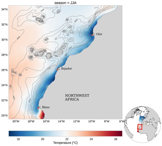
Figure 1.
Summer (June–August) climatology of SST (°C) across the Northwest African region. The main figure illustrates the coastal temperature pattern. Dashed grey contour lines denote the bathymetry, highlighting seafloor features associated with upwelling processes. The small globe in the bottom-right corner shows the IBI (Iberian–Biscay–Ireland) region from the Copernicus dataset, with the study area outlined in red to indicate its position relative to the larger domain.

Table 1.
Geographic coordinates of the area of study.
Differentiating marine and terrestrial cells is essential for model training and inference. To this end, a binary land–sea mask was calculated, as shown in Figure 2. A bathymetry-based mask was also generated using NOAA’s ETOPO model [47], providing depth information relevant for capturing nearshore variability. The bathymetric data were downscaled to match the grid resolution of the SST fields (see Figure 2). These masks supply physical context to the model and improve performance in regions characterized by strong topographic gradients.
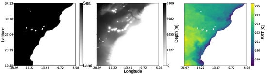
Figure 2.
Spatial fields over the Canary Islands region. (Left): Land–sea mask distinguishing ocean (black) from land (white). (Center): Bathymetry (in meters). (Right): Sea surface temperature (SST, in Kelvin) on 1 January 2018.
3.2. Graph Neural Network and Mesh Design
The predictive framework employs an encoder–processor–decoder architecture based on interaction networks [48]. Message passing is used to exchange information across the latent mesh and the observational grid. This design aligns with recent geophysical models such as GraphCast [43], Hi-LAM [44], and SeaCast [17], which demonstrate the flexibility of bipartite grid-to-mesh graph representations for data-driven climate forecasting. The model configuration used here isolates the role of mesh design and connectivity by holding hyperparameters and optimization choices constant across experiments.
Four mesh construction strategies were considered with the following configurations:
- Uniform Mesh with Crossing Edges (UC-mesh): Adapted from SeaCast, in this strategy, nodes lie on a regular orthogonal grid with up to eight connections, including diagonals. While this maximizes neighborhood density (Figure 3a), triangle intersections increase edge count and computational cost.
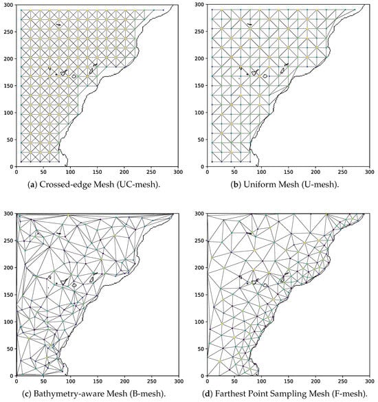 Figure 3. Comparison of the four mesh-generation strategies used in the experiments. All meshes contain 159 nodes but differ in node distribution and edge construction: UC-mesh includes 1090 edges arranged in a crossed-edge configuration, increasing connectivity via diagonals; U-mesh consists of 848 non-crossing edges derived from a Delaunay triangulation; B-mesh contains 906 edges generated from a bathymetry-weighted probabilistic sampling given by (2); F-mesh uses 858 edges connecting sampled nodes along the coastline through an adaptive redistribution strategy calculated from the bathymetry as in (3).
 - Uniform Mesh without Crossing Edges (U-mesh): In this second strategy, the position of nodes is also orthogonal as before, and edges are obtained through a Delaunay triangulation. In this case, edges do not cross, avoiding diagonal intersections (see Figure 3b). This reduces edge density while preserving spatial coverage. This configuration resembles the GraphCast model [43] in that edges do not cross, although it is a global atmospheric model that relies on an icosahedral mesh structure.
- Bathymetry-aware Mesh (B-mesh): In this case, node density is adapted to bathymetric variability, motivated by the greater bathymetry-driven SST gradients in coastal upwelling regions. Points are sampled according to probability distributions derived from normalized depth values. This improves spatial representation in coastal areas. Edges are also established using a Delaunay triangulation, as shown in Figure 3c. Based on the bathymetry () shown in Figure 2, we normalize the values in using min–max normalization:Nodes are placed based on the following probability function:and then, the distribution is used to place nodes non-uniformly. This strategy adapts better to the coast geometry, although it tends to concentrate a large number of nodes near the coast, leaving few points to represent extensive deeper areas.
- FPS Bathymetry-Based Mesh (F-mesh): This strategy aims to solve the drawbacks of the previous one, maintaining a more homogeneous node separation while still relying on the bathymetry. It covers the whole region by distributing the nodes adaptively using the Farthest Point Sampling (FPS) algorithm [49] and a more balanced distribution. To achieve this, we use the following function:where represents the value corresponding to the i-th percentile of the bathymetry, and denotes the interquartile range: that is, the difference between the third and first quartiles of the bathymetric distribution. We can then use the probability distribution to position the nodes in the mesh. This allows us to flexibly adjust the number of nodes in each area by varying the value of i, although we can also define a linear combination between two distributions as follows:where . If we choose to give greater weight to the coastal zone and to the deep ocean area, this relation allows us to flexibly balance the nodes between the coast and the ocean in a controlled manner. In our experiments, we used . This mesh configuration is shown in Figure 3d.
All meshes are preprocessed by removing land nodes and equipped with an encoder/decoder scheme following the hierarchical design of [17,44]. Three edge types define the connectivity: First, bidirectional mesh-to-mesh edges () link each mesh node () to its spatial neighbors; second, grid-to-mesh edges () connect every grid cell () to its k-nearest mesh nodes (); third, mesh-to-grid edges () close the cycle by projecting information back to the grid. Unlike earlier implementations, the hyperparameter k explicitly enforces a fixed number of encoder/decoder connections () per node (), guaranteeing consistent coverage across the domain.
3.3. Experimental Configuration
In this work, we designed two main experiments to assess the performance of the mesh configurations. On the one hand, we analyzed the influence of the connectivity between the grid and the mesh and its role in generating visible artifacts. On the other hand, we studied the influence of the number of nodes on the accuracy of the four strategies.
3.3.1. Experiment 1—Grid-to-Mesh Connectivity
The number of connections per node was varied between and across the four mesh types, yielding 20 different configurations. Each model was trained using the same number of epochs (150); the AdamW optimizer with , , and ; and a cosine-decay learning rate starting at . The loss function was the weighted mean squared error (), given by
where N is the number of nodes in the grid, is the binary land–sea mask defined in Section 3, and is the latitude-based weight given by [50]
which accounts for the varying size of the cells produced by the spherical coordinates, and s is the per-variable inverse variance of time differences. The ground truth value is given by , and the prediction is given by in each point i of the grid.
Table 2 shows the configuration of meshes used in this experiment, with the number of nodes and edges in each level. The number of nodes in the second layer of the F-mesh was increased because a node became isolated. This isolation was due to a combination of the morphology of the African coast and the operation of the farthest point sampling algorithm. By adding a single node, we achieved a fully connected mesh without compromising the comparison, as the total number of edges remains the same as in other configurations tested in this experiment.
Table 2.
Node and edge counts for the mesh configurations used in the grid-to-mesh connectivity experiment. To ensure fair comparison across topologies, all four mesh types (U-mesh, UC-mesh, B-mesh, and F-mesh) were constructed with approximately equal node counts at each resolution level. The F-mesh has one more node in Level 2 to avoid an isolated node and to maintain a similar number of edges.
Finally, a factorial analysis contrasted the main effects of mesh configuration, connectivity, and node density, as well as their interactions, on the target metrics. Differences in means and variances across experiments, confidence intervals, and post hoc tests were used to derive practical design criteria for robust grid-to-mesh coupling in geospatial prediction tasks.
3.3.2. Experiment 2—Node Density
For each mesh configuration, the node density was increased following a geometric progression with ratio , consistent with the refinement ratios suggested in the literature [51,52]. Fixed ratios simplify the control of spatial resolutions and error reduction, and using a golden-ratio increment offers a useful middle ground between typical refinement factors (≈1.5 to 2), giving meaningful resolution improvements without a sharp rise in computational cost. Alternative scaling schemes exist, but the golden ratio is favored for its balance between refinement detail and computational cost in adaptive physical simulations, where it reduces numerical discontinuities [53]. Similar advantages appear in geometric subdivision methods using for smoother multiresolution transitions [54], and theoretical work shows that golden-scale hierarchies match scale-distributed processes like turbulence [55], supporting -scaling as suitable for multiscale modeling.
All experiments maintained consistent vertical levels and the same number of nodes across mesh types. Mesh characteristics, including nodes and edges at hierarchical levels, are summarized in Table 3.
Table 3.
Node and edge counts per mesh configuration and hierarchical level. Each row corresponds to a target (Level 1 and Level 2) configuration, with node and edge counts reported for all four mesh types.
values are computed over the entire test set ad aggregated across the full date-time span (d) to obtain , where i stands for the flattened latitude–longitude grid location, and t denotes the lead time.
4. Results
This section analyzes the effects of grid-to-mesh connectivity, node density, and mesh topology on forecast accuracy and artifact formation. Unless otherwise stated, all models were trained under identical optimization settings and evaluated over the same temporal horizons: lead times spanning from 1 to 15 days, with global and per-tile of spatial gradients as primary metrics. Spatial diagnostics include error maps and automatic artifact detection based on the geometry of grid-to-mesh associations.
4.1. Influence of Grid-to-Mesh Connectivity
Table 4 summarizes mesh performance across all connectivity settings. B-mesh and F-mesh achieved the lowest (0.24 at and ), which improved the results of the structured meshes by nearly 30%. Its refinement according to seabed morphology concentrates resolution in coastal and high-gradient regions. However, the performance of the B-mesh is more sensitive to connection count, with a greater variability than any other mesh, as shown in Table 5 with , which indicates a strong dependency on tuning.
Table 4.
in Kelvin by mesh type and number of grid-to-mesh connections, k. The best value in each row is in bold.
Table 5.
Aggregate 15-lead-time statistics.
F-mesh, on the other hand, delivered the most consistent performance across connection counts. Its best result, with an of and connections, is nearly as good as B-mesh, but with less variance. Therefore, F-mesh offers a strong compromise between accuracy and robustness. Structured meshes (U-mesh and UC-mesh) perform similarly, with U-mesh slightly outperforming UC-mesh at their respective optima. Crossing edges exhibit the lowest variability but consistently higher mean , indicating limited adaptability compared with triangular meshes.
When aggregated over all five connectivity levels, F-mesh achieved the best mean (0.35 ± 0.06), followed by B-mesh (0.36 ± 0.08), U-mesh (0.39 ± 0.04), and UC-mesh (0.40 ± 0.02). These statistics (Table 5) highlight not only accuracy but also variability across connection settings.
These findings align with qualitative error maps for the B-mesh configuration, as shown in Figure 4. Low-connectivity settings () accentuate polygonal discontinuities and tessellation artifacts, likely explaining the poor performance of B-mesh with , while intermediate connectivity () reduces such artifacts and improves spatial coherence. At , error maps show signs of plateauing or mild regression, likely due to over-coupling and amplified message-passing interference.
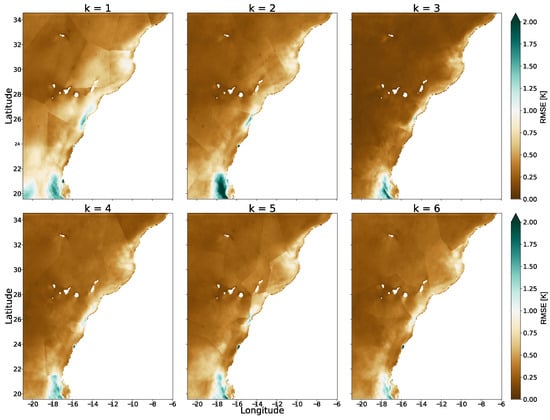
Figure 4.
Spatial distribution of at 15-day lead time for the B-mesh configuration under varying connectivity levels ( to 6). Lower connectivity () produces remarkable polygonal discontinuities and tessellation artifacts, particularly along coastal headlands, whereas intermediate connectivity () improves spatial coherence and suppresses mesh-induced distortions. The results for are included beyond the predefined range ) to verify that performance does not improve for a larger number of connections, further supporting as an optimal trade-off between coverage and over-coupling.
Figure 5 depicts the evolution of across forecast horizons for the B-mesh () and F-mesh () configurations. B-mesh with and F-mesh with consistently produce better results, while the errors of the F-mesh with and B-mesh with are higher. Differences are negligible in the first 4–5 days but increase progressively, reaching approximately 30% relative degradation by the 15th day, emphasizing the operational significance of topology–connectivity interactions.
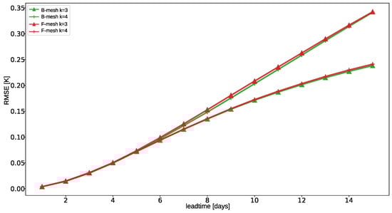
Figure 5.
Average as a function of forecast lead time for the four best-performing topology–connectivity configurations: B-mesh () and F-mesh (). Two distinct performance bands emerge beyond day 5, with B-mesh () and F-mesh () maintaining consistently lower error growth compared to B-mesh () and F-mesh (). Error differences widen progressively toward day 15, highlighting the sensitivity of long-range forecasts to mesh topology and connectivity order.
Table 6 shows the training and inference times for each mesh and connection count. Increasing k increases the number of and, therefore, memory and runtime. The computational cost increases linearly with the number of connections. During training, each additional edge adds on average between 6.6k and 6.8k seconds (≈1.8 h), corresponding to a relative increase of approximately 30% per edge compared to the case. In inference, the impact is substantially lower: around 570 s per edge (≈10 min), equivalent to a ∼25% increase.
Table 6.
Training and inference runtime (seconds) across mesh configurations and k values, measured on a remote server with 8× Quadro RTX 4000 GPUs and 8 GB of memory.
These results indicate that moderate connectivity (3–4 links per node) balances information flow and error control, while trimming excess edges reduces computational costs without performance loss. Bathymetry-based meshes, particularly F-mesh with mixed-sigmoid densification, yield smoother coastal errors, highlighting the importance of spatial adaptability. Forecast skills are mainly shaped by mesh topology after the first few days, and benefits become evident once resolution surpasses a critical threshold.
4.2. Influence of Bathymetry and Regime Imbalance
The analysis of distribution across bathymetric ranges, visualized through box plots and sample size histograms (Figure 6), reveals a critical physical regime imbalance. The upper histogram highlights a skewed data distribution, with the coastal domain (<) representing a significantly underrepresented minority compared to the open ocean. This scarcity correlates directly with model instability: The box plots in the shallow regime exhibit the largest interquartile ranges and whisker extensions, indicating maximum error variance and uncertainty. In contrast, the deep ocean regime (>) is characterized by compact boxes and stable medians, reflecting the GNN’s robust performance in the dominant, physically homogeneous class. These results suggest that the network’s optimization is biased towards the abundant deep-water samples, failing to generalize to the complex, data-scarce coastal dynamics where boundary effects and local variability prevail.
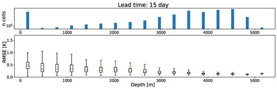
Figure 6.
Dependence of predictive performance on ocean depth for B-mesh () at 15-day forecasts. (Top panel): Histogram showing the frequency of grid cells across bathymetric ranges, illustrating the skewed distribution of data towards deep-water regions. (Bottom panel): Box plots of (K) versus depth (m). The plot reveals an inverse relationship between bathymetry and error variability: Coastal and continental shelf regions (0–1000 m) are characterized by high uncertainty and large error spread, whereas the abyssal plain (>3000 m) demonstrates robust model performance with compact error distributions.
4.3. Artifact Formation and Order-k Voronoi Effects
The spatial organization of the prediction error reveals a strong geometric imprint induced by the grid-to-mesh association. For the lowest connectivity (), the resulting partition closely resembles a first-order Voronoi diagram: Each mesh node defines a convex region, and the associated boundaries emerge where the Euclidean distance of two nodes is equal. The discontinuities in the field align with these borders, forming sharp, polygonal divisions across the domain (Figure 7). In this regime, tile boundaries are simple and coherent, and the geometry is dominated by the distance-based isolation of individual nodes.
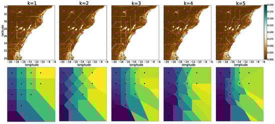
Figure 7.
Spatial gradients at 15-day lead time highlight deterministic tiling artifacts imposed by the grid-to-mesh connectivity (U-mesh). Although the polygonal discontinuities are already present in the maps, the |∇RMSE| representation makes the tile boundaries sharply visible. Magenta color points denote mesh node positions over the spatial domain. Top panels show the empirical gradient fields for different k settings, while bottom panels display analytically generated order-k Voronoi partitions using the same neighbor rule, reproducing the same geometry. This confirms that at longer lead times, the error field is governed by the tessellation induced by the connectivity mechanism rather than stochastic model behavior.
This observed geometric structure is not incidental but arises because the underlying grid-to-mesh coupling mechanism is mathematically equivalent to generating an order-k Voronoi diagram [56]. The formulation begins by defining the total number of mesh nodes as . The association mechanism, often implemented as the spatial distance (e.g., KD-tree search), identifies a generator subset for every grid node . This subset consists of the mesh nodes closest to . Crucially, k represents the fixed number of grid-to-mesh/mesh-to-grid connections () per node. The set of all possible unique generator subsets is , where . Each distinct subset is explicitly defined as containing k mesh nodes, .
Each subset defines a unique region known as an Order-k Voronoi Polygon, (Equation (7)). This specific polygon, , represents one of the distinct polygonal error regions (artifacts) observed in the prediction maps. It encompasses all grid nodes that satisfy the following geometrical constraint:
The full set of these polygons, , is the induced order-k Voronoi diagram. This complete tessellation, which reflects deterministic changes in neighbor sets, constitutes the spatial organization of the prediction error field. In the autoregressive GNN, this partitioning ensures that each Voronoi tile behaves as a semi-independent predictor, causing errors to accumulate with distinct, tile-specific growth slopes over long lead times.
This equivalence (Equation (8)) holds because the membership of a grid node () in an Order-k Voronoi polygon () is entirely determined by its set of k nearest neighbors . This relationship is formally proven by biconditional equivalence:
where is the function that returns the k-nearest neighbor set () of . Since each polygon () is uniquely defined by a single k-element generator subset (), the double inclusion is fulfilled: When the neighbor set of coincides with this generator subset, the point satisfies the defining condition of the corresponding order-k Voronoi polygon; when it differs, it necessarily lies outside its boundaries. Thus, the biconditional relationship arises directly from the definition of the order-k diagram, where region boundaries occur precisely at locations where its associated changes.
As connectivity increases, the geometry of the induced partitions undergoes a qualitative shift. Instead of single-node dominance, each region is defined by overlapping neighborhoods of multiple mesh nodes. The resulting tiles lose convexity, become irregular, and exhibit fragmentation or elongation in certain areas. This increase in geometric complexity is spatially heterogeneous: Some zones retain simple structures, while others subdivide into non-convex or highly anisotropic shapes. The average tile area decreases with higher k, but this refinement does not translate into smoother error fields. Instead, the boundaries persist and frequently intensify, especially at vertices where three or more tiles converge, which act as localized amplification points for error growth under autoregressive prediction.
To confirm the geometric origin of these patterns, the connectivity mechanism was replicated using a synthetic mesh placed over a domain (Figure 8). Each grid point was assigned its k-nearest neighbors via the same KD-tree-based search used in the encoder–decoder forecasting framework. The resulting partitions reproduced the theoretical structure of order-k Voronoi diagrams described in the analytical literature [57], matching the reference formulation precisely. Applying the same procedure to the U-mesh configuration from to 5 yielded a tessellation with boundaries replicating those artifacts, validating that the spatial organization of the gradients is a direct consequence of the k-NN association (Figure 7). The discontinuities in the error are therefore not incidental: they reflect deterministic changes in neighbor sets across partition interfaces.
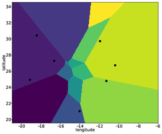
Figure 8.
Reproduction of the order-3 Voronoi diagram from [57], generated using the same site configuration. In our framework, applying a grid-to-mesh association with nearest neighbors via KD-tree yields the same partition geometry, demonstrating that the connectivity mechanism is mathematically equivalent to an order-3 Voronoi construction. This validates that the polygonal artifacts observed in the || fields arise directly from the deterministic tessellation induced by the k-NN association rule. Distinct colors represent different Voronoi regions, each defined by a unique set of k-nearest neighbors.
Coastal boundaries truncate tiles and remove candidate neighbors, creating smaller and more irregular cells than in offshore regions. Euclidean distances in latitude–longitude space further introduce directional bias, particularly along the north–south axis, distorting partition geometries. These geometric distortions interact with strong coastal SST gradients and localized heterogeneity, amplifying error accumulation. To systematically capture these effects, we introduce Error Analysis by Spatial Tessellation in Appendix A, a diagnostic framework that partitions the domain into tiles and tracks the evolution of forecast errors within each cell. Histograms of per-tile reveal heavy-tailed behavior near the coast (Figure A2), while offshore tiles display more symmetric distributions. The tile-averaged grows approximately linearly with lead time (Figure A3), but growth rates vary sharply across space, with the steepest slopes concentrated along coastal bands.
Increasing k does not eliminate these discontinuities. Although higher connectivity reduces individual tile size (Figure 7), it simultaneously increases fragmentation, irregularity, and the frequency of intersections. The transitions between neighbor sets remain discrete, preserving the geometric basis of the discontinuities. gradients continue to align with the tile boundaries, and vertices formed by multi-tile intersections become preferential sites for accelerated error propagation. The persistence of these structures indicates that artifacts arise from the intrinsic geometry of the k-NN mechanism rather than from insufficient neighbor node count or model performance.
The spatial structure of the is dictated by the grid-to-mesh association, where tile geometry depends on connectivity and node placement. In autoregressive settings, each tile acts as a semi-independent predictor with distinct error dynamics (Figure A3), producing spatial–temporal heterogeneity. Artifact formation arises from the equivalence between connectivity rules and a Voronoi partition, implying that mitigation requires altering the association geometry rather than merely increasing connectivity.
4.4. Influence of the Number of Mesh Nodes
Across the four mesh configurations, trajectories remain nearly identical during the first four to five lead-time days, regardless of node count, as can be observed in Figure 9a. At these short horizons, forecast accuracy is primarily governed by initial observational states and the intrinsic predictive skill of the model, leaving mesh topology with negligible influence.
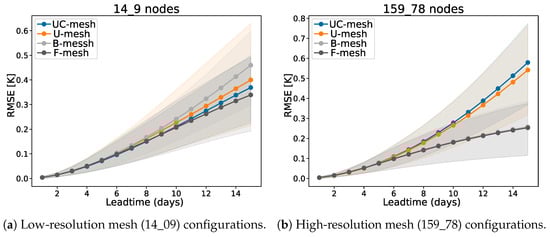
Figure 9.
Forecast trajectories with associated uncertainty across prediction horizons for different mesh configurations under two levels of spatial resolution. Solid lines represent the mean (dressed ), while shaded regions denote the 66% confidence intervals. (a) When the number of mesh nodes is low (14_9), all four configurations exhibit nearly parallel error evolution, with only minor divergence emerging after day 5. The substantial overlap of the confidence intervals confirms that the minor divergence observed after day 5 is not statistically significant. The limited spatial resolution constrains information propagation, suppressing the advantages of unstructured meshes. (b) At higher node density (159_78), the separation beyond day 5 becomes much more pronounced. Unstructured meshes (F-mesh and B-mesh) sustain lower error growth, with confidence bounds distinct from the structured baselines, indicating superior long-range predictive skill once spatial resolution is sufficient to exploit their adaptive placement.
To rigorously quantify forecast uncertainty and validate performance differences, the posterior distribution of the was modeled using Bayesian Neural Fields [58], generating a probabilistic ensemble of samples. We applied a mean bias correction (“Error Dressing”; [59]) and evaluated comparative performance using the distribution of paired differences (), following [60] to account for temporal correlation. Significance was determined via a Zero-Inclusion Criterion on the 66% credibility intervals, as described by [61].
Applying this framework to the high-density node configuration (Figure 9b) reveals a statistically significant divergence from day six onward. While structured meshes (U-mesh and UC-mesh) show a steep increase in error, F-mesh and B-mesh sustain lower error growth with paired difference intervals that consistently exclude zero. This confirms the existence of a temporal activation window: beyond day 6, error accumulation due to autoregressive structural artifacts is significantly mitigated by the adaptive geometry of unstructured meshes.
Conversely, when node counts are reduced, these statistical distinctions vanish across the entire prediction horizon (Figure 9a). The 66% credibility intervals for the differences largely overlap with zero, indicating that insufficient spatial resolution suppresses topology effects. These results identify a spatial resolution threshold: below a critical node density (e.g., 34 or 20 nodes), representational capacity becomes the dominant limiting factor, rendering the choice between structured and unstructured designs statistically negligible.
A secondary observation relates to the role of diagonal crossing edges in the UC-mesh. Configurations without crossing edges (U-mesh) occasionally show slightly more stable trajectories than those with intersecting connections (UC-mesh), suggesting that excessive edge proliferation may compound long-range error growth. However, this effect remains secondary to the broader distinction between structured and unstructured designs.
At the seventh-day lead time, all configurations show marginal differences (Figure 10a), with structured meshes sometimes presenting slightly lower than unstructured ones. The error curves remain nearly flat across resolutions, reinforcing the dominance of initial conditions at very short horizons.
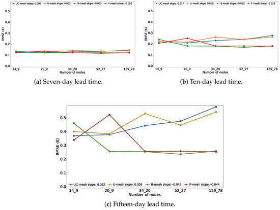
Figure 10.
Comparison of RMSEs across node densities at different lead times. While all configurations behave similarly at seven lead times, structured meshes progressively degrade with higher node counts at ten and fifteen lead times. In contrast, unstructured layouts exhibit more stable or improving error performance as resolution increases.
By the tenth day lead time, a transitional regime emerges. Structured configurations begin to show a gradual increase in with higher node counts (Figure 10b), while the unstructured meshes remain stable or even improve modestly, particularly in the bathymetric layout. This suggests that once the constraint of the initial state weakens, topology-sensitive designs can better capture underlying SST variability.
At the fifteen-day horizon (Figure 10c), the divergence becomes pronounced. Structured meshes degrade substantially with increasing node count—especially in crossing-edge cases—whereas unstructured designs either maintain or reduce levels as resolution increases. This inversion underscores that unstructured strategies not only accommodate spatial heterogeneity more effectively but also scale more robustly with forecast length.
Increasing node count alone does not guarantee improved forecast accuracy. At higher spatial resolutions, differences between mesh families become apparent only beyond day five. Here, unstructured meshes consistently outperform structured ones (Figure 10c), demonstrating that the spatial organization and connectivity—not raw node count—determine whether added resolution yields meaningful gains.
Notably, the B-mesh is highly effective at higher resolutions but performs comparatively worse at low node densities, indicating that adaptive placement requires a minimum number of nodes to operate effectively. F-mesh exhibits an intermediate behavior but similarly loses advantage when spatial capacity is limited.
Spatial analyses of squared-error fields at day 15 reveal clear contrasts among mesh families as resolution increases. In structured meshes, artifacts remain visible even at higher node counts (Figure 11a), although their footprint shrinks. Coastal regions consistently emerge as hotspots of error due to the rigid and uniform connectivity of these grids, which limits their ability to represent strong nearshore gradients.
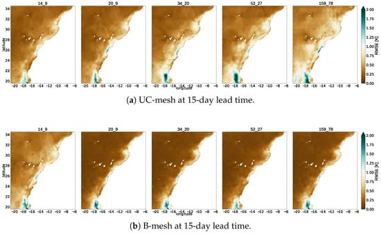
Figure 11.
Spatial distribution of at 15-day lead time across increasing node densities for UC-mesh and B-mesh configurations. Structured grids exhibit persistent polygonal tessellation artifacts and concentrated coastal errors even at higher resolutions, reflecting limited adaptability to sharp shoreline gradients. In contrast, the unstructured B-mesh produces smoother and more coherent error fields, notably attenuating nearshore and constraining offshore error propagation due to morphology-aware node placement.
Unstructured configurations exhibit smoother and more coherent error fields (Figure 11b), with far fewer discretization artifacts. The B-mesh shows the clearest advantage: Errors near the coast are reduced, and offshore propagation is constrained more effectively than in structured designs. Because node placement reflects underlying morphology, transitions between coastal and open-ocean regions are better resolved, attenuating artificial discontinuities.
F-mesh shows intermediate behavior. They benefit from increased resolution and lack of rigid cell imprinting, but they do not suppress coastal error growth as consistently as the bathymetric layout. Across lead times, unstructured meshes modulate not only the magnitude but also the spatial evolution of . At higher node densities—particularly in the B-mesh configuration—error growth remains more localized and physically coherent, aligning with the statistical trends observed in the curves.
5. Discussion
A decisive step in interpreting these results is the geometric diagnosis of artifacts. Geometric discretization schemes, such as Voronoi diagrams, can either introduce or reveal heterogeneity. While such structures may be advantageous in physics-based numerical simulations [62], in autoregressive GNN-based models, they can become an unintended source of structured error. The grid-to-mesh association induces partitions that are algebraically equivalent to order-k Voronoi diagrams [57]; tile boundaries in these diagrams align with the polygonal error patterns observed in the maps. This explains the persistence of artifacts in autoregressive settings: Each tile behaves as a partially isolated predictor with its own error trajectory (Figure A3), producing approximately linear per-tile slopes that diverge over lead time. Hence, the core issue is not only error magnitude but the spatial–temporal heterogeneity of error accumulation determined by association geometry.
While geometric analogies with traditional discretization methods such as the finite element method are conceptually relevant—both involve mesh-induced partitions that shape error patterns—the present work does not aim to establish a formal numerical equivalence or perform a horizontal comparison with FEM. Our focus is instead on diagnosing artifact formation within GNN-based grid–mesh associations.
Beyond the geometric artifacts discussed above, a secondary source of error arises from the unequal distribution of training data across depth regimes. Regardless of the mesh topology, the error magnitude intensifies significantly in nearshore zones. As shown in Figure 6, the error profile reveals a bottleneck in shallow waters that is distinct from the tessellation patterns: The model exhibits its highest uncertainty in these regions due to a severe class imbalance between the dominant deep-ocean samples and the narrow coastal margins. This class imbalance is consistent with the inherent morphology of the ocean floor. The spatial extent of abyssal plains (typically ranging from 3000 to 6000 m) vastly exceeds that of continental shelves ( m) and slopes, which exist only as narrow transitional margins bordering the landmasses. Consequently, the dominance of deep-water samples is not a sampling artifact, but a direct reflection of the natural bathymetric distribution within the study area.
Some studies suggest a direct trade-off between accuracy and node count [63], assuming that denser meshes typically lead to lower error, reinforcing the idea that more nodes yield better accuracy. However, our results bring into question this perspective by clarifying why indiscriminate increases in k connections or node count are insufficient. While unstructured meshes (F-mesh and B-mesh) coupled with intermediate number of connections () reduce artifact incidence and long-horizon , the effect is topology-dependent: In highly structured lattices (U-mesh and UC-mesh), increasing the number of mesh nodes reduces the area associated with each node—meaning that fewer grid points contribute information to each mesh node. Because these lattices have uniform edge lengths, the edge embeddings become highly redundant, providing limited new information to the learning process.
Higher k increases training costs and memory/latency, while overly dense structured meshes can degrade performance due to reduced input diversity and geometric redundancy. Our results show that a careful hyperparameter selection preserves accuracy while reducing total computational cost, using a intermediate k. In practice, latent mesh capacity should be concentrated in coastal zones and regions with steep error gradients, where capturing finer-scale structures is essential for improving forecast accuracy.
Conceptually, the results establish a direct link between artifact morphology and discrete computational geometry: When the association mechanism is equivalent to an order-k Voronoi diagram, partition properties predict where and how artifacts arise. This reproduces prior empirical observations [12,13] (e.g., polygonal seams, tile discontinuities) and provides a predictive analytical tool to guide design choices.
In oceanographic forecasting with GNNs, the connectivity between the observational grid and the latent mesh (encoder/decoder) must be treated as a tunable design hyperparameter rather than a fixed architectural choice. Unlike other domains where this component may be incidental or predefined [17,44], here, the mesh’s spatial density, distribution, and connectivity to the observational grid directly control prediction accuracy and artifact behavior. Tailored interventions, such as redistributing nodes in sensitive regions, as demonstrated in other works [64,65]; adjusting connectivity by weighting edges according to their angular span in the Voronoi diagram [63]; or removing redundant crossings, can suppress discontinuities without excessive computation. Bathymetry-aware layouts generally enhance coastal consistency, whereas regular lattices with diagonal links tend to amplify seams.
Three avenues emerge for advancing oceanographic GNNs. The association between grid and mesh should move beyond rigid order-k matching toward stochastic or affinity-weighted connections, diffuse neighborhoods, or spatial kernels that soften partitions. Local artifact control can be achieved through tile-level corrections informed by trends, using adaptive latent meshes, mesh-to-grid residual connections, or even non-autoregressive and hybrid decoders to reduce temporal heterogeneity. Decisions on increasing k or node density should be guided by explicit temporal and spatial statistics and validated across regions, variables (e.g., winds, salinity), and resolutions to assess generality. Statistical diagnostics that uses our proposed Error Analysis by Spatial Tessellation (Appendix A) could ultimately act as inference-time controllers, triggering adaptive responses before coherence breaks down. Together, these steps outline both a geometric perspective and a concrete toolkit for anticipating and suppressing artifacts before they erode physical compliance and operational value.
This study does not yet account for the seasonal dependence of SST prediction errors, nor does it assess model behavior across contrasting oceanographic regimes beyond the Canary Islands–Northwest Africa region. These two aspects—seasonal robustness and cross-regional generalization—remain important limitations of the present work and will be the focus of our future research.
6. Conclusions
This work identifies the geometry of the grid-to-mesh coupling as the primary driver of artifacts that undermine geospatial forecast quality. The association mechanism is algebraically equivalent to an order-k Voronoi partition, so each tile acts as a partially isolated predictor for which its errors accumulate with approximately linear, tile-specific slopes. Consequently, indiscriminately increasing connectivity or node count is insufficient; effective mitigation requires controlling the coupling geometry. In practice, intermediate connectivity () and bathymetry-aware configurations reduce polygonal seams and long-horizon , especially when coupling emphasizes smooth information exchange across tile boundaries.
Operational recommendations follow a cost–benefit logic. Latent node capacity should be allocated strategically, prioritizing high coastal SST gradients (upwelling zones) and regions with steep per-tile slopes rather than increasing the number of nodes indiscriminately. In structured mesh configurations, excessive node proliferation can, in fact, degrade performance, underscoring that connectivity must be scaled in line with available training time and memory resources. The k parameter should be treated as a critical methodological choice, guided by spatial error diagnostics such as Error Analysis by Spatial Tessellation.
Future work should explore more flexible association mechanisms to soften tessellation boundaries and reduce interface artifacts. Additional directions include localized correction strategies informed by spatial error signals, alternative decoding schemes that mitigate temporal drift, broader validation across domains and variables, and principled analyses linking mesh connectivity and sampling density to artifact behavior.
Author Contributions
Conceptualization, G.A.C.-L., J.G.R. and J.S.; methodology, G.A.C.-L. and J.S.; software, J.G.R. and G.A.C.-L.; validation, G.A.C.-L.; formal analysis, G.A.C.-L., J.G.R. and J.S.; investigation, J.G.R. and G.A.C.-L.; resources, J.S.; data curation, J.G.R.; writing—original draft preparation, G.A.C.-L. and J.G.R.; writing—review and editing, G.A.C.-L., J.G.R. and J.S.; visualization, G.A.C.-L.; supervision, J.S.; funding acquisition, J.S. and Á.R.-S. All authors have read and agreed to the published version of this manuscript.
Funding
This research received institutional support from the Instituto Universitario de Investigación en Acuicultura Sostenible y Ecosistemas Marinos (ECOAQUA) and the Centro de Tecnologías de la Imagen (CTIM), but no external funding was received.
Institutional Review Board Statement
Not applicable.
Informed Consent Statement
Not applicable.
Data Availability Statement
The sea surface temperature (SST) data used in this study were obtained from the Copernicus Marine Service Program (product name: SST_reanalysis; available at https://data.marine.copernicus.eu/product/SST_ATL_SST_L4_REP_OBSERVATIONS_010_026 (accessed on 26 June 2025)). The wind reanalysis data at 10 m above the surface were retrieved from the European Centre for Medium-Range Weather Forecasts (ECMWF) through the ERA5 dataset (available at https://www.ecmwf.int/en/forecasts/datasets/reanalysis-datasets/era5 (accessed on 26 June 2025)). Bathymetric data were sourced from NOAA’s ETOPO Global Relief Model (https://www.ncei.noaa.gov/products/etopo-global-relief-model (accessed on 26 June 2025)). All datasets are publicly accessible under their respective usage licenses. The full source code used to train the models and reproduce all experiments will be made publicly available at the following repository: https://github.com/gacuervol/grid2mesh-voronoi-artifacts.git (accessed on 3 December 2025)).
Acknowledgments
The authors would like to thank the technical teams at ECOAQUA and CTIM for computational support during model training and experimentation. The authors also acknowledge the Copernicus Marine Service, ECMWF, and NOAA for providing open-access oceanographic datasets used throughout this study. During the preparation of this manuscript, the authors used GPT-4o model (accessed on 15 October 2025), Gemini 1.5 Pro model (accessed on 15 October 2025) and Perplexity AI, https://www.perplexity.ai, (accessed on 15 October 2025) for language polishing, grammar refinement, and the restructuring of selected paragraphs for clarity. The authors have reviewed and edited all generated content and take full responsibility for the final version of this publication.
Conflicts of Interest
The authors declare no conflicts of interest.
Abbreviations
The following abbreviations are used in this manuscript:
| GNN | Graph Neural Network; |
| FPS | Farthest Point Sampling; |
| RMSE | Root Mean Squared Error; |
| WMSE | Weighted Mean Squared Error; |
| SST | Sea Surface Temperature. |
Appendix A. Error Analysis by Spatial Tessellation
The discontinuities observed in the spatial fields follow the boundaries of the order-k Voronoi-type tessellation generated by the k-NN connectivity (Figure A1a). Nearshore cells are truncated by the coastline and exhibit higher environmental gradients, resulting in systematically larger and more irregular prediction errors.
Per-cell distributions reflect this contrast: coastal tiles display skewed or heavy-tailed histograms, while offshore cells tend toward near-Gaussian behavior (Figure A2).
Alongside -based metrics, the spatial error was assessed using gradient comparisons per-tile :
where the subscript denotes the tile index, and the bar stands for the initial spatial averaging over all points within that tile, thus leaving the function exclusively dependent on lead time t. The final aggregated metric is then computed by taking the derivative with respect to the lead time, , of this spatially averaged function for each tile, which yields the instantaneous slope, and subsequently calculating the arithmetic mean of these slopes across all tiles.

Figure A1.
Spatial (a) and error-growth (b) diagnostics of asymmetry between coastal and offshore regions. Panel (a) shows U-mesh () spatial artifacts aligned with Voronoi tessellation boundaries, where tessellation cells near the coast are distorted by land proximity. Panel (b) quantifies this effect: coastal cells exhibit higher mean , larger variability, and steeper growth across lead times compared to offshore regions. Colors in the inset of (b) encode the slope, indicating faster error accumulation in coastal areas.

Figure A2.
U-mesh () 15-day lead-time histograms by tessellation cell: coastal versus offshore behavior.
The temporal evolution of mean per cell increases approximately linearly with lead time (Figure A3); however, the slopes vary markedly across the tessellation, with the steepest growth confined to coastal regions (Figure A1b).

Figure A3.
Evolution of U-mesh () across forecast lead times for each tessellation cell. Slopes are estimated using linear regression.
Spatial error organization arises from the joint effect of connectivity geometry and coastal constraint (Figure A1a,b), leading to a marked contrast between nearshore and offshore error regimes.
References
- Gattuso, J.P.; Magnan, A.K.; Bopp, L.; Cheung, W.W.; Duarte, C.M.; Hinkel, J.; Mcleod, E.; Micheli, F.; Oschlies, A.; Williamson, P.; et al. Ocean Solutions to Address Climate Change and Its Effects on Marine Ecosystems. Front. Mar. Sci. 2018, 5, 337. [Google Scholar] [CrossRef]
- Levin, L.A.; Brito-Morales, I.; Schoeman, D.S.; Hellberg, M.E.; Hemery, L.G.; Kudela, R.M.; Meinvielle, M.; Morato, T.; Sogin, M.L.; Thomas, C.J.; et al. Climate velocity reveals increasing exposure of deep-ocean biodiversity to future warming. Nat. Clim. Change 2020, 10, 576–584. [Google Scholar] [CrossRef]
- IPCC. IPCC Special Report on the Ocean and Cryosphere in a Changing Climate; Pörtner, H.-O., Roberts, D.C., Masson-Delmotte, V., Zhai, P., Tignor, M., Poloczanska, E., Mintenbeck, K., Alegría, A., Nicolai, M., Okem, A., et al., Eds.; Technical Report; Intergovernmental Panel on Climate Change: Geneva, Switzerland, 2019. [Google Scholar]
- Blayo, E.; Debreu, L. Adaptive Mesh Refinement for Finite-Difference Ocean Models: First Experiments. J. Phys. Oceanogr. 1999, 29, 1239–1250. [Google Scholar] [CrossRef]
- Pain, C.C.; Piggott, M.D.; Goddard, A.J.; Fang, F.; Gorman, G.J.; Marshall, D.P.; Eaton, M.D.; Power, P.W.; de Oliveira, C.R.M. Optimisation based bathymetry approximation through constrained unstructured mesh adaptivity. Ocean Eng. 2005, 32, 1624–1654. [Google Scholar] [CrossRef]
- Zhang, Q.; Wang, H.; Dong, J.; Zhong, G.; Sun, X. Applications of deep learning in physical oceanography: A comprehensive review. Front. Mar. Sci. 2024, 11, 1396322. [Google Scholar] [CrossRef]
- Bolton, T.; Zanna, L. Applications of Deep Learning to Ocean Data Inference and Subgrid Parameterization. J. Adv. Model. Earth Syst. 2019, 11, 376–399. [Google Scholar] [CrossRef]
- Fablet, R.; Febvre, Q.; Drumetz, L.; Rousseau, F. Recent Developments in Artificial Intelligence in Oceanography. Ocean-Land-Atmos. Res. 2022, 2022, 9870950. [Google Scholar] [CrossRef]
- Wang, X.; Guo, X.; Zhang, H.; Luo, J.; Jin, W.; Wang, X. A three-dimensional dynamic spatial-temporal graph neural network for ocean temperature field prediction. Eng. Appl. Artif. Intell. 2025, 127, 107304. [Google Scholar] [CrossRef]
- Liang, S.; Zhao, A.; Qin, M.; Hu, L.; Wu, S.; Du, Z.; Liu, R. A Graph Memory Neural Network for Sea Surface Temperature Prediction. Remote Sens. 2023, 15, 3539. [Google Scholar] [CrossRef]
- Reyes, J.G.; Cuervo-Londoño, G.A.; Sánchez, J. Adaptive Meshes in Graph Neural Networks for Predicting Sea Surface Temperature Through Remote Sensing. In Proceedings of the Computer Analysis of Images and Patterns; Castrillón-Santana, M., Travieso-González, C.M., Deniz Suarez, O., Freire-Obregón, D., Hernández-Sosa, D., Lorenzo-Navarro, J., Santana, O.J., Eds.; Springer: Cham, Switzerland, 2025; pp. 361–372. [Google Scholar]
- Cuervo-Londoño, G.A.; Sánchez, J.; Rodríguez-Santana, A. Deep Learning Weather Models for Subregional Ocean Forecasting: A Case Study on the Canary Current Upwelling System; Technical Report; Cornell University: Ithaca, NY, USA, 2025. [Google Scholar] [CrossRef]
- Cuervo-Londoño, G.A.; Sánchez, J.; Rodríguez-Santana, Á. Forecasting Sea Surface Temperature from Satellite Images with Graph Neural Networks. In Proceedings of the Computer Analysis of Images and Patterns. CAIP 2025; Castrillón-Santana, M., Travieso-González, C.M., Deniz Suarez, O., Freire-Obregón, D., Hernández-Sosa, D., Lorenzo-Navarro, J., Santana, O.J., Eds.; Lecture Notes in Computer Science. Springer: Cham, Switzerland, 2025; Volume 15622, pp. 329–339. [Google Scholar] [CrossRef]
- Chassignet, E.P.; Hurlburt, H.E.; Smedstad, O.M.; Halliwell, G.R.; Hogan, P.J.; Wallcraft, A.J.; Baraille, R.; Bleck, R. The HYCOM (HYbrid Coordinate Ocean Model) data assimilative system. J. Mar. Syst. 2007, 65, 60–83. [Google Scholar] [CrossRef]
- Racault, M.F.; Le Quéré, C.; Buitenhuis, E.; Sathyendranath, S.; Platt, T. Phytoplankton phenology in the global ocean. Ecol. Indic. 2012, 14, 152–163. [Google Scholar] [CrossRef]
- European Union—Copernicus. Sobre Copernicus. 2025. Available online: https://www.copernicus.eu/es/sobre-copernicus (accessed on 6 May 2025).
- Holmberg, D.; Clementi, E.; Roos, T. Regional Ocean Forecasting with Hierarchical Graph Neural Networks. arXiv 2024, arXiv:2410.11807. [Google Scholar] [CrossRef]
- Robinson, A.R.; Lermusiaux, P.F. Ocean forecasting: Conceptual Basis and Applications; Springer: Berlin/Heidelberg, Germany, 2002. [Google Scholar] [CrossRef]
- Reichstein, M.; Camps-Valls, G.; Stevens, B.; Jung, M.; Denzler, J.; Carvalhais, N. Deep learning and process understanding for data-driven Earth system science. Nature 2019, 566, 195–204. [Google Scholar] [CrossRef]
- Zhao, X.; Qi, J.; Yu, Y.; Zhou, L. Deep learning for ocean temperature forecasting: A survey. Intell. Mar. Technol. Syst. 2024, 2, 28. [Google Scholar] [CrossRef]
- Sun, T.; Feng, Y.; Li, C.; Zhang, X. High Precision Sea Surface Temperature Prediction of Long Period and Large Area in the Indian Ocean Based on the Temporal Convolutional Network and Internet of Things. Sensors 2022, 22, 1636. [Google Scholar] [CrossRef]
- Mao, K.; Liu, C.; Zhang, S.; Gao, F. Reconstructing Ocean Subsurface Temperature and Salinity from Sea Surface Information Based on Dual Path Convolutional Neural Networks. J. Mar. Sci. Eng. 2023, 11, 1030. [Google Scholar] [CrossRef]
- Feng, M.; Boschetti, F.; Ling, F.; Zhang, X.; Hartog, J.R.; Akhtar, M.; Shi, L.; Gardner, B.; Luo, J.J.; Hobday, A.J. Predictability of sea surface temperature anomalies at the eastern pole of the Indian Ocean Dipole—Using a convolutional neural network model. Front. Clim. 2022, 4, 925068. [Google Scholar] [CrossRef]
- Mu, B.; Qin, B.; Yuan, S. Multi-scale downscaling with Bayesian convolution network for ENSO SST pattern. In Proceedings of the 2020 5th International Conference on Electromechanical Control Technology and Transportation (ICECTT), Nanchang, China, 15–17 May 2020; pp. 359–362. [Google Scholar] [CrossRef]
- Xie, B.; Qi, J.; Yang, S.; Sun, G.; Feng, Z.; Yin, B.; Wang, W. Sea Surface Temperature and Marine Heat Wave Predictions in the South China Sea: A 3D U-Net Deep Learning Model Integrating Multi-Source Data. Atmosphere 2024, 15, 86. [Google Scholar] [CrossRef]
- Zhang, S.Y.; Yang, Y.Z.; Xie, K.W.; Gao, J.H.; Zhang, Z.Y.; Niu, Q.R. Spatial-Temporal Siamese Convolutional Neural Network for Subsurface Temperature Reconstruction. IEEE Trans. Geosci. Remote Sens. 2024, 62, 1–16. [Google Scholar] [CrossRef]
- Zuo, X.; Zhou, X.; Guo, D.; Li, S.; Liu, S.; Xu, C. Ocean Temperature Prediction Based on Stereo Spatial and Temporal 4-D Convolution Model. IEEE Geosci. Remote Sens. Lett. 2022, 19, 1–5. [Google Scholar] [CrossRef]
- Izumi, T.; Amagasaki, M.; Ishida, K.; Kiyama, M. Super-Resolution of Sea Surface Temperature with Convolutional Neural Network- and Generative Adversarial Network-Based Methods. J. Water Clim. Change 2022, 13, 1673–1683. [Google Scholar] [CrossRef]
- Hochreiter, S.; Schmidhuber, J. Long Short-Term Memory. Neural Comput. 1997, 9, 1735–1780. [Google Scholar] [CrossRef]
- Cho, K.; van Merrienboer, B.; Gulcehre, C.; Bahdanau, D.; Bougares, F.; Schwenk, H.; Bengio, Y. Learning Phrase Representations Using RNN Encoder-Decoder for Statistical Machine Translation; Technical Report; Cornell University: Ithaca, NY, USA, 2014. [Google Scholar]
- Shi, X.; Chen, Z.; Wang, H.; Yeung, D.Y.; Wong, W.K.; Woo, W.C. Convolutional LSTM Network: A Machine Learning Approach for Precipitation Nowcasting; Technical Report; Cornell University: Ithaca, NY, USA, 2015. [Google Scholar]
- Zhang, K.; Geng, X.; Yan, X.H. Prediction of 3-D Ocean Temperature by Multilayer Convolutional LSTM. IEEE Geosci. Remote Sens. Lett. 2020, 17, 1303–1307. [Google Scholar] [CrossRef]
- Yang, Y.; Dong, J.; Sun, X.; Lima, E.; Mu, Q.; Wang, X. A CFCC-LSTM Model for Sea Surface Temperature Prediction. IEEE Geosci. Remote Sens. Lett. 2018, 15, 207–211. [Google Scholar] [CrossRef]
- Yu, X.; Shi, S.; Xu, L.; Liu, Y.; Miao, Q.S.; Sun, M. A novel method for sea surface temperature prediction based on deep learning. Math. Probl. Eng. 2020, 2020, 6387173. [Google Scholar] [CrossRef]
- Lin, Y.D.; Zhong, G.Q. A multi-channel LSTM model for sea surface temperature prediction. J. Phys. Conf. Ser. 2021, 1880, 012029. [Google Scholar] [CrossRef]
- Hou, S.; Li, W.; Liu, T.; Zhou, S.; Guan, J.; Qin, R.; Wang, Z. D2CL: A Dense Dilated Convolutional LSTM Model for Sea Surface Temperature Prediction. IEEE J. Sel. Top. Appl. Earth Obs. Remote Sens. 2021, 14, 12514–12523. [Google Scholar] [CrossRef]
- Pan, X.; Jiang, T.; Sun, W.; Xie, J.; Wu, P.; Zhang, Z.; Cui, T. Effective Attention Model for Global Sea Surface Temperature Prediction. Expert Syst. Appl. 2024, 254, 124411. [Google Scholar] [CrossRef]
- Liu, X.; Wilson, T.; Tan, P.N.; Luo, L. Hierarchical LSTM Framework for Long-Term Sea Surface Temperature Forecasting. In Proceedings of the 2019 IEEE International Conference on Data Science and Advanced Analytics (DSAA), Washington, DC, USA, 5–8 October 2019; pp. 41–50. [Google Scholar] [CrossRef]
- Xie, J.; Ouyang, J.; Zhang, J.; Jin, B.; Shi, S.; Xu, L. An Evolving Sea Surface Temperature Predicting Method Based on Multidimensional Spatiotemporal Influences. IEEE Geosci. Remote Sens. Lett. 2021, 19, 1–5. [Google Scholar] [CrossRef]
- Ou, M.; Xu, S.; Luo, B.; Zhou, H.; Zhang, M.; Xu, P.; Zhu, H. 3-D Ocean Temperature Prediction via Graph Neural Network with Optimized Attention Mechanisms. IEEE Geosci. Remote Sens. Lett. 2024, 21, 1503405. [Google Scholar] [CrossRef]
- Wang, J.; Sun, Z.; Yuan, C.; Li, W.; Liu, A.A.; Wei, Z.; Yin, B. Dynamic graphs attention for ocean variable forecasting. Eng. Appl. Artif. Intell. 2024, 133, 108187. [Google Scholar] [CrossRef]
- Yang, H.; Li, W.; Hou, S.; Guan, J.; Zhou, S. HiGRN: A Hierarchical Graph Recurrent Network for Global Sea Surface Temperature Prediction. ACM Trans. Intell. Syst. Technol. 2023, 14, 1–19. [Google Scholar] [CrossRef]
- Lam, R.; Sánchez-González, A.; Willson, M.; Wirnsberger, P.; Fortunato, M.; Alet, F.; Ravuri, S.; Ewalds, T.; Eaton-Rosen, Z.; Hu, W.; et al. Learning skillful medium-range global weather forecasting. Science 2023, 382, 1416–1421. [Google Scholar] [CrossRef]
- Oskarsson, J.; Landelius, T.; Lindsten, F. Graph-based Neural Weather Prediction for Limited Area Modeling. In Proceedings of the NeurIPS 2023 Workshop on Tackling Climate Change with Machine Learning, New Orleans, LA, USA, 10–16 December 2023. [Google Scholar]
- European Union-Copernicus Marine Service. European North West Shelf/Iberia Biscay Irish Seas—High Resolution L4 Sea Surface Temperature Reprocessed; Technical Report; Copernicus: Torun, Poland, 2019. [Google Scholar] [CrossRef]
- Hersbach, H.; Bell, B.; Berrisford, P.; Biavati, G.; Horányi, A.; Muñoz Sabater, J.; Nicolas, J.; Peubey, C.; Radu, R.; Rozum, I.; et al. ERA5 Hourly Data on Single Levels from 1940 to Present; Technical Report; Copernicus: Torun, Poland, 2023. [Google Scholar] [CrossRef]
- NOAA National Centers for Environmental Information. ETOPO 2022 15 Arc-Second Global Relief Model; Technical Report; National Oceanic and Atmospheric Administration: Silver Spring, MD, USA, 2022. [CrossRef]
- Battaglia, P.W.; Pascanu, R.; Lai, M.; Rezende, D.; Kavukcuoglu, K. Interaction Networks for Learning About Objects, Relations and Physics; Technical Report; Cornell University: Ithaca, NY, USA, 2016. [Google Scholar]
- Eldar, Y.; Lindenbaum, M.; Porat, M.; Zeevi, Y. The farthest point strategy for progressive image sampling. IEEE Trans. Image Process. 1997, 6, 1305–1315. [Google Scholar] [CrossRef]
- Rasp, S.; Dueben, P.D.; Scher, S.; Weyn, J.A.; Mouatadid, S.; Thuerey, N. WeatherBench: A Benchmark Data Set for Data-Driven Weather Forecasting. J. Adv. Model. Earth Syst. 2020, 12, e2020MS002203. [Google Scholar] [CrossRef]
- Roy, C.J. Grid Convergence Error Analysis for Mixed-Order Numerical Schemes. AIAA J. 2003, 41, 595–604. [Google Scholar] [CrossRef]
- Schwer, L.E. IS YOUR MESH REFINED ENOUGH? Estimating Discretization Error using GCI. In Proceedings of the 7th LS-Dyna Anwenderforum, Bamberg, Germany, 30 September–1 October 2008. [Google Scholar]
- Black, W.K.; Neilsen, D.; Hirschmann, E.W.; Van Komen, D.F.; Fernando, M. Nyquist-resolving gravitational waves via orbital frequency-based refinement. Phys. Rev. D 2025, 111, 124001. [Google Scholar] [CrossRef]
- Gérot, C.; Ivrissimtzis, I. Bivariate non-uniform subdivision schemes based on L-systems. Appl. Math. Comput. 2023, 457, 128156. [Google Scholar] [CrossRef]
- Pellis, S. Golden Fractals in Fluid Dynamics and Turbulence. 2025. Available online: https://papers.ssrn.com/sol3/papers.cfm?abstract_id=5543579 (accessed on 3 December 2025).
- Okabe, A.; Boots, B.; Sugihara, K.; Chiu, S.N.; Kendall, D.G. Generalizations of the Voronoi Diagram. In Spatial Tessellations: Concepts and Applications of Voronoi Diagrams; John Wiley & Sons, Ltd.: Hoboken, NJ, USA, 2000; Chapter 3; pp. 113–228. [Google Scholar] [CrossRef]
- Schmitt, D.; Spehner, J.C. Order-k Voronoi Diagrams, k-Sections, and k-Sets. In Proceedings of the Discrete and Computational Geometry; Akiyama, J., Kano, M., Urabe, M., Eds.; Springer: Berlin/Heidelberg, Germany, 2000; pp. 290–304. [Google Scholar]
- Saad, F.; Burnim, J.; Carroll, C. Scalable spatiotemporal prediction with Bayesian neural fields. Nat. Commun. 2024, 15, 7942. [Google Scholar] [CrossRef] [PubMed]
- Roulston, M.S.; Smith, L.A. Combining dynamical and statistical ensembles. Tellus A 2003, 55, 16–30. [Google Scholar] [CrossRef]
- Geer, A.J. Significance of changes in medium-range forecast scores. Tellus A Dyn. Meteorol. Oceanogr. 2016, 68, 30229. [Google Scholar] [CrossRef]
- Wilks, D.S. Chapter 5 - Frequentist Statistical Inference. In Statistical Methods in the Atmospheric Sciences, 4th ed.; Wilks, D.S., Ed.; Elsevier: Amsterdam, The Netherlands, 2019; pp. 143–207. [Google Scholar] [CrossRef]
- Shi, N.; Xu, J.; Wurster, S.W.; Guo, H.; Woodring, J.; Van Roekel, L.P.; Shen, H.W. GNN-Surrogate: A Hierarchical and Adaptive Graph Neural Network for Parameter Space Exploration of Unstructured-Mesh Ocean Simulations. IEEE Trans. Vis. Comput. Graph. 2022, 28, 2301–2313. [Google Scholar] [CrossRef] [PubMed]
- Alet, F.; Jeewajee, A.K.; Bauza, M.; Rodriguez, A.; Lozano-Perez, T.; Pack Kaelbling, L. Graph Element Networks: Adaptive, structured computation and memory. arXiv 2019, arXiv:1904.09019. [Google Scholar] [CrossRef]
- Perera, R.; Agrawal, V. Multiscale graph neural networks with adaptive mesh refinement for accelerating mesh-based simulations. Comput. Methods Appl. Mech. Eng. 2024, 429, 117152. [Google Scholar] [CrossRef]
- Lou, G.; Zhang, J.; Zhao, X.; Zhou, X.; Li, Q. A Non-Uniform Grid Graph Convolutional Network for Sea Surface Temperature Prediction. Remote Sens. 2024, 16, 3216. [Google Scholar] [CrossRef]
Disclaimer/Publisher’s Note: The statements, opinions and data contained in all publications are solely those of the individual author(s) and contributor(s) and not of MDPI and/or the editor(s). MDPI and/or the editor(s) disclaim responsibility for any injury to people or property resulting from any ideas, methods, instructions or products referred to in the content. |
© 2025 by the authors. Licensee MDPI, Basel, Switzerland. This article is an open access article distributed under the terms and conditions of the Creative Commons Attribution (CC BY) license (https://creativecommons.org/licenses/by/4.0/).