Throughput Maximization in EH Symbiotic Radio System Based on LSTM-Attention-Driven DDPG

Abstract

Massive Internet of Things (IoT) deployments face critical spectrum crowding and energy scarcity challenges. Energy harvesting (EH) symbiotic radio (SR), where secondary devices share spectrum and harvest energy from non-orthogonal multiple access (NOMA)-based primary systems, offers a sustainable solution. We consider long-term throughput maximization in an EHSR network with a nonlinear EH model. To solve this non-convex problem, we designed a two-layered optimization algorithm combining convex optimization with a deep reinforcement learning (DRL) framework. The derived optimal power, time allocation factor, and the time-varying environment state are fed into the proposed long short-term memory (LSTM) attention mechanism combined Deep Deterministic Policy Gradient, named the LAMDDPG algorithm to achieve the optimal long-term throughput. Simulation results demonstrate that by equipping the Actor with LSTM to capture temporal state and enhancing the Critic with channel-wise attention mechanism, namely Squeeze-and-Excitation Block, for precise Q-evaluation, the LAMDDPG algorithm achieves a faster convergence rate and optimal long-term throughput compared to the baseline algorithms. Moreover, we find the optimal number of PDs to maintain efficient network performance under NLPM, which is highly significant for guiding practical EHSR applications.

1. Introduction

As wireless communication and sensing technologies have advanced rapidly, the Internet of Things (IoT) is increasingly being integrated into various vertical domains, such as smart transportation and smart cities [1]. A surge in the number of IoT devices connected to networks has led to severe spectrum congestion. Given the limited availability of spectrum resources, providing low-latency and high-reliability services to this massive number of IoT devices poses a significant and growing challenge [2].

Non-orthogonal multiple access (NOMA) technology has appeared as a core technology for accommodating massive connections in IoT networks [3]. By adopting superposition coding at the transmitter and successive interference cancellation (SIC) at the receiver, NOMA permits various devices to share the same spectrum simultaneously [4]. The SIC process decodes signals sequentially, starting with a device with a lower channel gain. Once the signal is decoded, it is subtracted from the received signal to iteratively eliminate co-channel interference and improve the quality of service (QoS) for all connected devices [5]. To enhance spectrum utilization further, cognitive radio (CR) technology has been integrated with NOMA, enabling secondary users (SUs) or unlicensed devices to access the spectrum allocated to primary users (PUs) or licensed devices [6]. Different CR-NOMA frameworks, such as frameworks based on secondary NOMA relays [7], cooperative frameworks under imperfect SIC [8], and fair power allocation-based frameworks [9], have been proposed to enhance spectrum efficiency. In addition, the CR-NOMA framework can improve the throughput of primary devices [10] and the total system [11]. Furthermore, the CR-NOMA architecture can enhance the system’s energy efficiency in an energy-constrained IoT network. For instance, the transmit power allocation scheme based on an improved artificial fish optimizing algorithm [12] and non-cooperative game theory [13] enhances energy efficiency significantly. Despite advancements in enhancing energy efficiency systems, the large-scale deployment of IoT applications is still limited by energy constraints. Battery-powered devices create notable energy bottlenecks, presenting a key challenge for practical implementation [14].

Energy Harvesting (EH) has appeared as a transformative technology for addressing the energy constraints faced by IoT devices. Instead of relying on wind and solar power, EH enables devices to draw energy from a variety of renewable sources, such as Radio Frequency (RF) signals, thereby offering a sustainable approach to powering IoT networks. Establishing an EH-enabled CR-NOMA IoT network where symbiotic secondary devices (SD) share the spectrum of primary devices (PD) and harvest energy from emitted signals of PDs can greatly enhance the spectrum efficiency and sustainability of IoT applications.

Considering the randomness of energy harvesting from a wireless environment complicates the acquisition of precise channel state information (CSI). Deep reinforcement learning (DRL) algorithms offer solutions by providing optimal spectrum and power allocation in such networks. However, the inherent nonlinearity of practical energy harvesting circuits, particularly those characterized by piecewise functions, presents challenges for DRL-based spectrum access and power allocation in achieving long-term throughput enhancement.

In this study, we explored an EH symbiotic radio (EHSR) IoT network in which the symbiotic SD is permitted to access the spectrum assigned to PD by CR and harvest energy from emitted signals of PDs via a nonlinear power model (NLPM). We determine the optimal power and time allocation factor for symbiotic SD using a convex optimization tool. Then, we designed a long short-term memory (LSTM) attention mechanism combined with a Deep Deterministic Policy Gradient (DDPG) algorithm (LAMDDPG) to solve the long-term throughput maximization for SD. Moreover, we found the optimal number of PDs to maintain efficient network performance under NLPM, which is highly significant for guiding practical EHSR applications.

2. Related Works

2.1. EH in CR-NOMA Networks

Simultaneous wireless information and power transfer (SWIPT) has become a key enabler for sustainable IoT. By integrating time-switching (TS) or power-splitting (PS) protocols, SWIPT allows devices to decode information and harvest energy simultaneously [15]. The integration of SWIPT with CR and NOMA technologies can further enhance system performance. For example, Liu et al. proposed a cooperative SWIPT-NOMA protocol and improved system throughput [16]. Through convex optimization and a DDPG-based opportunistic NOMA access method, the spectral efficiency of EH-enabled secondary IoT devices has been enhanced [17]. By applying the Lagrangian dual decomposition method, the outage performance under Nakagami-m fading channel was improved in a cognitive network with SWIPT relays [18]. A bisection-based framework was proposed to maximize throughput for SUs by jointly optimizing power allocation and sensing time in SWIPT-enabled CR-NOMA networks [19]. Furthermore, combining Lagrangian dual decomposition with the bisection method, system throughput was enhanced in SWIPT-enabled cognitive sensor networks [20]. In addition, in other CR networks, SDs obtain energy supplementation by harvesting RF signals from PDs. A k-out-of-M fusion spectrum access strategy was developed to maximize the achievable throughput in an EH SR network with a mobile SD [21]. Wang et al. improved the average throughput in EH-enabled CR networks via sub-gradient descent and single-linear optimization methods. The authors consider both energy and transmission power constraints, making it more applicable to real-world environments [22]. To better harness EHSR for IoT networks, it is important to design efficient resource allocation algorithms to provide optimal spectrum access and power.

2.2. Deep Reinforcement Learning for Resource Allocation

Although the aforementioned algorithms can effectively enhance system throughput in EHSR IoT networks, accurate CSI is essential. However, the randomness of energy harvesting from a wireless environment complicates the acquisition of a precise CSI. Moreover, maximizing throughput faces significant challenges due to the tight coupling between data transmission of symbiotic secondary devices and their instantaneous energy availability, compounded by the stochastic nature of energy conversion that profoundly affects transmission rates. DRL algorithms can provide optimal resource allocation decisions for devices in such a network by leveraging the interactions between agents and the environment, thereby enhancing overall system throughput [23]. Umeonwuka et al. proposed a DDPG framework to maximize the long-term throughput by dynamically adjusting continuous power allocation in EH-enabled cognitive IoT [24]. In addition, a Proximal Policy Optimization (PPO)-based algorithm was designed to enhance the throughput of SUs by jointly tuning EH time and power control in EH-enabled CR networks. The PPO framework, with its clip mechanism, offers higher training stability than DDPG [25]. To effectively explore the continuous action space in DRL algorithms, an actor-critic architecture was proposed to enhance throughput in EH-enabled NOMA networks [26]. Furthermore, different DRL architectures can enhance the throughput of EH-CR-NOMA networks. For example, Ding et al. designed a DDPG-based method for EH-SUs to maximize long-term throughput. In addition, optimal pairing of SUs and PUs to form NOMA pairs was achieved using a DDPG-based algorithm [27]. A simplified practical action adjuster was also introduced into the DDPG framework to reduce packet loss for SUs in such IoT networks [28]. Ullah et al. designed an energy-efficient transmission strategy by integrating combined experience replay with DDPG (CER-DDPG) [29]. A PPO-based algorithm with a simplified action space was proposed to maximize throughput in EH-CR-NOMA networks [30].

However, owing to the nonlinear features of EH circuit components, some researchers have explored NLPMs to enhance the throughput in EH-enabled CR-NOMA networks [31]. For instance, a SWIPT-CR sensor network framework with NLPM was designed, and its throughput performance was analyzed [32]. In EH-CR-NOMA networks with NLPMs, the throughput of secondary devices is maximized using a prioritized experience replay (PER)-DDPG framework. Compared with DDPG, CER-DDPG, and PPO, PER-DDPG converges faster by adopting prioritized sampling from the replay buffer [33]. Additionally, the uplink transmission of EH devices with NLPMs was optimized via a two-layer optimization method. The authors utilized a convex optimization method and modified the DDPG algorithm for this purpose [34]. Furthermore, Li et al. designed an LSTM-driven actor-critic framework to solve the service offloading problem with a faster convergence rate than DDPG in an IoT network [35]. In another heterogeneous edge network, a distributed multi-agent PPO resource allocation algorithm was proposed to maximize the sum rate [36]. When offloading tasks occurred in fast-varying vehicular networks, various multi-agent reinforcement learning frameworks were leveraged for efficient resource allocation [37].

2.3. Motivations

However, the EHSR faces a trade-off. It has the option of transmitting data to boost throughput, which may face interference with primary devices. Alternatively, it can opt for energy harvesting to ensure a sufficient energy supply, which may reduce the long-term throughput. Therefore, it is essential to develop effective plans for EHSR to enhance long-term throughput. The plans can serve as a decision-making process to solve it via the single-agent DRL algorithm. Challenges arise when aiming for long-term throughput. First, the dynamic nature of the channel, combined with the randomness of radio frequency energy harvesting and the use of nonlinear models, can rapidly increase the dimension of the state space. This increases the complexity of the DRL algorithm. In addition to an actor-critic structure, the critic network evaluates the actions taken by the agent to aid in the determination of the most advantageous strategies. In such a dynamic environment, high-dimensional inputs, such as complex states and actions, reduce the accuracy and efficiency of the evaluation, which leads to a decrease in algorithm performance. Therefore, accurately predicting the time-varying channel conditions and energy collection state is crucial for reducing the complexity of the state space. Simultaneously, focusing on key information to provide precise Q-values is of great importance. The LSTM layer or network can be used to forecast the channel state [38]. In this context, the LSTM layer can be imported to forecast the channel and energy collection states of nodes with NLPMs, thereby reducing the state dimension in the state space. Meanwhile, the attention mechanism enables the network to concentrate on specific features to improve the accuracy and efficiency of evaluation [39]. The attention mechanism is imported to the critic network.

Considering the value differences between the jointly optimized variables and the piecewise nature of the NLPM, an intermediate variable named energy surplus is introduced to simplify the optimization problem, making it easier to solve via the DRL method. First, we determine the optimal power allocation and time allocation factor using a convex optimization tool. Then, we designed an LSTM attention mechanism combined DDPG algorithm (LAMDDPG) to solve the long-term throughput maximization problem.

The main contributions are listed as follows:

We established a long-term throughput maximization problem for EHSR in a CR-NOMA-enabled IoT network with NLPM. The optimization problem can be transformed into a layer optimization problem. The expressions of power and time allocation factor for the secondary device are derived, and then these optimal parameters are fed into the LAMDDPG framework to optimize long-term throughput for the secondary device.

We imported LSTM layers into the actor networks of DDPG to predict the channel state and energy harvested. Additionally, an attention mechanism is employed in critic networks to enhance evaluation performance.

We also propose an LSTM combined DDPG (LMDDPG) algorithm by incorporating LSTM layers into the actor networks of DDPG. The simulation outcomes prove the superiority of the proposed framework compared to DDPG, LMDDPG, and random and greedy algorithms. Moreover, we find the optimal number of PDs to maintain efficient network performance under NLPM.

3. System Model

This study investigated an uplink communication scenario in an energy-constrained CR-NOMA IoT network. As illustrated in Figure 1, the network comprises a base station (BS), M $(1\le m\le M)$ primary devices (PDs) and an EHSR. PDs are ensured to transmit data in distinct time slots following a time-division multiple access (TDMA) scheduling protocol. Specifically, the $m\mathrm{th}$ PD is assigned the $m\mathrm{th}$ time slot to guarantee its data transmission priority. As depicted in Figure 2, the EHSR, denoted as $S{e}_0$, achieves non-orthogonal multiplexing by sharing one of the PDs’ time slots to send information to the BS and simultaneously harvesting energy during this process based on the underlay mode [40]. The BS utilizes SIC technology, aided by known CSI that includes both large-scale and multipath fading. The BS first decodes the PD’s signal and subtracts it from the received mixed signal to decode the signal for $S{e}_0$. During any given time, slot $t_k$, $P{D}_k$ commences data transmission, where $k=(k-1)\oplus M+1$. $h_k$ represents the channel gain between the BS and $P{D}_k$. $h_{k,0}$ signifies the channel gain between $P{D}_k$ and $S{e}_0$. $h_{0,k}$ represents the channel gain between $S{e}_0$ and BS. These channel gains encompass both effects, and the channel-state information is assumed to be known. $S{e}_0$ uses ${\beta }_{k}T$ seconds for data transmission, where ${\beta }_k,0\le {\beta }_k\le 1$ is the time allocation factor, $T$ is the duration for every time slot. The remaining $(1-{\beta }_k)T$ seconds are utilized for energy harvesting. We summarize the main notations of this paper in Table 1.

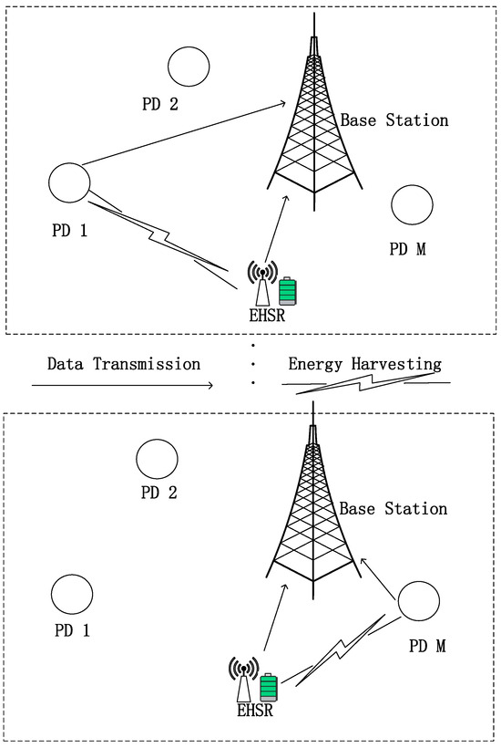
Figure 1. EH symbiotic radio system.

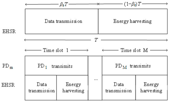
Figure 2. Data transmission mode.

Table 1. Summary of main notations.

Notation	Description
M	Number of primary devices
$S{e}_0$	EH symbiotic radio SD
$t_k$	Any given time slot
$h_k$	Channel gain between BS and $P{D}_k$
$h_{k,0}$	Channel gain between $P{D}_k$ and $S{e}_0$
$h_{0,k}$	Channel gain between $S{e}_0$ and BS
${\beta }_k$	Time allocation factor
$T$	Duration for every time slot
$P_k$	Transmit power of $P{D}_k$
$P_{th}$	Energy harvesting threshold
$\eta$	Energy harvesting efficiency
$E_k$	Residual energy in the battery of $S{e}_0$
$E_{\max }$	Maximum battery capacity of $S{e}_0$
$P_{0,k}$	Transmit power of $S{e}_0$
$P_{\max }$	Maximum transmit power of $S{e}_0$
$\gamma$	Discount rate
$E_k^{\mathrm{sur}}$	Energy surplus
$W_0(\cdot )$	Principal branch of the Lambert W function
$s,s_k$	Current state
${\omega }^{\mu },{\omega }^{{\mu }^{\prime }}$	Parameters of Actor, target Actor network
$n$	Noise
$a(s)=\mu \left(s|{\omega }^{\mu }\right)+n,a_k=\mu \left(s_k|{\omega }^{\mu }\right)+n$	Action
$a^{\prime }(s^{\prime })={\mu }^{\prime }(s^{\prime }|{\omega }^{\mu }),a_{k+1}=\mu (s_{k+1})$	Target action
$F$	Features from the hidden layer of Critic
${\omega }^Q,{\omega }^{Q^{\prime }}$	Parameters of Critic, Critic target network
$Q(\left.s,a\right|{\omega }^Q),Q(\left.s_k,a_k\right|{\omega }^Q)$	Output of the Critic network
$Q^{\prime }(\left.s^{\prime },a^{\prime }\right|{\omega }^{Q^{\prime }}),Q^{\prime }(\left.s_{k+1},a_{k+1}\right|{\omega }^{Q^{\prime }})$	Output of the Critic target network
$r,r_k$	System reward
$s^{\prime },s_{k+1}$	New state
$(s,a,r,s^{\prime }),(s_k,a_k,r_k,s_{k+1})$	Experience tuple
${\epsilon }_k$	Weight
$N$	Batch size
$y_k$	Target value
$\tau$	Update coefficient

In this paper, we employ a piece-wise linear function-based NLPM [41] to calculate the harvested energy during $(1-{\beta }_k)T$.

$$E_{(1-{\beta }_k)T}=\left\{\begin{array}{l}(1-{\beta }_k)T\eta P_k{\left|h_{k,0}\right|}^2, \\ P_{th}(1-{\beta }_k)T , \end{array}\right.\begin{array}{c}\eta P_k{\left|h_{k,0}\right|}^2\le P_{th}\\ \eta P_k{\left|h_{k,0}\right|}^2>P_{th}\end{array}$$

(1)

where $P_k$ is the transmit power of $P{D}_k$, $P_{th}$ denotes the energy harvesting threshold of the EH circuit, and $\eta$ is the energy harvesting efficiency.

Let $E_k$ denote the residual energy in the battery of $S{e}_0$ at the beginning of the time slot $t_k$, after energy harvesting, the energy of $S{e}_0$ in the subsequent time slot $t_{k+1}$ can be formulated as:

$$E_{k+1}=\min \left\{E_{\max },E_{(1-{\beta }_k)T}-{\beta }_{k}T{P}_{0,k}+E_k\right\}$$

(2)

Here, $E_{\max }$ is the maximum battery capacity of $S{e}_0$, ${\beta }_{k}T{P}_{0,k}$ denotes the energy consumed by $S{e}_0$ for data transmission in time slot $t_k$. $P_{0,k}$ is the transmit power of $S{e}_0$, with a maximum value of $E_k$. Based on Formula (2), $S{e}_0$’s transmit power is dynamically constrained by its harvested energy and $E_{\max }$. This energy constraint inherently limits $S{e}_0$’s interference to the co-channel PD, which will guarantee the quality of service (QoS) for PD.

In time slot $t_k$, the achievable data rate of $S{e}_0$ is represented as:

$$R_k={\beta }_k\ln \left({\displaystyle \frac{P_{0,k}{\left|h_{0,k}\right|}^2}{1+P_k{\left|h_k\right|}^2}}+1\right)$$

(3)

The BS first decodes the signal of $S{e}_0$, then removes the signal of $S{e}_0$ to decode the signal of $P{D}_k$ using SIC. Our primary objective is to maximize the long-term throughput of $S{e}_0$. Essentially, this involves a decision-making process for $S{e}_0$ to determine which PD to access at each time slot $t_k$ as well as to optimize its own power and time allocation coefficient to achieve the highest possible throughput over an extended period. The problem can be mathematically formulated as:

$$\begin{array}{ll}\mathrm{P}1:& \underset{P_{0,k},{\beta }_k}{\max }\mathbb{E}\left[{\displaystyle \sum _{k=1}^{\infty }{\gamma }^{k-1}{R}_k}\right]\hspace{1em}\\ s.t.& E_{k+1}=\min \left\{E_{\max },E_{(1-{\beta }_k)T}-{\beta }_{k}T{P}_{0,k}+E_k\right\}(\mathrm{P}1\mathrm{a})\\ & {\beta }_{k}T{P}_{0,k}\le E_k \left(\mathrm{P}1\mathrm{b}\right)\\ & 0\le {\beta }_k\le 1 \left(\mathrm{P}1\mathrm{c}\right)\\ & 0\le P_{0,k}\le P_{\max } \left(\mathrm{P}1\mathrm{d}\right)\end{array}$$

(4)

where $P_{\max }$ denotes the maximum transmit power of $S{e}_0$. $\gamma ,0\le \gamma \le 1$ is the discount rate, which serves as a tradeoff between short-term and long-term rewards. Constraint (P1b) ensures that the energy used for data transmission by $S{e}_0$ does not exceed its remaining energy at time slot $t_k$. The parameter ${\beta }_k$ and $P_{0,k}$ are coupled and have distinct value ranges. This coupling makes it challenging to directly use them as input actions for DRL, as it can result in unstable training.

4. Problem Formulation and Decomposition

4.1. Problem Transformation

Optimization problem P1 is solved via a layered optimization approach. In this section, we design a logic flow diagram to analyze this process (Figure 3).

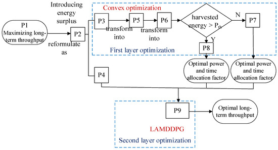
Figure 3. Logic flow diagram for the two-layered optimization process.

We introduce a variable $E_k^{\mathrm{sur}}$ to represent the energy surplus. If $E_k^{\mathrm{sur}}\ge 0$ it indicates that the harvested energy can cover the energy consumed during data transmission. This condition helps extend the operational lifespan of the network, which is a key objective of the system.

$$E_k^{\mathrm{sur}}=E_{(1-{\beta }_k)T}-{\beta }_{k}T{P}_{0,k}$$

(5)

${\beta }_k$ and $P_{0,k}$ can be denoted by $E_k^{\mathrm{sur}}$. Then problem P1 can be transformed into problem P2.

$$\begin{array}{l}\mathrm{P}2:\hspace{1em}\hspace{1em}\underset{{\pi }_{E_k^{\mathrm{sur}}}}{\max }\mathbb{E}\left[{\displaystyle \sum _{k=1}^{\infty }{\gamma }^{k-1}{R}_k}\right]\hspace{1em}\\ s.t.\hspace{1em}{E}_{k+1}=\min \left\{E_{\max },E_k^{\mathrm{sur}}+E_k\right\}\end{array}$$

(6)

In essence, maximizing the long-term throughput of $S{e}_0$ involves optimizing its $E_k^{\mathrm{sur}}$ and ${\beta }_k$. When $E_k^{\mathrm{sur}}=0$, we can obtain:

$$\stackrel{\sim }{R_k}=\sup \left\{\left.R_k\right|E_{(1-{\beta }_k)T}-{\beta }_{k}T{P}_{0,k}=E_k^{\mathrm{sur}},(\mathrm{P}1\mathrm{b}),(\mathrm{P}1\mathrm{c}),(\mathrm{P}1\mathrm{d})\right\}$$

(7)

To maximize the long-term throughput, we can focus on maximizing $R_k$ at each time slot. Specifically, the throughput at each time slot can be optimized by adjusting ${\beta }_k$ and $P_{0,k}$, as follows:

$$\begin{array}{ll}\mathrm{P}3:& \underset{P_{0,k},{\beta }_k}{\max }\hspace{1em}{R}_k\hspace{1em}\\ s.t.& E_{(1-{\beta }_k)T}-{\beta }_{k}T{P}_{0,k}=E_k^{\mathrm{sur}}(\mathrm{P}3\mathrm{a})\\ & (\mathrm{P}1\mathrm{b}),(\mathrm{P}1\mathrm{c}),(\mathrm{P}1\mathrm{d})\end{array}$$

(8)

When $E_k^{\mathrm{sur}}$ is given, we can determine the optimal values of ${\beta }_k$ and $P_{0,k}$ as ${\beta }_k^{\ast }(E_k^{\mathrm{sur}})$ and $(E_k^{\mathrm{sur}})$, respectively. By substituting these optimal values into P2, we can transform P2 in to P4:

$$\begin{array}{l}\mathrm{P}4: \underset{{\pi }_{E_k^{\mathrm{sur}}}}{\max }\mathbb{E}\left[{\displaystyle \sum _{k=1}^{\infty }{\gamma }^{k-1}{R}_k({\beta }_k^{\ast }(E_k^{\mathrm{sur}}),P_{0,k}^{\ast }(E_k^{\mathrm{sur}}))}\right]\hspace{1em}\\ s.t.\hspace{1em} E_{k+1}=\min \left\{E_{\max },E_k^{\mathrm{sur}}+E_k\right\}\end{array}$$

(9)

Thus, problem P1 is decomposed into sub-problems P3 and P4, both of which are closely related to $E_k^{\mathrm{sur}}$. For a given $E_k^{\mathrm{sur}}$, we first solve P3 using convex optimization techniques [42]. Subsequently, P4 can be transformed into a problem solved by the LAMDDPG method.

4.2. Solving Problem P3

Because $E_{(1-{\beta }_k)T}-{\beta }_{k}T{P}_{0,k}=E_k^{\mathrm{sur}}$ is not affine, and constraint (P1b) involves the optimization variable ${\beta }_k$, P3 is a non-convex problem. As indicated in [41], P3 can be reformulated as follows:

$$\begin{array}{l}\mathrm{P}5:\hspace{1em}\hspace{1em}\underset{{\beta }_k}{\max }\hspace{1em}\stackrel{\sim }{f_0}({\beta }_k)\hspace{1em}\\ s.t.\hspace{1em} 0\le {\beta }_k\le 1\end{array}$$

(10)

where $\stackrel{\sim }{f_0}({\beta }_k)=\sup \left\{\left.R_k\right|E_{(1-{\beta }_k)T}-{\beta }_{k}T{P}_{0,k}-E_k^{\mathrm{sur}}=0,(\mathrm{P}1\mathrm{b}),(\mathrm{P}1\mathrm{d})\right\}$.

Following the formula $E_{(1-{\beta }_k)T}-{\beta }_{k}T{P}_{0,k}-E_k^{\mathrm{sur}}=0$, we can derive an expression for $P_{0,k}$ as following:

$$P_{0,k}=\left\{\begin{array}{l}{\displaystyle \frac{(1-{\beta }_k)T\eta P_k{\left|h_{k,0}\right|}^2-E_k^{\mathrm{sur}}}{{\beta }_{k}T}}, \\ {\displaystyle \frac{P_{th}(1-{\beta }_k)T-E_k^{\mathrm{sur}}}{{\beta }_{k}T}} , \end{array}\right.\begin{array}{c}\eta P_k{\left|h_{k,0}\right|}^2\le P_{th}\\ \eta P_k{\left|h_{k,0}\right|}^2>P_{th}\end{array}$$

(11)

According to constraint (P1b), we can obtain:

$$P_{0,k}\le {\displaystyle \frac{E_k}{{\beta }_{k}T}}$$

(12)

Thus finding $\stackrel{\sim }{f_0}({\beta }_k)$ is equivalent to solving the optimization problem:

$$\begin{array}{ll}\mathrm{P}6:& \underset{P_{0,k}}{\max }\hspace{1em}{R}_k\hspace{1em}\\ s.t.& P_{0,k}={\displaystyle \frac{E_{(1-{\beta }_k)T}-E_k^{\mathrm{sur}}}{{\beta }_{k}T}} \left(\mathrm{P}6\mathrm{a}\right) \\ & P_{0,k}\le {\displaystyle \frac{E_k}{{\beta }_{k}T}} \left(\mathrm{P}6\mathrm{b}\right) \\ & 0\le P_{0,k}\le P_{\max } \left(\mathrm{P}6\mathrm{c}\right) \end{array}$$

(13)

Problem P6 is a function of $P_{0,k}$, where ${\beta }_k$ is fixed. Given the constraints (P6a), $\stackrel{\sim }{f_0^{\ast }}({\beta }_k)$ can be expressed as:

$$\stackrel{\sim }{f_0^{\ast }}({\beta }_k)={\beta }_k\ln \left({\displaystyle \frac{\frac{E_{(1-{\beta }_k)T}-E_k^{\mathrm{sur}}}{{\beta }_{k}T}{\left|h_{0,k}\right|}^2}{1+P_k{\left|h_k\right|}^2}}+1\right)$$

(14)

The constraints (P6b) and (P6c) can be satisfied by specifying the domain of $\stackrel{\sim }{f_0^{\ast }}({\beta }_k)$ as:

$$\mathcal{D}=\left\{\left.{\beta }_k\right|0\le {\displaystyle \frac{E_{(1-{\beta }_k)T}-E_k^{\mathrm{sur}}}{{\beta }_{k}T}}\le \min \left\{P_{\max },{\displaystyle \frac{E_k}{{\beta }_{k}T}}\right\}\right\}$$

(15)

By Formulas (8) and (9), when $\eta P_k{\left|h_{k,0}\right|}^2\le P_{th}$, P6 can be denoted as:

$$\begin{array}{ll}\mathrm{P}7:& \underset{{\beta }_k}{\max }{\beta }_k\ln \left({\displaystyle \frac{\frac{E_{(1-{\beta }_k)T}-E_k^{\mathrm{sur}}}{{\beta }_{k}T}{\left|h_{0,k}\right|}^2}{1+P_k{\left|h_k\right|}^2}}+1\right)\hspace{1em}\\ s.t.& {\beta }_k\le 1-{\displaystyle \frac{E_k^{\mathrm{sur}}}{T\eta P_k{\left|h_{k,0}\right|}^2}} \hspace{0.17em}\left(\mathrm{P}7\mathrm{a}\right) \\ & {\beta }_k\ge 1-{\displaystyle \frac{E_k+E_k^{\mathrm{sur}}}{T\eta P_k{\left|h_{k,0}\right|}^2 }} \left(\mathrm{P}7\mathrm{b}\right) \\ & {\beta }_k\ge {\displaystyle \frac{T\eta P_k{\left|h_{k,0}\right|}^2-E_k^{\mathrm{sur}}}{T\eta P_k{\left|h_{k,0}\right|}^2+T{P}_{\max } }} \left(\mathrm{P}7\mathrm{c}\right)\\ & 0\le {\beta }_k\le 1 \hspace{0.17em}\left(\mathrm{P}7\mathrm{d}\right) \end{array}$$

(16)

When $\eta P_k{\left|h_{k,0}\right|}^2>P_{th}$, P6 can be denoted as:

$$\begin{array}{ll}\mathrm{P}8:& \underset{{\beta }_k}{\max }{\beta }_k\ln \left({\displaystyle \frac{\frac{E_{(1-{\beta }_k)T}-E_k^{\mathrm{sur}}}{{\beta }_{k}T}{\left|h_{0,k}\right|}^2}{1+P_k{\left|h_k\right|}^2}}+1\right)\hspace{1em}\\ s.t.& {\beta }_k\le 1-{\displaystyle \frac{E_k^{\mathrm{sur}}}{P_{th}T }} \hspace{0.17em}\left(\mathrm{P}8\mathrm{a}\right) \\ & {\beta }_k\ge 1-{\displaystyle \frac{E_k+E_k^{\mathrm{sur}}}{P_{th}T }} \hspace{0.17em}\left(\mathrm{P}8\mathrm{b}\right)\\ & {\beta }_k\ge {\displaystyle \frac{P_{th}T-E_k^{\mathrm{sur}}}{P_{th}T+P_{\max }T }} \left(\mathrm{P}8\mathrm{c}\right)\\ & 0\le {\beta }_k\le 1 \left(\mathrm{P}8\mathrm{d}\right) \\ \end{array}$$

(17)

Both P7 and P8 involve three lower bounds and two upper bounds related to ${\beta }_k$. Moreover, the objective functions in P7 and P8 impose constraints on the selection of ${\beta }_k$. Therefore, it is crucial to demonstrate the feasibility of the optimization problems P7 and P8. The proof of the feasibility of problems P7 and P8 is provided in Appendix A. In addition, we prove that P7 and P8 are concave functions of ${\beta }_k,{\beta }_k\ge 0,$ in Appendix B.

The substantial number of inequality constraints in problems P7 and P8 complicated the process of obtaining an optimal solution for ${\beta }_k^{\ast }\left(E_k^{\mathrm{sur}}\right)$. Moreover, the first-order derivative of the objective function takes the form of the Lambert W function with two branches [27]. Following the steps outlined in [27], if $E_k^{\mathrm{sur}}$ satisfies:

$$E_k^{\mathrm{sur}}\ne \left\{\begin{array}{l}T\eta P_k{\left|h_{k,0}\right|}^2, \\ P_{th}T , \end{array}\right.\begin{array}{c}\eta P_k{\left|h_{k,0}\right|}^2\le P_{th}\\ \eta P_k{\left|h_{k,0}\right|}^2>P_{th}\end{array}$$

(18)

otherwise ${\beta }_k^{\ast }\left(E_k^{\mathrm{sur}}\right)=0$, we can achieve a closed form for ${\beta }_k^{\ast }\left(E_k^{\mathrm{sur}}\right)$, as follows:

$${\beta }_k^{\ast }(E_k^{\mathrm{sur}})=\left\{\begin{array}{l}\min \left\{1,\max \left\{{\displaystyle \frac{{\lambda }_1-{\lambda }_2}{e^{W_0(e^{-1}({\lambda }_1-1))+1}-1+{\lambda }_1}},{\zeta }_0\right\}\right\}, \\ \min \left\{1,\max \left\{{\displaystyle \frac{{\lambda }_3-{\lambda }_2}{e^{W_0(e^{-1}({\lambda }_3-1))+1}-1+{\lambda }_3}},{\zeta }_1\right\}\right\} , \end{array}\right.\begin{array}{c}\eta P_k{\left|h_{k,0}\right|}^2\le P_{th}\\ \eta P_k{\left|h_{k,0}\right|}^2>P_{th}\end{array}$$

(19)

where $W_0(\cdot )$ denotes the principal branch of the Lambert W function [43]. ${\lambda }_1={\displaystyle \frac{\eta P_k{\left|h_{k,0}\right|}^2}{(1+P_k{\left|h_k\right|}^2)}}{\left|h_{0,k}\right|}^2$, ${\lambda }_2={\displaystyle \frac{E_k^{\mathrm{sur}}{\left|h_{0,k}\right|}^2}{T(1+P_k{\left|h_k\right|}^2)}}$, ${\lambda }_3={\displaystyle \frac{P_{th}}{(1+P_k{\left|h_k\right|}^2)}}{\left|h_{0,k}\right|}^2$, ${\zeta }_0=\max \left\{1-{\displaystyle \frac{E_k+E_k^{\mathrm{sur}}}{T\eta P_k{\left|h_{k,0}\right|}^2 }},{\displaystyle \frac{T\eta P_k{\left|h_{k,0}\right|}^2-E_k^{\mathrm{sur}}}{T\eta P_k{\left|h_{k,0}\right|}^2+T{P}_{\max } }}\right\}$, ${\zeta }_1=\max \left\{1-{\displaystyle \frac{E_k+E_k^{\mathrm{sur}}}{P_{th}T }},{\displaystyle \frac{P_{th}T-E_k^{\mathrm{sur}}}{P_{th}T+P_{\max }T }}\right\}$.

Based on ${\beta }_k^{\ast }\left(E_k^{\mathrm{sur}}\right)$, the optimal power allocation coefficient is achieved by:

$$P_{0,k}^{\ast }(E_k^{\mathrm{sur}})=\left\{\begin{array}{l}{\displaystyle \frac{(1-{\beta }_k^{\ast })\eta P_k{\left|h_{k,0}\right|}^2}{{\beta }_k^{\ast }}}-{\displaystyle \frac{E_k^{\mathrm{sur}}}{{\beta }_k^{\ast }T}}, \\ {\displaystyle \frac{(1-{\beta }_k^{\ast })P_{th}}{{\beta }_k^{\ast }}}-{\displaystyle \frac{E_k^{\mathrm{sur}}}{{\beta }_k^{\ast }T}} , \end{array}\right.\begin{array}{c}\eta P_k{\left|h_{k,0}\right|}^2\le P_{th}\\ \eta P_k{\left|h_{k,0}\right|}^2>P_{th}\end{array}$$

(20)

If $E_k^{\mathrm{sur}}$ satisfies:

$$E_k^{\mathrm{sur}}=\left\{\begin{array}{l}T\eta P_k{\left|h_{k,0}\right|}^2, \\ P_{th}T , \end{array}\right.\begin{array}{c}\eta P_k{\left|h_{k,0}\right|}^2\le P_{th}\\ \eta P_k{\left|h_{k,0}\right|}^2>P_{th}\end{array}$$

(21)

$S{e}_0$ harvests energy at the whole time slot, there is no data transmission, and there is no need to specify the value for $P_{0,k}^{\ast }(E_k^{\mathrm{sur}})$.

4.3. Solving Problem P4

With ${\beta }_k^{\ast }(E_k^{\mathrm{sur}})$ and $P_{0,k}^{\ast }(E_k^{\mathrm{sur}})$ obtained, the long-term throughput maximizing problem is reformulated as:

$$\begin{array}{l}\mathrm{P}9:\hspace{1em}\hspace{1em}\underset{{\pi }_{E_k^{\mathrm{sur}}}}{\max }\mathbb{E}\left[{\displaystyle \sum _{k=1}^{\infty }{\gamma }^{k-1}{\beta }_k^{\ast }(E_k^{\mathrm{sur}})\ln \left(\frac{P_{0,k}^{\ast }(E_k^{\mathrm{sur}}){\left|h_{0,k}\right|}^2}{1+P_k{\left|h_k\right|}^2}+1\right)}\right]\hspace{1em}\\ s.t.\hspace{1em} E_{k+1}=\min \left\{E_{\max },E_k^{\mathrm{sur}}+E_k\right\} \left(\mathrm{P}9\mathrm{a}\right) \end{array}$$

(22)

This problem is a function of $E_k^{\mathrm{sur}}$, which can be optimized through the LAMDDPG method.

5. Proposed LAMDDPG Algorithm

5.1. Framework of LAMDDPG Algorithm

The optimal long-term throughput decision for P9 is served as a Markov Decision Process (MDP) and solved by the LAMDDPG framework. Here, $S{e}_0$ acts as an agent. The LAMDDPG framework is employed to identify a sequence of optimal decisions that maximizes the long-term expected cumulative discounted reward.

As shown in Figure 4, the LAMDDPG framework contains an Actor network ${\omega }^{\mu }$ and Actor target network ${\omega }^{{\mu }^{\prime }}$, Critic network ${\omega }^Q$ and Critic target network ${\omega }^{Q^{\prime }}$, an experience replay memory. The LSTM layers are integrated after the input layer for Actor network and the Actor target network. The attention layers are adopted after hidden layers for the Critic network and Critic target network.

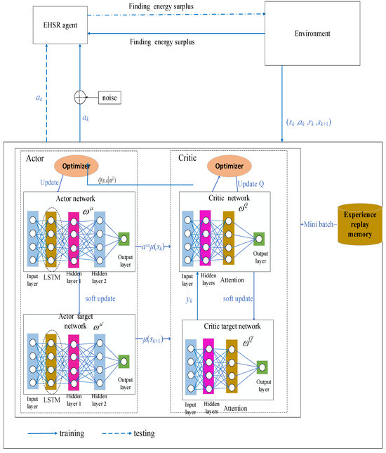
Figure 4. The framework of LAMDDPG. Black solid lines denote the agent, environment, network components, black dashed lines illustrate the network structure of the proposed LAMDDPG algorithm, blue solid lines depict the training phase, blue dashed lines illustrate the execution phase of the algorithm.

The current state $s$ from the environment are input to the Actor and Actor target network, considering the temporal correlation of residual energy and channel state information in the current scenario, LSTM layers are introduced to capture dynamic dependencies. The LSTM layers learn from past observations to adjust the weights and bias to predict the real-time state. The output data is input into the hidden layer of the Actor network ${\omega }^{\mu }$ and Actor target network ${\omega }^{{\mu }^{\prime }}$, respectively. The action $a(s)=\mu \left(s|{\omega }^{\mu }\right)$ and target action ${\mu }^{\prime }\left(s|{\omega }^{{\mu }^{\prime }}\right)$ are output. To enhance the exploration capability of the Actor network, noise is introduced in the output of the Actor network. Thus, the action to be chosen is $a(s)=\mu \left(s|{\omega }^{\mu }\right)+n$, where $n$ represents the noise following a Gaussian distribution.

Moreover, attention mechanisms are integrated into the Critic network and Critic target network. $F$ from the hidden layer are input into the attention module. Through squeezing and excitation, features of different channels are assigned distinct channel weights. By multiplying $F$ with the channel weights, $F$ can be adaptively enhanced, the Critic network can dynamically focus on more important features most relevant to the current agent’s decision-making, thereby enhancing the accuracy of decision-making. The Critic network ${\omega }^Q$ outputs the state-action value function $Q(\left.s,a\right|{\omega }^Q)$ under the current state and action by the Actor network. The Critic target network ${\omega }^{Q^{\prime }}$ outputs $Q^{\prime }(\left.s,a\right|{\omega }^{Q^{\prime }})$. Optimal actions generated by these networks are applied to the environment to obtain a reward $r$, and then the environment transitions to a new state $s^{\prime }$. The experience $(s,a,r,s^{\prime })$ is then stored in the replay memory.

The state space, action space, and reward function are defined as follows

State space: In this CR-NOMA-enabled EHSR network, the state space is defined as the channel state information associated with the PD and $S{e}_0$, the residual energy of $S{e}_0$. The system state at time slot $t_k$ can be denoted as:

$$s_k=(h_{0,k}, h_k, h_{k,0}, E_k)$$

(23)

Action space: The agent selects transmitting data or energy harvesting according to the current system state

$$a_k=E_k^{\mathrm{sur}}$$

(24)

Considering the extreme situation that $S{e}_0$ only transmits data for the whole time slot $t_k$, the lower bound is:

$$E_k^{\mathrm{sur}}\ge -\min \left\{E_k,T{P}_{\max }\right\}$$

(25)

On the other hand, if $S{e}_0$ only harvests energy for the whole time slot $t_k$, the upper bound is:

$$E_k^{\mathrm{sur}}\le \left\{\begin{array}{l}\min \left\{E_{\max }-E_k,T\eta P_k{\left|h_{k,0}\right|}^2\right\}, \\ \min \left\{E_{\max }-E_k,P_{th}T \right\} , \end{array}\right.\begin{array}{c}\eta P_k{\left|h_{k,0}\right|}^2\le P_{th}\\ \eta P_k{\left|h_{k,0}\right|}^2>P_{th}\end{array}$$

(26)

Thus, the value for action is very large, which brings instability to the network. The value of $E_k^{\mathrm{sur}}$ can be normalized as

$$E_k^{\mathrm{sur}}=-(1-{\epsilon }_k)\min \left\{E_k,T{P}_{\max }\right\}+{\epsilon }_k\left\{\begin{array}{l}\min \left\{E_{\max }-E_k,T\eta P_k{\left|h_{k,0}\right|}^2\right\}, \\ \min \left\{E_{\max }-E_k,P_{th}T \right\} , \end{array}\right.\begin{array}{c}\eta P_k{\left|h_{k,0}\right|}^2\le P_{th}\\ \eta P_k{\left|h_{k,0}\right|}^2>P_{th}\end{array}$$

(27)

where ${\epsilon }_k\in \left[0,1\right]$, hence, the suitable action parameter can be constrained to improve the stability of the networks.

Reward function: When the agent selects an action at any time slot $t_k$, it will receive a corresponding reward, set as

$$r_k=R_k$$

(28)

where $R_k$ is the achievable data rate at $t_k$.

The LAMDDPG algorithm employs centralized training with distributed execution. During the training phase, a batch of experience $\mathcal{B}=\left\{(s_k,a_k,r_k,s_{k+1}),k=1,\dots ,N\right\}$ is selected from the replay memory for training, $N$ is the batch size.

The predicted action $a_{k+1}=\mu (s_{k+1})$ is fed into the Critic target network. Based on these inputs, the Critic target network computes the target value $y_k$. The target value for the state function is calculated by:

$$y_k=r_k+\gamma Q^{\prime }(s_{k+1},a_{k+1}|{\omega }^{Q^{\prime }})$$

(29)

$s_k$ and $a_k=\mu (s_k)$ are fed into the Critic network. Based on these inputs, the Critic network calculates the corresponding Q value, denoted as $Q(\left.s_k,a_k\right|{\omega }^Q)$. The parameters of the Critic network are updated using gradient descent. The loss function for the Critic network is defined as the difference between the target value $y_k$ and the predicted $Q(\left.s_k,a_k\right|{\omega }^Q)$, which is essentially the error term of the Bellman equation. Therefore, the parameters of the Critic network can be updated according to the following formula:

$$L\mathrm{oss}({\omega }^Q)=E{[(Q\left(s_k,a_k|{\omega }^Q\right)-y_k))}^2]$$

(30)

When updating the parameters of the Actor network, gradient ascent is employed. The parameters can be updated according to the following formula:

$$\begin{array}{l}{\nabla }_{{\omega }^{\mu }}J\approx E[{\nabla }_{{\omega }^{\mu }}Q\left(s,a|{\omega }^Q\right){|}_{s=s_k,a=\mu (s_k|{\omega }^{\mu })}]\\ =E[{\nabla }_{a}Q\left(s,a|{\omega }^Q\right){|}_{s=s_k,a=\mu (s_k)}{\nabla }_{{\omega }^{\mu }}\mu \left(s|{\omega }^{\mu }\right)|s=s_k]\end{array}$$

(31)

The parameters of both target networks are updated using a soft update method, described as follows:

$${\omega }^{{\mu }^{\prime }}\leftarrow \tau {\omega }^{\mu }+(1-\tau ){\omega }^{{\mu }^{\prime }}$$

(32)

$${\omega }^{Q^{\prime }}\leftarrow \tau {\omega }^Q+(1-\tau ){\omega }^{Q^{\prime }}$$

(33)

where $\tau$ is the update coefficient.

5.2. Neural Network Architectures and Training Parameters

In this subsection, we present the neural network architecture of the proposed LAMDDPG algorithm. In the LAMDDPG algorithm, both the Actor network and Actor target network contain an input layer, an LSTM layer, two hidden layers, and an output layer. Both the Critic network and Critic target network consist of an input layer, two hidden layers, an attention module (based on the Squeeze-and-Excitation module), and an output layer. Both the Actor and Critic networks adopt the Adam optimizer.

The input layer of the Actor (target) network takes the state $s$ as input, performing input reshaping to adapt to the input format required by the LSTM layer. The LSTM layer contains 64 units and outputs a vector with a dimension of (32, 64), which is fed into the first hidden layer. After ReLU activation, the first hidden layer outputs a vector of (32, 64), which is then passed to the second hidden layer. Following tanh activation, the second hidden layer outputs a (32, 64) vector that is fed into the output layer. After tanh activation, the output action is scaled to the range between the maximum and minimum magnitudes of the action (target action).

The Critic (target) network takes the state $s$ ($s^{\prime }$) and action $a$ ($a^{\prime }$) as inputs. These inputs undergo feature fusion in the first hidden layer, and after ReLU activation, a vector with a dimension of (32, 64) is output. This vector is fed into the second hidden layer, which outputs a feature vector of dimension (32, 64) following ReLU activation. Subsequently, the vector enters the attention module: first, average pooling is performed on the feature dimension to complete the squeezing operation; then, it passes through two fully connected layers, activated by ReLU and Sigmoid, respectively, to generate channel-wise attention weights. The vectors are then multiplied by the attention weights to obtain an output vector of (32, 64). Finally, the action value function $Q$ ($Q^{\prime }$) is output after passing through the output layer.

The LAMDDPG algorithm is presented in the LAMDDPG algorithm (Algorithm 1).

Algorithm 1 LAMDDPG algorithm
Input: Environment, settings of $S{e}_0$ and PDs Output: parameters ${\omega }^{\mu }, {\omega }^{{\mu }^{\prime }}, {\omega }^Q, {\omega }^{Q^{\prime }}$ Initialize system parameters, initialize Actor network, and Critic network
Initialize target network weights parameters
Initialize experience replay memory
1	For episode = 1 to nep, do:
2	Initialization of noise n, initialization of large-scale fading, and small-scale random fading
3	Obtain the initial state s1
4	For k = 1 to T, do:
5	Select $a_k=\mu \left(s_k|{\omega }^{\mu }\right)+n$
6	Execute action ak, receive reward rk, and environment state sk+1, and store the array $\left(s_k,a_k,r_k,s_{k+1}\right)$ in the experience replay memory
7	Randomly sample a batch of experience $\mathcal{B}=\left\{(s_k,a_k,r_k,s_{k+1}),k=1,\dots ,N\right\}$ from the replay memory
8	Set $y_k=r_k+\gamma Q^{\prime }(s_{k+1},a_{k+1}|{\omega }^{Q^{\prime }})$
9	Minimize the loss function to update the Critic Q network
	$L\mathrm{oss}({\omega }^Q)=E{[(Q\left(s_k,a_k|{\omega }^Q\right)-y_k))}^2]$
10	Sample strategy gradient update Actor policy network
	${\nabla }_{{\omega }^{\mu }}J\left({\omega }^{\mu }\right)=E[{\nabla }_{a}Q\left(s,a|{\omega }^Q\right){|}_{s=s_k,a=\mu (s_k)}{\nabla }_{{\omega }^{\mu }}\mu \left(s|{\omega }^{\mu }\right)|s=s_k]$
11	Update target network
	${\omega }^{{\mu }^{\prime }}\leftarrow \tau {\omega }^{\mu }+(1-\tau ){\omega }^{{\mu }^{\prime }},{\omega }^{Q^{\prime }}\leftarrow \tau {\omega }^Q+(1-\tau ){\omega }^{Q^{\prime }}$
12	End for
13	End for

6. Simulation Results

In this section, we prove the effectiveness of the proposed algorithm. The path loss model from [13] is adopted, with the following parameter settings in Table 2 [27].

Table 2. Parameter settings.

Parameter Settings
Learning rate of the Actor network	0.002
Learning rate of the Critic network	0.004
discount rate $\gamma$	0.9
Network update parameters $\tau$	0.01
Batch size of experience replay pool	32
transmission power of $P_k$	30 dBm
initial energy $E_{\max }$	0.1 J
The duration of each time slot T	1 s
The maximum transmission power of $P_{\max }$	0.1 W
Energy harvesting efficiency $\eta$	0.7
Noise power spectral density	−170 dBm/Hz
Bandwidth of noise	1 MHz
Noise carrier frequency	914 MHz
Path Loss Exponent	3
Number of hidden layer nodes	64

BS is located at the origin of the x-y plane. $S{e}_0$ is deployed at (1 m, 1 m). To compare the performance of the LAMDDPG algorithm, the following baseline algorithms are introduced:

(1)

DDPG algorithm: using the baseline algorithm proposed in [27].

(2)

Greedy algorithm: $S{e}_0$ consumes all battery energy during the data transmission and then begins energy harvesting [27].

(3)

Random algorithm: $S{e}_0$ transmit data using $P_{\max }$ as the transmit power, ${\beta }_k$ is randomly generated between 0 and $\min \left\{1,{\displaystyle \frac{E_k}{T{P}_{\max }}}\right\}$.

(4)

LMDDPG algorithm: To demonstrate the effect of LSTM and attention mechanisms, we design the LMDDPG algorithm by incorporating LSTM layers into the Actor networks of DDPG.

The channels remain unchanged in each experiment, consisting of multiple episodes. Independent and identically distributed (i.i.d.) complex Gaussian random variables with a mean of zero and a unit variance are employed to simulate small-scale fading.

6.1. Rewards Analysis Under Different Algorithms

We first examine the data rate performance of different algorithms when M = 2, corresponding to two PDs positioned at (0 m, 1 m) and (0 m, 1000 m). As illustrated in Figure 5, after independent and repeated experiments, the data rates achieved by the DDPG, LMDDPG, and LAMDDPG algorithms significantly surpass those of the Greedy and Random algorithms. This superiority stems from the fact that $S{e}_0$ can choose optimal actions under the guidance of DRL algorithms effectively. The incorporation of LSTM layers in the Actor networks enables LMDDPG to converge faster than DDPG. Furthermore, the integration of attention mechanisms into the Critic networks allows the LAMDDPG algorithm to converge at the 50th episode while the data rate increases by 19% over LMDDPG. The combination of LSTM and attention mechanisms improves the data rate by 25% over DDPG.

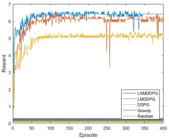
Figure 5. Rewards under different algorithms when M = 2.

Next, we investigate the data rate performance of various algorithms under different numbers of PDs. Figure 6a,b shows scenarios with 5 PDs and 10 PDs in the network, respectively. These PDs are positioned between (0 m, 1 m) and (0 m, 1000 m). In these complex and dynamic environments with more PDs, both the Random and Greedy algorithms achieve very low data rates. As depicted in Figure 6a,b, after independent and repeated experiments, the data rates achieved by DDPG, LMDDPG, and LAMDDPG algorithms obviously surpass those of the Greedy and Random algorithms. When the number of PDs is 5, the maximum data rate achieved by LAMDDPG is nearly 8 bps. As the number of PDs increases to 10, the maximum data rate achieved by LAMDDPG rises to nearly 10 bps. The LAMDDPG algorithm converges faster than LMDDPG and DDPG in Figure 6a,b. However, compared with Figure 6a, LAMDDPG converges more slowly in Figure 6b, due to the increase in the number of PDs participating in NOMA transmission leads to an increase in the state space of the DRL algorithms, which consequently results in a slower convergence rate. On the other hand, the data rates in Figure 6a,b are higher than those in Figure 5. This is because with more PDs involved, there is relatively more time available for $S{e}_0$ to transmit data.

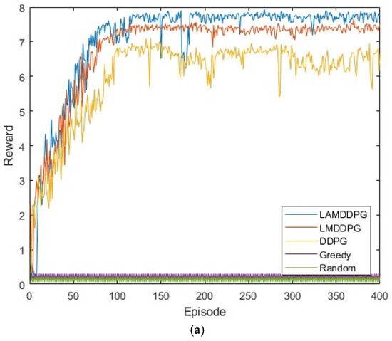
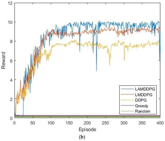
Figure 6. (a) Rewards under different algorithms when M = 5. (b) Rewards under different algorithms when M = 10.

6.2. Rewards Analysis Under Different EH Model

We then investigate the performance of different algorithms under various EH models when M = 2. In Figure 7, real indicates the EH model based on NLPM, which is more practical in real environments, while ideal indicates the EH model based on the linear model, commonly used in theoretical analyses. Two PDs are positioned at (0 m, 1 m) and (0 m, 1000 m), respectively. As depicted in Figure 7, after independent and repeated experiments, the upper bound of data rate is 5 bps achieved by the DDPG algorithm with the linear EH model. Under the NLPM, the data rate of DDPG reaches nearly 4.6 bps, which is smaller than that of LAMDDPG with NLPM, achieving nearly 5 bps. The LAMDDPG algorithm converges approximately at 50 episodes to achieve the maximal data rate. This superiority stems from the ability of the LAMDDPG algorithm to help $S{e}_0$ to choose optimal actions through the combination of LSTM and attention mechanisms.

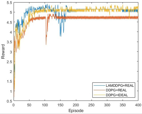
Figure 7. Rewards under different EH models when M = 2.

We further investigate the performance of different algorithms under various EH models with different numbers of PDs. Here, real indicates the EH model based on the NLPM, while ideal denotes the EH model based on the linear model. Figure 8a and Figure 8b show scenarios with five and ten PDs in the network, respectively. These PDs are positioned between (0 m, 1 m) and (0 m, 1000 m). As depicted in Figure 8a,b, after independent and repeated experiments, the upper bound of the data rates is 7 bps and 8 bps, respectively, achieved by the DDPG algorithm with the linear EH model. The maximum data rate increases with the number of PDs participating in NOMA transmission, due to more PDs providing more opportunities for $S{e}_0$ transmitting data. Under the NLPM, the data rates of DDPG in Figure 8a,b reach nearly 5.8 bps and 6 bps, respectively, which are lower than those of LAMDDPG with NLPMs. The data rates of LAMDDPG with NLPM achieve the maximum data rates in both Figure 8a,b. Compared with Figure 8a, when there are ten PDs, the rapid increase in states caused by the growing number of PDs participating in NOMA transmission results in a slower convergence speed, and increased fluctuation under NPLM in Figure 8b.

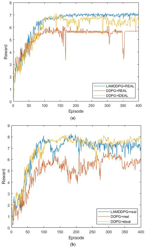
Figure 8. (a) Rewards under different EH models when M = 5. (b) Rewards under the different EH models when M = 10.

6.3. Mechanism Analysis of Performance Improvement

Through ablation experiments (Figure 5, Figure 6, Figure 7 and Figure 8), we compare the LMDDPG algorithm with an added LSTM layer, the LAMDDPG algorithm (integrating LSTM and attention mechanisms), and DDPG, Greedy, and Random algorithms. The simulation results demonstrate that LAMDDPG achieves faster convergence and higher cumulative rewards across scenarios with varying numbers of PDs and different energy-harvesting models.

In our scenario, inherent dependencies exist between CSI and the remaining energy of EHSR. The introduced LSTM layer leverages its hidden state to encode historical data, enabling the agent to capture implicit states that are critical for decision-making. Thus, LMDDPG outperforms DDPG, greedy, and random algorithms in reward accumulation.

By integrating the attention module, the extracted features from hidden layers of the Critic (target) network are squeezed and activated by the Sigmoid function, which mitigates the overestimation bias of Q-values. Meanwhile, by squeeze-excitation-scaling steps, the attention module adaptively assigns weights to the extracted features, which emphasizes those that contribute more to Q-value estimation while suppressing redundant ones. This enhances the accuracy of Q-value predictions, reducing the agent’s ineffective exploration and thus accelerating algorithm convergence while boosting cumulative rewards.

6.4. Rewards Analysis Under Different Numbers of PDs

Furthermore, we deploy more PDs to investigate the maximum data rate under different PDs according to different EH models. As depicted in Figure 9, the average data rate initially increases with the increase in PDs, then decreases with the increase in PDs under different algorithms. This is because when the number of PDs exceeds two, the system allocates more time slots, thereby enhancing the data rate. However, when the number of PDs surpasses 10, the system experiences a sharp decline due to the strong inter-device interference caused by the increased number of PDs. As seen from Figure 10, when PD = 10, $S{e}_0$ is more inclined to select actions for data transmission than to conserve energy compared with the scenario where the number is 15. In other words, the action corresponds to the surplus energy, and the probability of the surplus energy being small is relatively high. As seen from Figure 11, when the number of PD is 15, the probability of the surplus energy being large is relatively high, indicating that $S{e}_0$ tends to prioritize energy harvesting over data transmission to manage the increased interference, which further contributes to the decline in data rate. Regarding the algorithms, LAMDDPG demonstrates a superior data rate compared to DDPG under NLPM, indicating that the LSTM and attention mechanism are more effective in managing the complex environments. Moreover, the system can achieve ideal values under the linear EH model, due to the linear EH model providing a more favorable environment. The optimal data rate can be achieved when the number of PDs is ten, highlighting the importance of balancing the number of PDs to maintain efficient network performance.

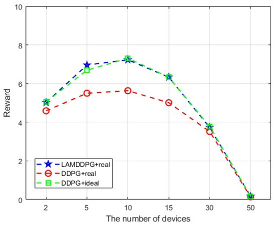
Figure 9. Rewards under different numbers of PDs.

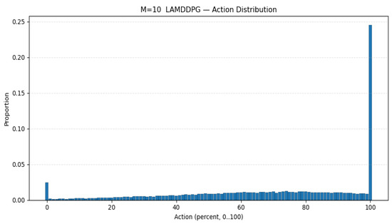
Figure 10. Action selection when PD = 10.

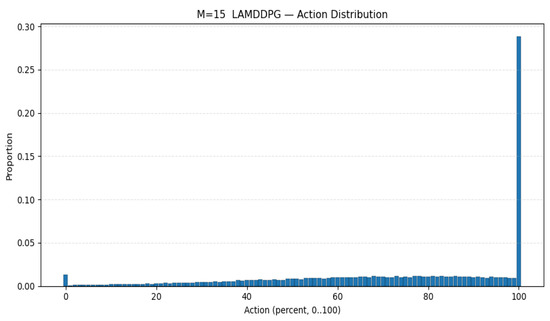
Figure 11. Action selection when PD = 15.

7. Conclusions

In this paper, we consider the long-term throughput maximization problem for an EHSR IoT device in a CR-NOMA-enabled IoT network that comprises multiple primary IoT devices, a base station, and an EHSR IoT device. To be closer to practical applications, we adopt a piece-wise linear function-based NLPM. We addressed this optimization problem by integrating convex optimization with the LAMDDPG algorithm. Experimental results demonstrate that the LSTM layer in the Actor network can predict channel state information from historical data, effectively solving the agent’s partial observability problem. Meanwhile, the channel attention SE block in the Critic network mitigates Q-value overestimation in DRL algorithms through squeeze-excitation-scale operations. The synergy of these two mechanisms accelerates exploration, improves reward acquisition, and speeds up convergence. Moreover, we find the optimal number of PDs to maintain efficient network performance under NLPM, which is highly significant for guiding practical EHSR applications. However, we consider the ideal SIC condition in such an EH-CR-NOMA symbiotic system. In future work, we will extend our research to non-ideal SIC scenarios and further explore improving other types of DRL algorithms (e.g., PPO, TD3) to address the throughput maximization problem in EH-CR-NOMA symbiotic networks with a nonlinear energy harvesting model.

References

- Donta, P.K.; Srirama, S.N.; Amgoth, T.; Annavarapu, C.S.R. Survey on recent advances in IoT application layer protocols and machine learning scope for research directions. Digit. Commun. Netw. 2022, 8, 727–744. [Google Scholar] [CrossRef]
- Andrews, J.G.; Buzzi, S.; Choi, W.; Hanly, S.V.; Lozano, A.; Soong, A.K.; Zhang, J.C. What will 5G be? IEEE J. Sel. Areas Commun. 2014, 32, 1065–1082. [Google Scholar] [CrossRef]
- Makki, B.; Chitti, K.; Behravan, A.; Alouini, M.-S. A survey of NOMA: Current status and open research challenges. IEEE Open J. Commun. Soc. 2020, 1, 179–189. [Google Scholar] [CrossRef]
- Lei, H.; She, X.; Park, K.-H.; Ansari, I.S.; Shi, Z.; Jiang, J.; Alouini, M.-S. On secure CDRT with NOMA and physical-layer network coding. IEEE Trans. Commun. 2023, 71, 381–396. [Google Scholar] [CrossRef]
- Kilzi, A.; Farah, J.; Nour, C.A.; Douillard, C. Mutual successive interference cancellation strategies in NOMA for enhancing the spectral efficiency of CoMP systems. IEEE Trans. Commun. 2020, 68, 1213–1226. [Google Scholar] [CrossRef]
- Li, X.; Zheng, Y.; Khan, W.U.; Zeng, M.; Li, D.; Ragesh, G.K.; Li, L. Physical layer security of cognitive ambient backscatter communications for green Internet-of-Things. IEEE Trans. Green Commun. Netw. 2021, 5, 1066–1076. [Google Scholar] [CrossRef]
- Chen, B.; Chen, Y.; Chen, Y.; Cao, Y.; Zhao, N.; Ding, Z. A novel spectrum sharing scheme assisted by secondary NOMA relay. IEEE Wirel. Commun. Lett. 2018, 7, 732–735. [Google Scholar] [CrossRef]
- Do, D.-T.; Le, A.-T.; Lee, B.M. NOMA in Cooperative Underlay Cognitive Radio Networks Under Imperfect SIC. IEEE Access 2020, 8, 86180–86195. [Google Scholar] [CrossRef]
- Ali, Z.; Khan, W.U.; Sidhu, G.A.S.; K, N.; Li, X.; Kwak, K.S.; Bilal, M. Fair power allocation in cooperative cognitive systems under NOMA transmission for future IoT networks. Alex. Eng. J. 2022, 61, 575–583. [Google Scholar] [CrossRef]
- Jiang, Q.; Zhang, C.; Zheng, W.; Wen, X. Research on Delay DRL in Energy-Constrained CR-NOMA Networks based on Multi-Threads Markov Reward Process. In Proceedings of the 2022 IEEE 8th International Conference on Computer and Communications (ICCC), Nanjing, China, 29 March–1 April 2021. [Google Scholar] [CrossRef]
- Elmadina, N.N.; Saeid, E.; Mokhtar, R.A.; Saeed, R.A.; Ali, E.S.; Khalifa, O.O. Performance of Power Allocation Under Priority User in CR-NOMA. In Proceedings of the 2023 IEEE 3rd International Maghreb Meeting of the Conference on Sciences and Techniques of Automatic Control and Computer Engineering (MI-STA), Benghazi, Libya, 21–23 May 2023. [Google Scholar] [CrossRef]
- Alhamad, R.; Boujemâa, H. Optimal power allocation for CRN-NOMA systems with adaptive transmit power. Signal Image Video Process. 2020, 14, 1327–1334. [Google Scholar] [CrossRef]
- Abidrabbu, S.S.; Arslan, H. Energy-Efficient Resource Allocation for 5G Cognitive Radio NOMA Using Game Theory. In Proceedings of the 2021 IEEE Wireless Communications and Networking Conference (WCNC), Nanjing, China, 29 March–1 April 2021. [Google Scholar] [CrossRef]
- Xie, N.; Tan, H.; Huang, L.; Liu, A.X. Physical-layer authentication in wirelessly powered communication networks. IEEE/ACM Trans. Netw. 2021, 29, 1827–1840. [Google Scholar] [CrossRef]
- Huang, J.; Xing, C.; Guizani, M. Power allocation for D2D communications with SWIPT. IEEE Trans. Wirel. Commun. 2020, 19, 2308–2320. [Google Scholar] [CrossRef]
- Liu, Y.; Ding, Z.; Elkashlan, M.; Poor, H.V. Cooperative non-orthogonal multiple access with simultaneous wireless information and power transfer. IEEE J. Sel. Areas Commun. 2016, 34, 938–953. [Google Scholar] [CrossRef]
- Mazhar, N.; Ullah, S.A.; Jung, H.; Nadeem, Q.-U.-A.; Hassan, S.A. Enhancing spectral efficiency in IoT networks using deep deterministic policy gradient and opportunistic NOMA. In Proceedings of the 2024 IEEE 100th Vehicular Technology Conference (VTC2024-Fall), Washington, DC, USA, 7–10 October 2024. [Google Scholar] [CrossRef]
- Yang, J.; Cheng, Y.; Peppas, K.P.; Mathiopoulos, P.T.; Ding, J. Outage performance of cognitive DF relaying networks employing SWIPT. China Commun. 2018, 15, 28–40. [Google Scholar] [CrossRef]
- Song, Z.; Wang, X.; Liu, Y.; Zhang, Z. Joint Spectrum Resource Allocation in NOMA-based Cognitive Radio Network with SWIPT. IEEE Access 2019, 7, 89594–89603. [Google Scholar] [CrossRef]
- Yang, C.; Lu, W.; Huang, G.; Qian, L.; Li, B.; Gong, Y. Power Optimization in Two-way AF Relaying SWIPT based Cognitive Sensor Networks. In Proceedings of the 2020 IEEE 92nd Vehicular Technology Conference (VTC2020-Fall), Victoria, BC, Canada, 18 November–16 December 2020. [Google Scholar] [CrossRef]
- Liu, X.; Zheng, K.; Chi, K.; Zhu, Y.-H. Cooperative Spectrum Sensing Optimization in Energy-Harvesting Cognitive Radio Networks. IEEE Trans. Wirel. Commun. 2020, 19, 7663–7676. [Google Scholar] [CrossRef]
- Wang, Y.; Chen, S.; Wu, Y.; Zhao, C. Maximizing Average Throughput of Cooperative Cognitive Radio Networks Based on Energy Harvesting. Sensors 2022, 22, 8921. [Google Scholar] [CrossRef]
- Luong, N.C.; Hoang, D.T.; Gong, S.; Niyato, D.; Wang, P.; Liang, Y.-C.; Kim, D.I. Applications of deep reinforcement learning in communications and networking: A survey. IEEE Commun. Surv. Tutor. 2019, 21, 3133–3174. [Google Scholar] [CrossRef]
- Umeonwuka, O.O.; Adejumobi, B.S.; Shongwe, T. Deep Learning Algorithms for RF Energy Harvesting Cognitive IoT Devices: Applications, Challenges and Opportunities. In Proceedings of the 2022 International Conference on Electrical, Computer and Energy Technologies (ICECET), Prague, Czech Republic, 20–22 July 2022. [Google Scholar] [CrossRef]
- Du, K.; Xie, X.; Shi, Z.; Li, M. Joint Time and Power Control of Energy Harvesting CRN Based on PPO. In Proceedings of the 2022 Wireless Telecommunications Symposium (WTS), Pomona, CA, USA, 6–8 April 2022. [Google Scholar] [CrossRef]
- Al Rabee, F.T.; Masadeh, A.; Abdel-Razeq, S.; Salameh, H.B. Actor–Critic Reinforcement Learning for Throughput-Optimized Power Allocation in Energy Harvesting NOMA Relay-Assisted Networks. IEEE Open J. Commun. Soc. 2024, 5, 7941–7953. [Google Scholar] [CrossRef]
- Ding, Z.; Schober, R.; Poor, H.V. No-Pain No-Gain: DRL Assisted Optimization in Energy-Constrained CR-NOMA Networks. IEEE Trans. Commun. 2021, 69, 5917–5932. [Google Scholar] [CrossRef]
- Shi, Z.; Xie, X.; Lu, H.; Yang, H.; Cai, J.; Ding, Z. Deep Reinforcement Learning-Based Multidimensional Resource Management for Energy Harvesting Cognitive NOMA Communications. IEEE Trans. Commun. 2022, 70, 3110–3125. [Google Scholar] [CrossRef]
- Ullah, A.; Zeb, S.; Mahmood, A.; Hassan, S.A.; Gidlund, M. Opportunistic CR-NOMA Transmissions for Zero-Energy Devices: A DRL-Driven Optimization Strategy. IEEE Wirel. Commun. Lett. 2023, 12, 893–897. [Google Scholar] [CrossRef]
- Du, K.; Xie, X.; Shi, Z.; Li, M. Throughput maximization of EH-CRN-NOMA based on PPO. In Proceedings of the 2023 International Conference on Inventive Computation Technologies (ICICT), Lalitpur, Nepal, 26–28 April 2023. [Google Scholar] [CrossRef]
- Zhou, F.; Chu, Z.; Wu, Y.; Al-Dhahir, N.; Xiao, P. Enhancing PHY security of MISO NOMA SWIPT systems with a practical non-linear EH model. In Proceedings of the 2018 IEEE International Conference on Communications Workshops (ICC Workshops), Kansas City, MO, USA, 20–24 May 2018. [Google Scholar] [CrossRef]
- Kumar, D.; Singya, P.K.; Choi, K.; Bhatia, V. SWIPT enabled cooperative cognitive radio sensor network with non-linear power amplifier. IEEE Trans. Cogn. Commun. Netw. 2023, 9, 884–896. [Google Scholar] [CrossRef]
- Mohammed, A.A.; Baig, M.W.; Sohail, M.A.; Ullah, S.A.; Jung, H.; Hassan, S.A. Navigating boundaries in quantifying robustness: A DRL expedition for non-linear energy harvesting IoT networks. IEEE Commun. Lett. 2024, 28, 2447–2451. [Google Scholar] [CrossRef]
- Ullah, S.A.; Mahmood, A.; Nasir, A.A.; Gidlund, M.; Hassan, S.A. DRL-driven optimization of a wireless powered symbiotic radio with non-linear EH model. IEEE Open J. Commun. Soc. 2024, 5, 5232–5247. [Google Scholar] [CrossRef]
- Li, K.; Ni, W.; Dressler, F. LSTM-Characterized Deep Reinforcement Learning for Continuous Flight Control and Resource Allocation in UAV-Assisted Sensor Network. IEEE Internet Things J. 2022, 9, 4179–4189. [Google Scholar] [CrossRef]
- He, X.; Mao, Y.; Liu, Y.; Ping, P.; Hong, Y.; Hu, H. Channel assignment and power allocation for throughput improvement with PPO in B5G heterogeneous edge networks. Digit. Commun. Netw. 2024, 10, 109–116. [Google Scholar] [CrossRef]
- Ullah, I.; Singh, S.K.; Adhikari, D.; Khan, H.; Jiang, W.; Bai, X. Multi-Agent Reinforcement Learning for task allocation in the Internet of Vehicles: Exploring benefits and paving the future. Swarm Evol. Comput. 2025, 94, 101878. [Google Scholar] [CrossRef]
- Alhartomi, M.; Salh, A.; Audah, L.; Alzahrani, S.; Alzahmi, A. Enhancing Sustainable Edge Computing Offloading via Renewable Prediction for Energy Harvesting. IEEE Access 2024, 12, 74011–74023. [Google Scholar] [CrossRef]
- Choi, J.; Lee, B.-J.; Zhang, B.-T. Multi-focus Attention Network for Efficient Deep Reinforcement Learning. In Proceedings of the AAAI 2017 Workshop on What’s Next for AI in Games, AAAI 2017, San Francisco, CA, USA, 4–9 February 2017. [Google Scholar] [CrossRef]
- Zhou, X.; Zhang, R.; Ho, C.K. Wireless Information and Power Transfer: Architecture Design and Rate-Energy Tradeoff. IEEE Trans. Commun. 2013, 61, 4754–4767. [Google Scholar] [CrossRef]
- Yuan, T.; Liu, M.; Feng, Y. Performance Analysis for SWIPT Cooperative DF Communication Systems with Hybrid Receiver and Non-Linear Energy Harvesting Model. Sensors 2020, 20, 2472. [Google Scholar] [CrossRef]
- Boyd, S.; Vandenberghe, L. Convex Optimization, 1st ed.; Cambridge University Press: Cambridge, UK, 2004. [Google Scholar]
- Gradshteyn, I.S.; Ryzhik, I.M. Table of Integrals, Series and Products, 6th ed.; Academic Press: New York, NY, USA, 2000. [Google Scholar]
Disclaimer/Publisher’s Note: The statements, opinions and data contained in all publications are solely those of the individual author(s) and contributor(s) and not of MDPI and/or the editor(s). MDPI and/or the editor(s) disclaim responsibility for any injury to people or property resulting from any ideas, methods, instructions or products referred to in the content. |
© 2025 by the authors. Licensee MDPI, Basel, Switzerland. This article is an open access article distributed under the terms and conditions of the Creative Commons Attribution (CC BY) license (https://creativecommons.org/licenses/by/4.0/).