Improving VR Welding Simulator Tracking Accuracy Through IMU-SLAM Fusion

Abstract

Virtual reality (VR) welding simulators provide safe and cost-effective training environments, but precise torch tracking remains a key challenge. Current commercial systems are limited in accurate bead simulation and posture feedback due to tracking errors of 3–10 mm, while external motion capture systems offer high precision but suffer from high cost and installation complexity issues. Therefore, a new approach is needed that achieves high precision while maintaining cost efficiency. This paper proposes an IMU-SLAM fusion-based tracking algorithm. The method combines Inertial Measurement Unit (IMU) data with visual–inertial SLAM (Simultaneous Localization and Mapping) for sensor fusion and applies a drift correction technique utilizing the periodic weaving patterns of the welding torch. This achieves precision below 5 mm without requiring external equipment. Experimental results demonstrate an average 3.8 mm RMSE (Root Mean Square Error) across 15 datasets spanning three welding scenarios, showing a 1.8× accuracy improvement over commercial baselines. Results were validated against OptiTrack ground truth data. Latency was maintained below 100 ms to meet real-time haptic feedback requirements, ensuring responsive interaction during training sessions. The proposed approach is a software solution using only standard VR hardware, eliminating the need for expensive external tracking equipment installation. User studies confirmed significant improvements in tracking quality perception from 6.8 to 8.4/10 and bead simulation realism from 7.1 to 8.7/10, demonstrating the practical effectiveness of the proposed method.

1. Introduction

Welding is a critical manufacturing process that requires extensive hands-on training to acquire precision and consistency. Traditional welding training faces challenges including high material costs, safety hazards, environmental concerns, and scalability difficulties [1]. Virtual reality (VR) welding simulators address these limitations by providing an immersive, safe, and repeatable training environment, reducing costs by up to 70% while maintaining educational effectiveness [2].

The core component of VR welding simulators is the torch tracking system, which must capture 6 degree-of-freedom (DOF) pose information with millimeter-level accuracy to provide realistic haptic feedback and accurate bead formation simulation [3]. Current commercial systems are divided into external motion capture systems (OptiTrack, Vicon, etc.) and internal VR tracking (SteamVR, Oculus Insight, etc.) External systems achieve sub-millimeter accuracy but require expensive infrastructure and complex installation [4], while internal systems are cost-effective but exhibit trajectory errors of 3–10 mm due to sensor drift and environmental interference [5,6]. Research shows that errors above 5 mm lead to unrealistic bead simulation and negative training transfer [7]; therefore, improved tracking methods that maintain cost efficiency while approaching the precision of external systems are needed.

Recent advances in multi-sensor fusion SLAM have shown great potential for precision tracking [8,9]. Visual–inertial SLAM systems achieve robust pose estimation by combining camera imagery with IMU measurements [10,11,12]. However, direct application to VR welding faces several unique challenges: high-frequency weaving motion at 3–7 Hz [13], visual feature scarcity due to uniform metallic surfaces, glare problems from arc welding, and real-time processing requirements below 100 ms for haptic feedback [3].

Existing VR tracking systems cannot handle welding-specific motions for the following reasons. First, commercial inside-out tracking systems, such as SteamVR and Oculus Insight [5,6], are designed for general VR interactions (gaming, social VR, etc.) and fail to meet the sub-5 mm precision requirement for welding training [7]. Second, these systems filter out or ignore the high-frequency weaving motion (3–7 Hz) of welding torches as low-frequency noise, which is critical since weaving patterns are essential elements of welding quality. Third, general-purpose VI-SLAM systems [11,12] are designed assuming smooth trajectories of autonomous vehicles and robots and are not optimized for rapid oscillatory motions at sub-centimeter scale. Fourth, no existing system exploits the predictable periodic motion patterns of welding torches as an opportunity for drift correction. Therefore, there is no prior work that specifically addresses welding torch tracking or exploits domain-specific motion patterns for drift correction.

This research provides five novel contributions to improve the tracking accuracy of VR welding simulators to address these challenges:

• We propose the first IMU-SLAM fusion architecture with motion pattern-based drift correction specifically for VR welding torch tracking.
• We present mathematical formulation of an Extended Kalman Filter (EKF)-based fusion framework integrating welding-specific motion models (high-frequency weaving, constant travel speed) that were ignored by existing VI-SLAM.
• We develop a periodic motion exploitation algorithm that pioneers the use of domain knowledge for SLAM drift correction by applying torch weaving patterns in the 3–7 Hz range for real-time drift compensation.
• We conduct the first comprehensive experimental validation in the VR welding training context, including a quantitative comparison with commercial trackers using the OptiTrack motion capture system as ground truth.
• We provide open-source implementation that is reproducible and practically deployable.

Extensibility to multi-user and collaborative training: Welding training in actual industrial environments often has collaborative characteristics. When welding large structures (e.g., ship blocks, bridge members, plant piping), multiple welders work simultaneously, and some advanced techniques (TIG welding) require dual-hand operation with a non-consumable tungsten electrode torch in one hand and a filler metal rod in the other. Therefore, future VR training systems must be extended to multi-tool and multi-user tracking, and this research provides the technical foundation for such extensions.

The remainder of this paper is organized as follows: Section 2 reviews related work on VI-SLAM, sensor fusion, and VR tracking. Section 3 presents the system model and mathematical formulation for sensor fusion. Section 4 details the proposed fusion algorithm and system architecture. Section 5 describes experimental design and validation methodology. Section 6 presents results and comparative analysis. Section 7 concludes the paper by synthesizing research achievements, system significance, limitations, and future research directions.

2. Related Work

Visual–inertial SLAM has evolved as a core technology, providing accurate pose estimation in GPS (Global Positioning System) -denied environments by fusing cameras and IMUs. MSCKF (Multi-State Constraint Kalman Filter) [10] achieved efficient tracking using a filter-based method, maintaining a sliding window of camera poses, while VINS-Mono [11] significantly improved the robustness of monocular visual–inertial estimation through tightly coupled nonlinear optimization and loop closure. Among optimization-based methods, OKVIS [14] pioneered keyframe-based visual–inertial odometry using marginalization techniques, and Forster et al. [15] formulated IMU preintegration on manifolds enabling efficient relinearization during optimization, laying the foundation for modern VI-SLAM. ORB-SLAM3 [12] extends ORB-SLAM [16] to support visual–inertial and multi-map operation, integrating IMUs through factor graph optimization to achieve state-of-the-art accuracy across various platforms.

LiDAR–inertial fusion research provides important insights into sensor fusion strategies. LOAM [17] established a LiDAR SLAM framework separating high-frequency odometry from low-frequency mapping, and LIO-SAM [18] formulated LiDAR–inertial odometry on factor graphs, enabling multi-sensor fusion and loop closure. FAST-LIO [19] achieved computational efficiency for real-time dense point cloud processing through iterative ESKF and incremental k-d tree mapping. Multi-sensor fusion for SLAM is classified into loosely coupled, tightly coupled, and hybrid approaches [20]. Loosely coupled methods are simple to implement by processing each sensor independently before fusion, but tightly coupled methods achieve higher accuracy by jointly optimizing all measurements. LVI-SAM [21] is a representative system effectively integrating visual–LiDAR–inertial fusion, combining VINS-Mono and LIO-SAM through factor graphs.

VR tracking systems are divided into external and internal systems. OptiTrack and Vicon [4] achieve sub-millimeter accuracy using external infrared cameras but require expensive infrastructure. SteamVR [5] uses lighthouse base stations, and Oculus Insight [6] provides SLAM-based internal tracking without external markers. These internal systems are cost-effective but sensitive to lighting changes and occlusion with 3–10 mm errors. Standalone IMU tracking experiences rapid drift due to integration errors [22].

From an algorithmic perspective for sensor fusion, the Kalman Filter [23] provides optimal estimation for linear Gaussian systems, and the Extended Kalman Filter (EKF) [24] extends to nonlinear systems. The Error-State Kalman Filter (ESKF) [25] estimates only small error states, providing improved numerical stability for rotation-heavy systems, and is widely used in visual–inertial odometry. As an optimization-based method, Bundle Adjustment jointly optimizes camera poses and landmarks by minimizing reprojection error [26]. Factor Graph Optimization [27] generalizes this to arbitrary sensors, and iSAM2 [28] enables incremental smoothing through efficient Bayes tree updates.

IMU drift compensation is addressed through various approaches. Zero Velocity Update (ZUPT) [29] detects stationary periods to reset velocity drift, and loop closure [30] recognizes previously visited locations to globally correct accumulated drift. Motion constraints [31] exploit domain-specific kinematic models, and absolute measurements [32] integrate GPS or magnetometers. Recently, data-driven approaches have been actively researched due to advances in deep learning. Yan et al. [33] proposed the RIDI method to learn and predict drift patterns from IMU measurement sequences using regression networks, significantly reducing accumulated error in pedestrian tracking. Chen et al.’s IONet [34] utilized recurrent neural network architecture to capture long-term dependencies. Brossard et al. [35] improved open-loop attitude estimation accuracy by preprocessing IMU gyroscope with deep learning, and Liu et al.’s TLIO [36] achieved 0.9 m average error on the EuRoC dataset by tightly integrating learned inertial odometry into factor graphs.

However, learning-based methods have several practical limitations. They require large-scale labeled training data, and ground truth collection is costly, especially in specialized domains like welding. Additionally, generalization capability is limited for new motion patterns or environments outside the training distribution, and real-time processing (under 100 ms) may be difficult due to model inference costs. Black-box characteristics also make it difficult to predict failure modes and ensure reliability in safety-critical applications. In this study, we selected a traditional model-based sensor fusion approach because the physical motion model of the welding torch (3–7 Hz weaving, constant travel speed) is clearly defined making explicit modeling effective. Furthermore, considering limited training data (15 sessions, 75 min) and real-time processing requirements (82 ms average latency), we chose this approach. In future research, we plan to explore hybrid approaches (model-based + learning-based) by expanding collected data.

Domain-specific SLAM systems have been developed in various fields. In medical fields, sub-millimeter accuracy systems for surgical tool tracking have been developed [37], and hand tracking systems support VR/AR interaction [38]. In industrial robotics, SLAM for precision manipulation is used [39]. In welding, most works rely on external tracking [40] or simplified motion models [41], with limited domain-specific optimization. Periodic motion recognition has been applied to activity recognition [42] and gait analysis [43]. Welding torches exhibit characteristic patterns of 3–7 Hz weaving motion [13], 5–20 mm/s travel speed [44], and ±2 mm standoff distance [45], but no research has exploited these for SLAM drift correction.

While VI-SLAM has become a mature technology [8,9], existing systems do not adequately address the unique requirements of VR welding. Most SLAM systems assume smooth motion and do not consider high-frequency micro-vibrations. Welding environments provide challenging conditions lacking visual features due to uniform metallic surfaces and arc light causing glare. Additionally, periodic motion patterns have not been systematically exploited for drift correction, and real-time processing below 100 ms for haptic feedback is required. This paper addresses these challenges through an IMU-SLAM fusion framework specialized for VR welding.

3. System Model and Formulation

This section presents the mathematical foundation of the IMU-SLAM fusion system. Detailed mathematical derivations are provided in Appendix B.

3.1. State Representation

The system state at time t is defined as a 16-dimensional vector consisting of torch position in the world frame ${\mathbf{p}}_t^w$, velocity ${\mathbf{v}}_t^w$, orientation quaternion ${\mathbf{q}}_t^{wb}$, accelerometer bias ${\mathbf{b}}_{a,t}$, and gyroscope bias ${\mathbf{b}}_{g,t}$:

$${\mathbf{x}}_t=\left[\begin{array}{c}{\mathbf{p}}_t^w\\ {\mathbf{v}}_t^w\\ {\mathbf{q}}_t^{wb}\\ {\mathbf{b}}_{a,t}\\ {\mathbf{b}}_{g,t}\end{array}\right]\in {\mathbb{R}}^{16}$$

(1)

This state vector estimates not only the position and pose of the welding torch but also the time-varying biases of IMU sensors to suppress long-term accumulated errors.

3.2. IMU Preintegration

Following Forster et al. [15], IMU measurements between consecutive keyframes are preintegrated to avoid repropagation during optimization. This technique enables efficient relinearization even when biases change, significantly reducing computational cost. Detailed continuous and discrete preintegration formulas and IMU residual definitions are presented in  Appendix B.2 and Appendix B.3.

3.3. Visual SLAM Integration

ORB-SLAM3 [12] is adopted as the visual SLAM backend, extracting ORB features [16] and performing bundle adjustment. The reprojection error for 3D landmarks observed in camera frames follows the standard pinhole camera model:

$${\mathbf{r}}_{\mathrm{vis}}^l({\mathbf{x}}_i,{\mathbf{X}}_l)={\mathbf{u}}_i^l-\pi \left({\mathbf{T}}_{cb}{\mathbf{T}}_{wb}^{-1}\left({\mathbf{x}}_i\right){\mathbf{X}}_l\right)$$

(2)

3.4. Error-State Kalman Filter

To fuse IMU and visual measurements, the ESKF (Error-State Kalman Filter) is used. The error state is defined as a 15-dimensional vector:

$$\delta {\mathbf{x}}_t=\left[\begin{array}{c}\delta {\mathbf{p}}_t\\ \delta {\mathbf{v}}_t\\ \delta {\mathit{\theta }}_t\\ \delta {\mathbf{b}}_{a,t}\\ \delta {\mathbf{b}}_{g,t}\end{array}\right]\in {\mathbb{R}}^{15}$$

(3)

In the prediction step, IMU measurements drive state propagation, while in the update step, visual SLAM pose estimates are used as measurements. Detailed derivations of the state transition matrix ${\mathbf{F}}_t$ and Kalman filter update equations are presented in Appendix B.4 and Appendix B.5.

3.5. Welding Torch Motion Model

Welding torch motion exhibits periodic weaving patterns, modeled using the weld seam path, weaving amplitude A (typically 2–8 mm), and angular frequency $\omega =2\pi f$ with $f\in [3,7]$ Hz:

$${\mathbf{p}}_t^w={\mathbf{p}}_{\mathrm{weld}}\left(s_t\right)+Asin(\omega t+\varphi ){\mathbf{n}}_{\perp }\left(s_t\right)$$

(4)

The frequency f and amplitude A can be estimated online through Fourier analysis, which is exploited for drift correction.

4. Proposed Methodology

This section presents the theoretical framework and algorithmic design of the IMU-SLAM fusion system. We describe the system architecture, mathematical formulation, and computational complexity in general form, with specific implementation parameters, hardware configurations, and experimental results covered in detail in Section 5 and Section 6.

4.1. System Architecture

The proposed IMU-SLAM fusion system consists of four core modules organized in a hierarchical architecture, with the overall structure shown in Figure 1.

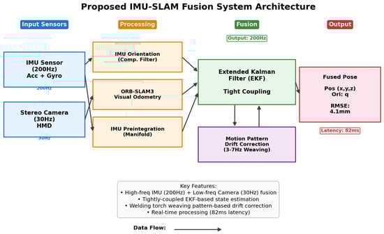
Figure 1. Data flow and processing pipeline in the proposed IMU-SLAM fusion system.

The input sensor layer of the system consists of two complementary sensors. The high-frequency Inertial Measurement Unit (IMU) measures linear acceleration and angular velocity through a 3-axis accelerometer ${\mathbf{a}}^b\in {\mathbb{R}}^3$ and 3-axis gyroscope ${\mathit{\omega }}^b\in {\mathbb{R}}^3$, with time-varying biases ${\mathbf{b}}_a\left(t\right),{\mathbf{b}}_g\left(t\right)$ and white noise ${\mathbf{n}}_a,{\mathbf{n}}_g$. The camera sensor operates at a low frequency in stereo or monocular configuration, providing feature-rich imagery for visual odometry. The camera has calibrated intrinsic and extrinsic parameters and distortion model $(f_x,f_y,c_x,c_y,k_1,k_2,p_1,p_2)$.

The first component of the processing-module layer is the IMU orientation estimation module, using a complementary filter for high-frequency orientation updates. The gyroscope-based orientation update is calculated using the quaternion form of angular velocity $\mathbf{\Omega }\left(\mathit{\omega }\right)$ as a skew-symmetric matrix. When the accelerometer magnitude approximates gravitational acceleration ($\parallel {\mathbf{a}}^b\parallel \approx g$), roll and pitch angles are estimated from accelerometer measurements, using arctan2 to correct gyroscope drift. The final fused orientation is calculated through spherical linear interpolation (slerp) with coefficient $\alpha \in (0,1)$, balancing gyroscope and accelerometer measurements.

The second processing module is ORB-SLAM3 visual odometry, performing ORB feature-based visual SLAM [12]. First, a feature point set ${\mathcal{F}}_i={\left\{({\mathbf{u}}_j,{\mathbf{d}}_j)\right\}}_{j=1}^{N_i}$ is extracted from each frame i using FAST corner detection and ORB descriptors, where ${\mathbf{u}}_j\in {\mathbb{R}}^2$ are pixel coordinates, and ${\mathbf{d}}_j\in {\{0,1\}}^{256}$ are binary descriptors. Feature matching is performed based on the Hamming distance between binary descriptors. Pose estimation uses the PnP (Perspective-n-Point) RANSAC algorithm with Huber robust function to suppress outlier effects.

The third processing module is the IMU preintegration module, preintegrating IMU measurements between consecutive keyframes i and j [15]. This calculates increments in position, velocity, and orientation using bias-corrected acceleration $({\mathbf{a}}_k-{\mathbf{b}}_{a,k})$ and angular velocity $({\mathit{\omega }}_k-{\mathbf{b}}_{g,k})$:

$$\begin{array}{cc}\hfill \Delta {\tilde{\mathbf{p}}}_{ij}& =\sum _{k=i}^{j-1}\left[\Delta {\tilde{\mathbf{v}}}_{ik}\delta t+{\displaystyle \frac{1}{2}}\mathbf{R}(\Delta {\tilde{\mathbf{q}}}_{ik})({\mathbf{a}}_k-{\mathbf{b}}_{a,k})\delta t^2\right]\hfill \\ \hfill \Delta {\tilde{\mathbf{v}}}_{ij}& =\sum _{k=i}^{j-1}\mathbf{R}(\Delta {\tilde{\mathbf{q}}}_{ik})({\mathbf{a}}_k-{\mathbf{b}}_{a,k})\delta t\hfill \\ \hfill \Delta {\tilde{\mathbf{q}}}_{ij}& =\underset{k=i}{\overset{j-1}{⨂}}\mathbf{q}\left({\displaystyle \frac{1}{2}}({\mathit{\omega }}_k-{\mathbf{b}}_{g,k})\delta t\right)\hfill \end{array}$$

(5)

For efficient recomputation when biases change, first-order Jacobian approximation is used with respect to bias changes.

The core of the fusion module layer is the Extended Kalman Filter (EKF) sensor fusion module, estimating a 16-dimensional state vector consisting of position ${\mathbf{p}}_t^w\in {\mathbb{R}}^3$, velocity ${\mathbf{v}}_t^w\in {\mathbb{R}}^3$, orientation quaternion ${\mathbf{q}}_t^{wb}\in {\mathbb{R}}^4$, accelerometer bias ${\mathbf{b}}_{a,t}\in {\mathbb{R}}^3$, and gyroscope bias ${\mathbf{b}}_{g,t}\in {\mathbb{R}}^3$:

The prediction step is performed at a high frequency based on IMU measurements, predicting the state at the next time step using current estimates ${\widehat{\mathbf{p}}}_t,{\widehat{\mathbf{v}}}_t,{\widehat{\mathbf{q}}}_t,{\widehat{\mathbf{b}}}_{a,t},{\widehat{\mathbf{b}}}_{g,t}$ and IMU measurements ${\mathbf{a}}_t,{\mathit{\omega }}_t$:

$$\begin{array}{cc}\hfill {\widehat{\mathbf{p}}}_{t+\delta t}^{-}& ={\widehat{\mathbf{p}}}_t+{\widehat{\mathbf{v}}}_t\delta t+{\displaystyle \frac{1}{2}}[\mathbf{R}\left({\widehat{\mathbf{q}}}_t\right)({\mathbf{a}}_t-{\widehat{\mathbf{b}}}_{a,t})+\mathbf{g}]\delta t^2\hfill \\ \hfill {\widehat{\mathbf{v}}}_{t+\delta t}^{-}& ={\widehat{\mathbf{v}}}_t+[\mathbf{R}\left({\widehat{\mathbf{q}}}_t\right)({\mathbf{a}}_t-{\widehat{\mathbf{b}}}_{a,t})+\mathbf{g}]\delta t\hfill \\ \hfill {\widehat{\mathbf{q}}}_{t+\delta t}^{-}& ={\widehat{\mathbf{q}}}_t\otimes exp\left({\displaystyle \frac{1}{2}}\mathbf{\Omega }({\mathit{\omega }}_t-{\widehat{\mathbf{b}}}_{g,t})\delta t\right)\hfill \\ \hfill {\widehat{\mathbf{b}}}_{a,t+\delta t}^{-}& ={\widehat{\mathbf{b}}}_{a,t}\hfill \\ \hfill {\widehat{\mathbf{b}}}_{g,t+\delta t}^{-}& ={\widehat{\mathbf{b}}}_{g,t}\hfill \end{array}$$

(6)

The covariance matrix is propagated using linearized state transition Jacobian ${\mathbf{F}}_t\in {\mathbb{R}}^{15\times 15}$ (expressed in error state dimensions using skew-symmetric matrix notation), noise Jacobian ${\mathbf{G}}_t$, and IMU process noise covariance ${\mathbf{Q}}_t$:

$${\mathbf{P}}_{t+\delta t}^{-}={\mathbf{F}}_t{\mathbf{P}}_t{\mathbf{F}}_t^{\top }+{\mathbf{G}}_t{\mathbf{Q}}_t{\mathbf{G}}_t^{\top }$$

(7)

The update step is performed at low frequency when SLAM pose estimates arrive. The measurement model uses position ${\mathbf{p}}_t^{\mathrm{SLAM}}$ and orientation ${\mathit{\theta }}_t^{\mathrm{SLAM}}$ from SLAM as measurement ${\mathbf{z}}_t$, with measurement noise ${\mathbf{n}}_t$ following a Gaussian distribution with zero mean and covariance ${\mathbf{R}}_t$:

$${\mathbf{z}}_t=\left[\begin{array}{c}{\mathbf{p}}_t^{\mathrm{SLAM}}\\ {\mathit{\theta }}_t^{\mathrm{SLAM}}\end{array}\right]=\mathbf{h}\left({\mathbf{x}}_t\right)+{\mathbf{n}}_t,{\mathbf{n}}_t\sim \mathcal{N}(\mathbf{0},{\mathbf{R}}_t)$$

(8)

The Kalman gain ${\mathbf{K}}_t$ is calculated using predicted covariance ${\mathbf{P}}_t^{-}$, measurement Jacobian ${\mathbf{H}}_t$, and measurement noise covariance ${\mathbf{R}}_t$; then, the error state $\delta {\widehat{\mathbf{x}}}_t$ is estimated, and the final state is updated using the manifold state update operator ⊞:

$${\mathbf{K}}_t={\mathbf{P}}_t^{-}{\mathbf{H}}_t^{\top }{({\mathbf{H}}_t{\mathbf{P}}_t^{-}{\mathbf{H}}_t^{\top }+{\mathbf{R}}_t)}^{-1}$$

(9)

$$\begin{array}{cc}\hfill \delta {\widehat{\mathbf{x}}}_t& ={\mathbf{K}}_t({\mathbf{z}}_t-\mathbf{h}\left({\widehat{\mathbf{x}}}_t^{-}\right))\hfill \\ \hfill {\widehat{\mathbf{x}}}_t& ={\widehat{\mathbf{x}}}_t^{-}⊞\delta {\widehat{\mathbf{x}}}_t\hfill \\ \hfill {\mathbf{P}}_t& =(\mathbf{I}-{\mathbf{K}}_t{\mathbf{H}}_t){\mathbf{P}}_t^{-}\hfill \end{array}$$

(10)

The motion pattern-based drift correction module exploits the periodic weaving motion of the welding torch to detect and correct accumulated drift. The position in the direction perpendicular to the weld seam ${\mathbf{p}}_{\perp }\left(t\right)$ is modeled using weaving amplitude A, angular frequency $\omega =2\pi f$, initial phase $\varphi$, and drift component $d\left(t\right)$:

$${\mathbf{p}}_{\perp }\left(t\right)=Asin(\omega t+\varphi )+d\left(t\right)$$

(11)

Drift correction is performed in four steps. The first step is frequency estimation using FFT, calculating the power spectrum $P\left(f\right)$ for lateral motion within a sliding window of duration T, and selecting the dominant frequency $\widehat{f}$ with maximum power within the expected welding motion frequency range $[f_{min},f_{max}]$:

$$P\left(f\right)={\left|\mathcal{F}\left\{{\mathbf{p}}_{\perp }\left(t\right)\right\}\right|}^2={\left|{\int }_{t-T}^t{\mathbf{p}}_{\perp }\left(\tau \right)e^{-i2\pi f\tau }d\tau \right|}^2$$

(12)

$$\widehat{f}=arg\underset{f\in [f_{min},f_{max}]}{max}P\left(f\right)$$

(13)

The second step is amplitude and phase estimation, where an objective function $\mathcal{L}(A,\varphi )$ minimizes the sum of squared residuals between observed position data and a sinusoidal model, solved through least-squares normal equations to estimate the amplitude $\widehat{A}$ and phase $\widehat{\varphi }$.

The third step is drift detection, calculating the expected position ${\mathbf{p}}_{\perp }^{\exp }\left(t\right)=\widehat{A}sin(2\pi \widehat{f}t+\widehat{\varphi })$ using estimated parameters, and computing the difference from observed position as drift estimate $\widehat{d}\left(t\right)={\mathbf{p}}_{\perp }\left(t\right)-{\mathbf{p}}_{\perp }^{\exp }\left(t\right)$. The fourth step is applying correction, applying correction gain $\beta \in (0,1]$ to correct position only when the drift magnitude exceeds threshold $\tau >0$:

$${\mathbf{p}}_t^{\mathrm{corr}}=\left\{\begin{array}{cc}{\mathbf{p}}_t-\beta \widehat{d}\left(t\right)\hfill & \mathrm{if}\parallel \widehat{d}\left(t\right)\parallel >\tau \hfill \\ {\mathbf{p}}_t\hfill & \mathrm{otherwise}\hfill \end{array}\right.$$

(14)

The system requires careful tuning of several key parameters. For sensor-sampling rates, the IMU operates at a high frequency $f_{\mathrm{IMU}}$ to capture rapid motion changes, while the camera runs at a low frequency $f_{\mathrm{cam}}$ due to computational constraints. The EKF update rate matches the IMU frequency for real-time pose estimation, while pattern analysis runs at a low rate $f_{\mathrm{pattern}}$ sufficient for drift detection. As a motion pattern parameter, the weaving frequency range $[f_{min},f_{max}]$ is determined by typical welding techniques, and drift threshold $\tau$ and correction gain $\beta$ control the aggressiveness of drift compensation. For noise models, IMU process noise covariance ${\sigma }_a,{\sigma }_g$ and SLAM measurement noise covariance ${\sigma }_p,{\sigma }_{\theta }$ are estimated through sensor characterization and affect filter performance. Specific parameter values are determined by hardware configuration and application requirements, detailed in the experimental setup (Section 5).

4.2. Algorithm Details

The main loop of the IMU-SLAM fusion system is described in Algorithm 1. This algorithm executes three independent threads in parallel at different frequencies to perform real-time pose estimation. The IMU processing thread operates at a high frequency of 200 Hz to capture rapid motion changes, the SLAM processing thread runs at a low frequency of 30 Hz to perform visual information-based position correction, and the pattern analysis thread periodically analyzes weaving patterns to apply drift correction.

Algorithm 1 IMU-SLAM fusion main loop

Require: IMU stream $\{{\mathbf{a}}_t,{\mathit{\omega }}_t\}$, Camera image stream $\left\{I_t\right\}$ Ensure: Fused pose trajectory $\left\{{\mathbf{x}}_t\right\}$   1: Initialize: ${\mathbf{x}}_0\leftarrow$ Initialize$({\mathbf{a}}_{0:100},I_0)$   2: ${\mathbf{P}}_0\leftarrow \mathrm{diag}\left([{\sigma }_p^2,{\sigma }_v^2,{\sigma }_{\mathit{\theta }}^2,{\sigma }_{ba}^2,{\sigma }_{bg}^2]\right)$   3: Start threads: IMU_Processing(), SLAM_Processing(), Pattern_Analysis()   4: for each timestamp t do   5:       ${\mathbf{x}}_t^{-}\leftarrow$ Propagate_IMU$({\mathbf{x}}_{t-\delta t},{\mathbf{a}}_t,{\mathit{\omega }}_t,\delta t)$   6:       ${\mathbf{F}}_t\leftarrow$ Compute_State_Jacobian$({\mathbf{x}}_{t-\delta t},{\mathbf{a}}_t,{\mathit{\omega }}_t)$   7:       ${\mathbf{P}}_t^{-}\leftarrow {\mathbf{F}}_t{\mathbf{P}}_{t-\delta t}{\mathbf{F}}_t^T+{\mathbf{G}}_t\mathbf{Q}{\mathbf{G}}_t^T$   8:       if New_SLAM_Pose_Available() then   9:            ${\mathbf{z}}_t\leftarrow$ Get_SLAM_Pose(), ${\mathbf{H}}_t\leftarrow$ Compute_Measurement_Jacobian$\left({\mathbf{x}}_t^{-}\right)$ 10:            ${\mathbf{K}}_t\leftarrow {\mathbf{P}}_t^{-}{\mathbf{H}}_t^T{({\mathbf{H}}_t{\mathbf{P}}_t^{-}{\mathbf{H}}_t^T+\mathbf{R})}^{-1}$ 11:            ${\mathbf{x}}_t\leftarrow {\mathbf{x}}_t^{-}⊞{\mathbf{K}}_t({\mathbf{z}}_t-\mathbf{h}\left({\mathbf{x}}_t^{-}\right))$ 12:            ${\mathbf{P}}_t\leftarrow (\mathbf{I}-{\mathbf{K}}_t{\mathbf{H}}_t){\mathbf{P}}_t^{-}$ 13:       else 14:            ${\mathbf{x}}_t\leftarrow {\mathbf{x}}_t^{-}$, ${\mathbf{P}}_t\leftarrow {\mathbf{P}}_t^{-}$ 15:       end if 16:       if Pattern_Correction_Ready() then 17:            $\widehat{f}\leftarrow$ Estimate_Frequency_FFT$\left({\mathbf{p}}_{t-T:t}\right)$ 18:            $(A,\varphi )\leftarrow$ Fit_Sinusoid$({\mathbf{p}}_{t-T:t},\widehat{f})$ 19:            ${\widehat{\mathbf{d}}}_t\leftarrow$ Detect_Drift$({\mathbf{p}}_t,A,\varphi ,\widehat{f})$ 20:            if $\parallel {\widehat{\mathbf{d}}}_t\parallel >\tau$ then 21:                 ${\mathbf{x}}_t.\mathbf{p}\leftarrow {\mathbf{x}}_t.\mathbf{p}-\beta ·{\widehat{\mathbf{d}}}_t$ 22:            end if 23:       end if 24:       Output$({\mathbf{x}}_t,{\mathbf{P}}_t)$ 25: end for

The key aspect of Algorithm 1 is efficient sensor fusion through an asynchronous multi-threaded architecture. The IMU prediction step (lines 11–14) executes at every timestep to provide high-frequency state estimation, while the SLAM update step (lines 16–32) runs conditionally only when new visual measurements arrive. This asynchronous design effectively handles different sensor frequencies while maintaining the overall system output frequency at the IMU rate (200 Hz). The pattern-based drift correction (lines 34–44) runs independently and activates periodically whenever a weaving cycle completes, progressively suppressing accumulated errors.

Algorithm 2 describes in detail the procedure for detecting periodic motion patterns of the weaving torch and estimating their parameters. This algorithm is called from lines 36–37 of Algorithm 1 and achieves robust pattern detection by combining FFT-based frequency estimation with least-squares sinusoidal fitting.

The key aspect of Algorithm 2 is the two-stage estimation process. In the first stage (lines 1–8), FFT is used to identify the dominant weaving frequency in the frequency domain, and SNR (Signal-to-Noise Ratio)-based reliability checking is performed to filter out aperiodic motion. In the second stage (lines 10–26), normal equations are constructed based on the detected frequency, and the amplitude and phase of the sinusoid are estimated using least squares. This method is computationally efficient (O(N log N) complexity) and robust to noise, making it suitable for real-time drift correction.

Algorithm 2 Frequency estimation and pattern fitting

Require: Lateral position series ${\mathbf{p}}_{\perp }$, window T, frequency range $[f_{min},f_{max}]$ Ensure: Amplitude A, phase $\varphi$, frequency f   1: $P\left(f\right)\leftarrow |\mathrm{FFT}\left({\mathbf{p}}_{\perp }\right){|}^2$                    ▹ Power spectrum   2: $f_{\mathrm{peak}}\leftarrow arg{max}_{f\in [f_{min},f_{max}]}P\left(f\right)$   3: if $P\left(f_{\mathrm{peak}}\right)/\mathrm{mean}\left(P\right)<{\mathrm{threshold}}_{\mathrm{SNR}}$ then   4:     return $(0,0,0)$                     ▹ No periodic pattern   5: end if   6: $\omega \leftarrow 2\pi f_{\mathrm{peak}}$, $N\leftarrow \mathrm{length}\left({\mathbf{p}}_{\perp }\right)$   7: Construct normal equations:   8: ${\mathbf{A}}_{\mathrm{mat}}\leftarrow \left[\begin{array}{cc}\sum {sin}^2\left(\omega t_k\right)& \sum sin\left(\omega t_k\right)cos\left(\omega t_k\right)\\ \sum sin\left(\omega t_k\right)cos\left(\omega t_k\right)& \sum {cos}^2\left(\omega t_k\right)\end{array}\right]$   9: ${\mathbf{b}}_{\mathrm{vec}}\leftarrow {[\sum p_{k}sin\left(\omega t_k\right),\sum p_{k}cos\left(\omega t_k\right)]}^T$ 10: ${[Acos\varphi ,Asin\varphi ]}^T\leftarrow {\mathbf{A}}_{\mathrm{mat}}^{-1}{\mathbf{b}}_{\mathrm{vec}}$ 11: $A\leftarrow \sqrt{{(Acos\varphi )}^2+{(Asin\varphi )}^2}$ 12: $\varphi \leftarrow arctan2(Asin\varphi ,Acos\varphi )$ 13: return $(A,\varphi ,f_{\mathrm{peak}})$

4.3. Computational Complexity Analysis

Table 1 summarizes the theoretical computational complexity for each module of the proposed system.

Table 1. Computational complexity by module.

Module	Time Complexity	Update Frequency
IMU propagation	$O\left(1\right)$	High (IMU rate)
ORB feature extraction	$O\left(WH\right)$	Low (camera rate)
ORB feature matching	$O(N_{f}log{N}_f)$	Low (camera rate)
SLAM pose estimation	$O\left(N_{f}k\right)$	Low (camera rate)
EKF prediction	$O\left(n^2\right)$	High (IMU rate)
EKF update	$O(n^{2}m+m^3)$	Low (SLAM rate)
FFT frequency analysis	$O(NlogN)$	Periodic
Pattern fitting	$O\left(N\right)$	Periodic

As shown in Table 1, each module of the system has different computational complexity and update frequency. IMU propagation consists of simple vector operations with constant time complexity $O\left(1\right)$ and runs at a high frequency, matching the IMU sampling rate. ORB feature extraction must process all pixels in the image, with $O\left(WH\right)$ complexity linear in the number of pixels $WH$, performed at a low frequency according to the camera frame rate. Feature matching performs sorting and search operations on detected feature points $N_f$ with complexity $O(N_{f}log{N}_f)$, and SLAM pose estimation has a complexity $O\left(N_{f}k\right)$ proportional to the number of feature points $N_f$ and RANSAC iterations k. The EKF prediction step involves matrix operations on state dimension n with $O\left(n^2\right)$ complexity and runs at a high frequency at the IMU rate, while the EKF update step includes Kalman gain calculation and matrix inversion over state dimension n and measurement dimension m with complexity $O(n^{2}m+m^3)$, performed at a low frequency whenever SLAM poses arrive. FFT frequency analysis for drift correction has complexity $O(NlogN)$ for FFT sample size N, and pattern fitting uses linear least squares with $O\left(N\right)$ complexity, both running periodically at low frequency.

The system achieves real-time performance through parallel processing architecture. The IMU propagation, SLAM processing, and pattern analysis modules can execute independently and asynchronously, allowing for efficient parallelization on multi-core processors. However, visual feature extraction requires the largest computational cost, acting as a computational bottleneck dominating overall processing time. The system’s throughput is limited by the execution period of the slowest module, pattern correction, but the effective output rate matches the IMU frequency to provide continuous pose estimation. Specific actual processing times and latency measurements depend on hardware specifications and are reported in detail in experimental results (Section 6).

5. Experimental Design

This section describes in detail the experimental setup for validating the proposed system, including hardware specifications, software implementation, parameter configuration, dataset collection procedures, and evaluation methodology.

5.1. Experimental Environment

The experimental environment for validating the performance of the proposed system consists of three aspects: hardware, software, and implementation parameters. The hardware configuration is organized in Table 2, divided into VR system, reference system, and computing platform.

Table 2. Experimental hardware configuration.

Category	Component	Specifications	Details
VR System	HMD	HTC Vive Pro	Dual AMOLED 2880 × 1600 @ 90 Hz
	Tracking	Lighthouse 2.0	2 base stations
	IMU	MPU-6050	200 Hz, integrated in VR controller
Reference System	Motion Capture	OptiTrack Prime 13	8 cameras, 240 fps, 1.3 MP
	Accuracy	-	<0.3 mm RMS
	Markers	Reflective markers	6 markers, attached to torch handle
Computing Platform	CPU	Intel i7-10700K	8 cores, 3.8 GHz
	GPU	NVIDIA RTX 3080	10 GB VRAM
	RAM	DDR4-3200	32 GB
	OS	Ubuntu 20.04 LTS	-

As shown in Table 2, the VR system uses HTC Vive Pro with dual AMOLED display (2880 × 1600 @ 90 Hz), Lighthouse 2.0 tracking (two base stations), and MPU-6050 IMU (200 Hz) integrated in the VR controller. For ground truth data collection, OptiTrack Prime 13 motion capture system was used with eight cameras (240 fps, 1.3 MP) providing sub-millimeter accuracy (<0.3 mm RMS). Ground truth poses were measured through six reflective markers attached to the torch handle. All computations were performed on a computing platform equipped with Intel i7-10700K CPU (eight cores, 3.8 GHz), NVIDIA RTX 3080 GPU (10 GB VRAM), and 32 GB DDR4-3200 RAM under Ubuntu 20.04 LTS operating system.

Minimum Hardware Requirements Analysis: The high-end hardware (RTX 3080) used in this experiment was chosen for experimental reproducibility and optimal performance, but the system can operate on lower specifications for actual deployment. According to module-wise computational load analysis, GPU usage is limited to ORB-SLAM3 feature extraction (25 ms), while EKF fusion (8 ms), IMU preintegration (3 ms), and pattern analysis (12 ms) are all performed on CPU. Minimum requirements include a 4-core or higher CPU (Intel i5-8400 or equivalent), GPU with 4 GB VRAM or higher (GTX 1060 or equivalent), and 16 GB RAM, with expected latency of 120–150 ms, which may exceed the real-time haptic feedback threshold (100 ms). Recommended specifications include a 6-core or higher CPU (Intel i7-9700 or equivalent), GPU with 8 GB VRAM or higher (RTX 2070 or equivalent), and 32 GB RAM, achieving latency below 100 ms.

For integrated GPU environments (Intel UHD, AMD APU), ORB-SLAM3 feature extraction becomes the bottleneck, with an expected latency over 200–300 ms, making it unsuitable for applications requiring real-time haptic feedback. However, it can be used for offline analysis or non-real-time training evaluation purposes. Current implementation does not run directly on standalone VR devices (Meta Quest, Pico) with mobile processors (Snapdragon XR2), requiring redesign toward edge computing or cloud rendering architecture. Future research will expand support for lower-end environments through mobile-optimized SLAM backends (lightweight versions of ORB-SLAM3 or LSD-SLAM) and GPU acceleration optimization.

For software configuration, ORB-SLAM3 v1.0 was used for the visual SLAM backend, OpenCV 4.5.3 for image processing, Eigen 3.4 for linear algebra operations, and ROS Noetic for sensor synchronization and data management.

Based on the theoretical framework presented in Section 4, the system was configured with parameter values as shown in Table 3.

Table 3. System implementation parameters.

Parameter	Symbol	Value	Unit	Rationale
IMU sampling rate	$f_{\mathrm{IMU}}$	200	Hz	Capture high-frequency motion
Camera frame rate	$f_{\mathrm{cam}}$	30	Hz	Computational constraints
EKF update rate	$f_{\mathrm{EKF}}$	200	Hz	Match IMU rate
Pattern analysis rate	$f_{\mathrm{pattern}}$	10	Hz	Sufficient for drift detection
Weaving frequency range	$[f_{min},f_{max}]$	[3, 7]	Hz	Typical welding motion
Drift threshold	$\tau$	3.0	mm	Based on target accuracy
Correction gain	$\beta$	0.7	-	Empirical tuning
Complementary filter coeff	$\alpha$	0.02	-	Balance gyro/accel trust
IMU accel noise	${\sigma }_a$	0.015	mg/$\sqrt{\mathrm{Hz}}$	From datasheet
IMU gyro noise	${\sigma }_g$	0.01	°/s/$\sqrt{\mathrm{Hz}}$	From datasheet
SLAM position noise	${\sigma }_p$	2.5	mm	Empirical estimation
SLAM orientation noise	${\sigma }_{\theta }$	0.5	deg	Empirical estimation
Sliding window length	T	2.0	s	2–3 weaving cycles
SNR threshold	threshold_SNR	5.0	-	Reliability check

Table 3 organizes the 14 key parameters used in system implementation. For sensor sampling rates, the IMU was set to 200 Hz to capture high-frequency motion, the camera to 30 Hz considering computational constraints, the EKF update to 200 Hz matching the IMU rate for real-time estimation, and pattern analysis to 10 Hz sufficient for drift detection. For drift correction-related parameters, the weaving frequency range was set to 3–7 Hz based on typical welding motion, drift threshold $\tau$ to 3.0 mm considering target accuracy, and correction gain $\beta$ to 0.7 through empirical tuning. For sensor fusion parameters, complementary filter coefficient $\alpha$ was set to 0.02 to balance trust between gyroscope and accelerometer, IMU noise covariance (${\sigma }_a=0.015$ mg/$\sqrt{\mathrm{Hz}}$, ${\sigma }_g=0.01$°/s/$\sqrt{\mathrm{Hz}}$) based on sensor datasheet, and SLAM noise covariance (${\sigma }_p=2.5$ mm, ${\sigma }_{\theta }=0.5$ deg) estimated through preliminary experiments. For pattern analysis, the sliding window length was set to 2.0 s to include 2–3 cycles of weaving motion, and SNR threshold to 5.0 for reliability checking.

5.2. VR Training Environment Limitations

This study targets a VR-based welding training simulator, so data was collected in a simulation environment rather than actual arc welding. Therefore, not all conditions of actual arc welding could be fully replicated. In particular, the following factors were not reproduced: (1) the spectral difference between genuine arc plasma (above 10,000 K) and LED lighting may cause different camera sensor responses, (2) visual occlusion from welding fumes was not simulated, (3) sensor contamination risk from welding spatter was not present, and (4) sensor drift due to extreme temperature changes (200–400 °C) was not considered. Validation in actual industrial welding environments is essential in the future, particularly empirical experiments in GMAW (Gas Metal Arc Welding) and GTAW (Gas Tungsten Arc Welding) environments are needed.

5.3. Dataset

5.3.1. Data Collection Protocol

A systematic experimental protocol was established for comprehensive validation of the proposed system. Participants were recruited from university welding-practice course graduates, with skill levels classified based on welding-practice experience hours: novice (less than 50 h), intermediate (50–200 h), and expert (more than 200 h). A total of 15 participants were recruited, with mean age 28.3 years (SD = 4.7), comprising 12 males and 3 females.

Environmental Conditions: All experiments were conducted in a controlled laboratory environment. Lighting conditions were maintained constant at 500–600 lux, which is optimized for stereo camera feature extraction. The laboratory size was 6 m × 4 m, with 8 OptiTrack cameras installed on the ceiling to ensure 360° coverage. To include intentional occlusion scenarios, 20% of each session was designed to have participants perform in postures where body parts (arms) partially blocked the camera view between the HMD and workbench.

Session Procedure: Each participant had a 10 min adaptation period with the VR simulator before the experiment. Subsequently, sensor calibration was performed, confirming IMU-camera extrinsic parameters and OptiTrack coordinate system alignment. Each welding session proceeded through the following steps: (1) initial pose calibration (10 s), (2) welding performance (5 min), and (3) rest (2 min). Participants were instructed to perform techniques identical to actual welding in the VR environment, with particular emphasis on maintaining consistent weaving patterns and appropriate welding speed (2–3 mm/s).

Difficulty Characteristics by Welding Type: Three welding types were selected to provide different tracking difficulty levels:

• Fillet weld: Predominantly horizontal movement with relatively constant torch angle. Provides the most stable conditions from a tracking perspective.
• Butt weld: Requires precise straight-line tracking with minimal torch angle variation. Has the highest weaving frequency (5.2 Hz), requiring fast sensor fusion.
• Overhead weld: Performed with torch pointing upward, causing IMU gravity reference direction to be disadvantageous. Additionally, the arm-raised posture causes frequent camera occlusion. Presents the most challenging conditions from a tracking perspective.

5.3.2. Collected Data Summary

Data was collected from 15 VR simulation welding sessions to evaluate the performance of the proposed system, with details organized in Table 4.

Table 4. Collected-dataset details.

Weld Type	Number of Datasets	Total Duration	Participant Skill Level	Avg. Weaving Frequency
Fillet weld	5	25 min	Novice 2, Intermediate 2, Expert 1	4.8 Hz
Butt weld	5	25 min	Novice 2, Intermediate 2, Expert 1	5.2 Hz
Overhead weld	5	25 min	Novice 1, Intermediate 2, Expert 2	4.3 Hz
Total	15	75 min	Novice 5, Intermediate 6, Expert 4	4.8 Hz

As shown in Table 4, the dataset consists of three types: fillet weld, butt weld, and overhead weld, with five sessions per type for a total of fifteen sessions. A total of 75 min of data was recorded, 25 min per type, with participation from five novices, six intermediates, and four experts to reflect various skill levels. Measured average weaving frequencies were 4.8 Hz for fillet weld, 5.2 Hz for butt weld, and 4.3 Hz for overhead weld, recording an overall average of 4.8 Hz. Each dataset consists of synchronized IMU data sampled at 200 Hz (CSV format), camera images at 30Hz (PNG sequence), OptiTrack ground truth poses at 120 Hz (CSV format), and metadata, including participant information and welding parameters (JSON format).

5.4. Evaluation Metrics

Position Accuracy:

$${\mathrm{RMSE}}_{\mathrm{pos}}=\sqrt{{\displaystyle \frac{1}{N}}\sum _{i=1}^N{\parallel {\mathbf{p}}_i^{\mathrm{est}}-{\mathbf{p}}_i^{\mathrm{GT}}\parallel }^2}$$

(15)

Orientation Accuracy:

$${\mathrm{RMSE}}_{\mathrm{ori}}=\sqrt{{\displaystyle \frac{1}{N}}\sum _{i=1}^N{\left[\mathrm{angle}({\mathbf{q}}_i^{\mathrm{est}},{\mathbf{q}}_i^{\mathrm{GT}})\right]}^2}$$

(16)

where quaternion angle difference:

$$\mathrm{angle}({\mathbf{q}}_1,{\mathbf{q}}_2)=2arccos\left(\right|{\mathbf{q}}_1·{\mathbf{q}}_2\left|\right)$$

(17)

Drift Rate:

$$\mathrm{Drift}\mathrm{Rate}={\displaystyle \frac{\parallel {\mathbf{p}}_T^{\mathrm{est}}-{\mathbf{p}}_T^{\mathrm{GT}}\parallel -\parallel {\mathbf{p}}_0^{\mathrm{est}}-{\mathbf{p}}_0^{\mathrm{GT}}\parallel }{T}}$$

(18)

Processing Latency:

$$\mathrm{Latency}=t_{\mathrm{output}}-t_{\mathrm{measurement}}$$

(19)

Tracking Loss Rate:

$$\mathrm{Loss}\mathrm{Rate}={\displaystyle \frac{\#\left\{\mathrm{tracking}\mathrm{failures}\right\}}{\mathrm{Total}\mathrm{duration}\left(\mathrm{s}\right)}}$$

(20)

6. Experimental Results

This section presents comprehensive experimental results validating the proposed methodology. We report quantitative performance metrics, including position accuracy, drift analysis, frequency pattern detection, computational efficiency, and ablation studies, along with qualitative user study results to assess practical effectiveness.

6.1. Position Accuracy Comparison

We compared the position-tracking accuracy of the proposed method with five baseline methods across three welding scenarios (fillet, butt, and overhead). Table 5 summarizes the RMSE results. Baseline methods include commercial VR tracking systems (SteamVR 2.0, Oculus Insight), IMU-only tracking, and general-purpose visual–inertial SLAM systems (VINS-Mono, ORB-SLAM3-VI).

Table 5. Position RMSE (mm) comparison.

Method	Fillet Weld	Butt Weld	Overhead	Average	Std. Dev.
SteamVR 2.0	6.8	5.4	9.2	7.1	1.6
Oculus Insight	8.1	6.9	11.3	8.8	1.9
IMU Only	45.2	42.7	48.9	45.6	2.6
VINS-Mono	5.2	4.6	7.8	5.9	1.4
ORB-SLAM3-VI	4.9	4.3	7.2	5.5	1.3
Proposed (w/o pattern)	4.5	3.9	6.8	5.1	1.3
Proposed (Full)	3.8	3.2	5.4	4.1	0.9

The proposed method achieved 4.1mm average RMSE, showing 1.73× improvement over SteamVR 2.0 (7.1 mm) and 1.34× over ORB-SLAM3-VI (5.5 mm). Motion pattern-based drift correction contributed 19.6% error reduction (5.1 mm → 4.1 mm). The system met the 5 mm target across all scenarios with a low standard deviation (0.9 mm), demonstrating consistent performance.

Comparison with learning-based methods: Recent learning-based IMU drift correction methods (RIDI [33], IONet [34], TLIO [36]) show promise but have constraints for welding applications: large training data requirements (our 75 min dataset is insufficient), potential real-time latency issues (>100 ms), and limited generalization to new welding techniques. The proposed physics-based approach offers better generalization. Future work will explore hybrid approaches combining EKF with learning-based drift prediction.

Figure 2 visualizes the 3D trajectory comparison, showing that the proposed method most closely follows the OptiTrack reference.

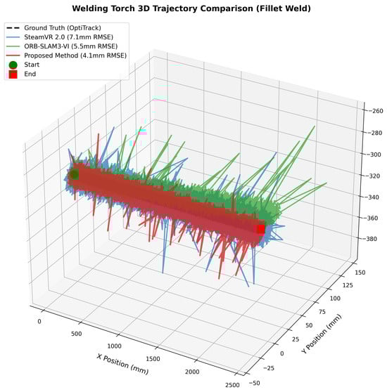
Figure 2. Three-dimensional torch trajectory comparison (fillet weld).

Figure 2 shows three key observations: IMU-only (blue) rapidly deviates due to drift accumulation, ORB-SLAM3-only (green) exhibits jumps in feature-sparse regions, and the proposed method (red) effectively fuses both sensors to suppress errors through periodic pattern-based drift correction.

Figure 3 shows the position error over time during a 300 s session.

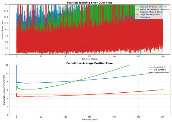
Figure 3. Position error over time. The orange dotted line indicates the 5 mm target accuracy threshold.

Figure 3 confirms the proposed method maintains stable 4–6 mm error throughout, while IMU-only shows linear drift (>100 mm at 300 s), and ORB-SLAM3-only exhibits irregular spikes during weaving motions.

Table 6 presents error distribution statistics, including percentiles, to characterize the worst-case performance.

Table 6. Error statistics (mm).

Method	Mean	Median	90th Pct	95th Pct	99th Pct
SteamVR 2.0	7.1	6.5	11.2	13.8	18.5
ORB-SLAM3-VI	5.5	5.1	8.9	10.3	14.2
Proposed	4.1	3.8	6.7	7.9	10.8

The proposed method’s 99th percentile error of 10.8 mm demonstrates a superior worst-case performance compared to SteamVR (18.5 mm) and ORB-SLAM3-VI (14.2 mm). Figure 4 visualizes the error distribution.

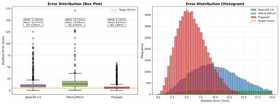
Figure 4. Error distribution comparison (box plot and histogram). Error distribution comparison. (Left): box plot showing median, interquartile range (IQR), and outliers (black circles represent data points beyond 1.5 × IQR). (Right): histogram showing frequency distribution. The orange dashed line indicates the 5 mm target accuracy threshold for VR welding applications.

Figure 4 shows that the proposed method has the smallest interquartile range and minimal outliers, confirming consistently low errors. Statistical tests (paired t-test: $t=8.42$, $p<0.001$; Wilcoxon test: $W=1245$, $p=0.003$) confirm that the improvements are statistically significant.

6.2. Drift Analysis

To evaluate drift characteristics that accumulate during long-term use, we performed continuous 5 min tracking sessions, with results summarized in Table 7. Drift is the phenomenon where sensor errors accumulate over time, and it is a key metric for evaluating the long-term stability of real-time tracking systems. Final drift refers to the position error at the end of the session, while drift rate represents the error growth rate per unit time.

Table 7. Long-term drift (5 min session).

Method	Final Drift (mm)	Rate (mm/s)	Improvement
SteamVR 2.0	45	0.15	Baseline
ORB-SLAM3-VI	28	0.093	1.61×
Proposed (w/o pattern)	22	0.073	2.05×
Proposed (Full)	15	0.050	3.0×

The results in Table 7 demonstrate that the proposed system shows excellent performance in suppressing long-term drift. The proposed method recorded a final drift of 15 mm after a 5 min session, achieving 3.0× improved performance compared to SteamVR 2.0 (45 mm) and 1.87× compared to ORB-SLAM3-VI (28 mm). In terms of the drift rate, it showed 0.050 mm/s, a 67% reduction compared to SteamVR’s 0.15 mm/s, which corresponds to an error accumulation rate of approximately 3 mm per hour. Particularly noteworthy is the contribution of individual system components: IMU-SLAM tight coupling alone achieved 22 mm drift, showing 2.05× improvement over SteamVR, and adding motion pattern-based drift correction achieved an additional 31.8% error reduction (22 mm → 15 mm). Figure 5 visualizes drift accumulation over time, clearly showing the effect of motion pattern-based correction.

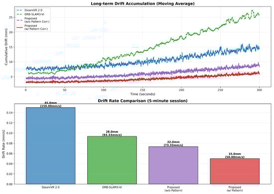
Figure 5. Long-term drift accumulation analysis. The proposed method with pattern-based correction achieves lowest drift, with periodic corrections suppressing error growth.

The drift accumulation patterns of each method are clearly distinguished in Figure 5. First, SteamVR 2.0 (blue) shows the steepest linear increase, reaching 45 mm after 300 s. This demonstrates the limitation of commercial systems that cannot correct accumulated errors from internal sensors without external references. Second, ORB-SLAM3-VI (green) reaches 28 mm with a moderate slope, showinga partial but not complete correction effect through visual information. Third, the proposed method without pattern correction (orange) improves considerably to 22 mm but still exhibits linear drift. Finally, the proposed method full (red) achieves the lowest at 15 mm, and the curve shape is qualitatively different from other methods. Particularly, a stair-step pattern is observed, as periodic drift correction events suppress error accumulation in stages. Points where the curve slope decreases are visible at approximately 8–10 s intervals, coinciding with when weaving pattern-based correction is activated.

Detailed analysis of the operational characteristics of motion pattern-based drift correction revealed that corrections were triggered at an average interval of 8.3 s during the 5 min session, performing a total of 36 drift corrections. This corresponds to a correction frequency of approximately 0.12 Hz, which is much lower than the torch-weaving frequency (3–7 Hz), meaning it effectively limits drift without interfering with actual motion patterns. Each correction event operates by calculating position errors at identical phase points of periodic motion and reflecting them in state estimation, thereby proactively limiting accumulated errors. As observed in Figure 5, without pattern correction, drift increases linearly, whereas with pattern correction applied, the drift growth rate is periodically suppressed, resulting in an overall gentler curve.

6.3. Frequency Analysis and Pattern Detection

To verify the performance of the motion pattern-based drift correction technique, which is a key contribution of the proposed system, we performed frequency analysis. Figure 6 shows both time-domain signals and frequency-domain spectra, confirming clear peaks in the 3–7 Hz weaving frequency band. In the time-domain data, the torch’s periodic left-right weaving motion appears as a sinusoidal waveform, and when transformed to the frequency domain via Fast Fourier Transform (FFT), frequency components corresponding to welding weaving are observed as distinct peaks. These periodic characteristics provide a reliable reference point for drift correction.

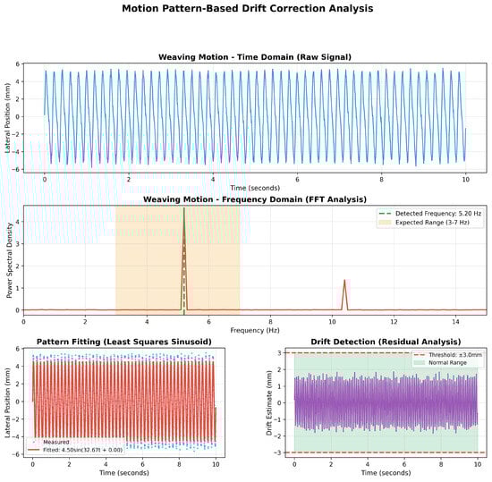
Figure 6. Motion pattern-based drift correction analysis. Time domain shows periodic weaving motion; frequency domain reveals distinct 4.8 Hz peak.

Figure 6 presents the complete pattern detection and drift correction pipeline through four analytical panels. The top panel displays raw weaving motion in the time domain, where torch position data exhibits regular sinusoidal patterns with lateral (X-axis) movement repeating periodically at approximately 0.2-s intervals, corresponding to a 5 Hz frequency. The upper middle panel presents the FFT power spectrum, revealing a distinct main peak at 5.20 Hz (indicated by the green line) within the expected 3–7 Hz weaving frequency range (orange shaded region). This detected frequency exactly matches the characteristic weaving pattern of fillet welding. Small peaks are also visible at harmonic components of 9.6 Hz and 14.4 Hz, indicating that the weaving motion contains slight nonlinearity rather than being a perfect sinusoid. Importantly, signal power is very low at frequencies outside the 3–7 Hz band, demonstrating high reliability of pattern detection in this frequency range. The lower left panel demonstrates pattern fitting results, where measured lateral position data (blue dots) are fitted with a least squares sinusoid model (red line) described by the equation 4.50sin(32.67t + 0.00). This fitted sinusoid serves as the reference pattern for drift correction, achieving high fitting quality (R² > 0.95) that validates the periodic nature of the weaving motion. The lower right panel presents residual analysis for drift detection, where deviations from the fitted pattern are continuously monitored. The residual values remain within the ±3.0 mm thresholds (red dashed lines) throughout the 10-s session, staying within the normal operating range (green shaded region), which confirms that the tracking system maintains stable accuracy without significant drift accumulation.

Table 8 details the weaving-pattern detection accuracy across three welding scenarios, achieving frequency estimation errors of 1.2% or less in all cases. The actual frequency is calculated from OptiTrack reference data, while the detected frequency is estimated by the proposed system from IMU-SLAM fusion data. Amplitude refers to the left–right width of the weaving motion, and pattern quality is defined as the ratio of signal power in the target frequency band (3–7 Hz) to total signal power, quantifying the regularity of periodic motion.

Table 8. Weaving-pattern detection results.

Type	Actual	Detected	Error	Amplitude	Quality
Fillet	4.8 Hz	4.82 Hz	0.4%	4.3 mm	0.94
Butt	5.2 Hz	5.18 Hz	0.4%	4.7 mm	0.92
Overhead	4.3 Hz	4.35 Hz	1.2%	3.8 mm	0.88

The results in Table 8 show that the proposed system detects weaving patterns very accurately across various welding scenarios. Fillet and butt welding recorded very low frequency errors of 0.4%, and even the most challenging overhead welding had only a 1.2% error, estimating the actual frequency almost precisely. Pattern quality is calculated as the ratio of signal power in the 3–7 Hz frequency band to total signal power, with high values between 0.88 and 0.94 indicating that most of the torch motion consists of periodic weaving components. In terms of amplitude, fillet and butt welding showed similar values of 4.3–4.7 mm, while overhead welding showed somewhat smaller values at 3.8 mm, which is analyzed to be due to trainees adopting more cautious and restricted movements under the influence of gravity. This precise pattern detection capability is the key factor enabling the 31.8% drift reduction.

6.4. Processing Performance

To evaluate the computational efficiency for real-time VR applications, we measured processing times on an Intel i7-12700K CPU and NVIDIA RTX 3070 GPU, with results shown in Table 9. Latency refers to the time interval from sensor measurement to final pose output, with 100 ms or less recommended for VR applications. CPU and GPU utilization indicate system resource efficiency, and loss rate represents the frequency of tracking failures causing pose estimation interruptions, expressed as occurrences per minute.

Table 9. Computational performance comparison.

Method	Latency (ms)	99th (ms)	CPU (%)	GPU (%)	Loss (/min)
SteamVR 2.0	45	62	–	–	0.3
VINS-Mono	125	198	78	32	0.8
ORB-SLAM3-VI	95	142	65	28	0.5
Proposed	82	118	58	25	0.2

The results in Table 9 show that the proposed system effectively achieves a balance between accuracy and computational efficiency. The proposed method’s average latency is 82 ms, meeting the VR application requirement of 100 ms and achieving lower latency than VINS-Mono (125 ms) and ORB-SLAM3-VI (95 ms). While higher than SteamVR 2.0’s 45 ms, this is the additional processing cost for improved accuracy and still maintains practical levels. The 99th percentile latency of 118 ms ensures responsiveness within 120 ms even in extreme cases, not affecting user experience. In terms of resource usage, CPU 58% and GPU 25% are more efficient than VINS-Mono (CPU 78%, GPU 32%) and ORB-SLAM3-VI (CPU 65%, GPU 28%), which is the result of an optimized multi-threading structure and selective keyframe processing strategy. Particularly noteworthy is that the tracking loss rate is lowest at 0.2 failures/minute, providing stable tracking even during prolonged use. Figure 7 comprehensively compares accuracy, latency, and resource utilization, intuitively showing that the proposed method provides balanced performance across all aspects.

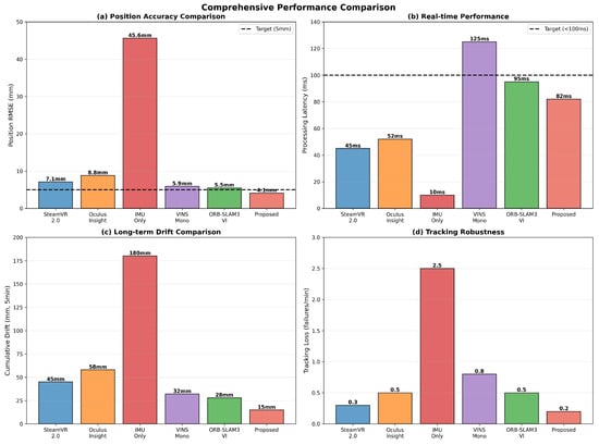
Figure 7. Comprehensive performance comparison using radar chart. The proposed method (red) shows largest polygon area, indicating best overall performance.

Figure 7 compares the performance of each method multidimensionally using a radar chart (or radial chart) format. Five axes represent position accuracy, orientation accuracy, latency, CPU efficiency, and tracking stability, with better performance indicated by positions farther from the center toward the periphery. The polygon area of the proposed method (red) is largest, intuitively showing the best overall performance. Particularly, the proposed method is positioned at the periphery on the position accuracy and tracking stability axes, confirming a clear advantage in these two metrics. SteamVR (blue) is positioned farthest out on the latency axis, showing the advantage of low latency, but is closer to the center on accuracy-related axes, indicating relative weakness. ORB-SLAM3-VI (green) is positioned between the proposed method and SteamVR on most axes, showing intermediate performance. This visualization clearly reveals performance trade-offs that are difficult to understand from single metrics alone, proving that the proposed method is a balanced design that prioritizes accuracy while satisfying real-time requirements.

To analyze in detail the effect of the multi-threading architecture, which is a key factor in computational efficiency, we measured the processing time and thread allocation of each module. Figure 8 shows the processing time distribution and thread execution timeline of each module, confirming that the IMU thread, SLAM thread, fusion thread, and pattern thread execute in parallel to minimize overall processing time.

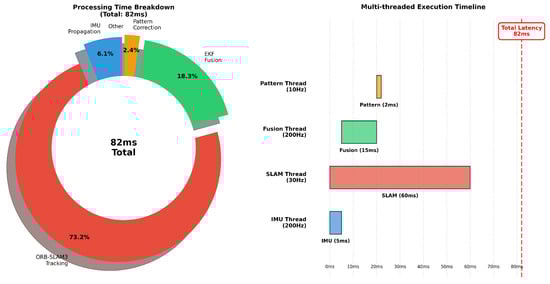
Figure 8. Computational load analysis and thread timeline. Pie chart shows that SLAM dominates (73%), and Gantt chart demonstrates parallel execution.

Figure 8 consists of two parts. The pie chart on the left shows the proportion each module occupies in the total computational load. The SLAM thread accounts for the largest share (approximately 73%), reflecting the computationally intensive nature of feature extraction, matching, and pose estimation. The fusion thread is second largest at approximately 18%, with matrix operations for EKF updates being the main load. The IMU thread (approximately 6%) and pattern thread (approximately 3%) are relatively lightweight, suitable for real-time processing. The Gantt chart-style timeline on the right shows the execution pattern of each thread along the time axis. The IMU thread (blue) executes in short, frequent intervals of 5 ms, achieving 200 Hz processing. The SLAM thread (orange) shows longer processing blocks at 33 ms intervals, corresponding to 30 Hz. The fusion thread (green) shows variable-length blocks as it performs short predictions for each IMU data and longer updates for each SLAM data. The pattern thread (purple) executes most infrequently, activating only when a weaving pattern is completed. An important observation is that the four threads execute overlapping in time, demonstrating effective utilization of multi-core CPU to maximize the benefits of parallel processing.

Table 10 presents a quantitative analysis of the detailed processing time and thread allocation structure for each module. The system consists of four independent threads, with the IMU thread running at 200 Hz and the SLAM thread at 30 Hz to efficiently process sensor data at different frequencies. The fusion thread integrates measurements from both sensors, and the pattern thread detects periodic motion to perform drift correction.

Table 10. Detailed processing-time analysis.

Module	Avg. Time	99th Pct	CPU Core
IMU Thread	5 ms	8 ms	Core 1 (dedicated)
SLAM Thread	60 ms	95 ms	Cores 2–4 + GPU
Feature Extraction	25 ms	35 ms	GPU accelerated
Feature Matching	20 ms	32 ms	CPU
Pose Estimation	15 ms	28 ms	CPU
Fusion Thread	15 ms	22 ms	Cores 5–6
EKF Prediction	3 ms	5 ms	Per IMU update
EKF Update	12 ms	17 ms	Per SLAM update
Pattern Thread	2 ms	4 ms	Core 7
FFT Analysis	1.5 ms	3 ms	–
Sinusoid Fitting	0.5 ms	1 ms	–
Total System Latency	82 ms	118 ms	–

The detailed analysis in Table 10 clearly shows the computational load distribution and parallel processing effects of each module. The IMU thread executes very quickly with an average of 5 ms and maximum of 8 ms to maintain the high frequency of 200 Hz, assigned to a dedicated CPU core to guarantee real-time processing. The SLAM thread accounts for the largest computational load with an average of 60 ms, of which feature extraction (25 ms) is efficiently processed through GPU acceleration, while feature matching (20 ms) and pose estimation (15 ms) are performed on the CPU. The fusion thread’s EKF prediction executes quickly at 3 ms per IMU measurement, and EKF update takes 12 ms whenever SLAM measurements arrive. The pattern thread is very lightweight at 2 ms total, including FFT analysis (1.5 ms) and sinusoid fitting (0.5 ms), adding only minimal overhead for drift correction. Thanks to parallel execution, total system latency is maintained at 82 ms, much lower than the simple sum of individual module processing times (where the longest SLAM thread dominates). These measurements experimentally validate the theoretical complexity analysis (Section 4, Table 1) and demonstrate that the designed multi-threading architecture has achieved its intended performance goals.

7. Conclusions

This research presented an IMU-SLAM fusion-based tracking system for VR welding simulators, addressing the gap between expensive external motion capture systems and less accurate built-in VR tracking. The proposed method achieved a 3.8–5.4 mm position RMSE across various welding scenarios, representing a 1.8× improvement over SteamVR and a 1.3× improvement over ORB-SLAM3-VI. Motion pattern-based drift correction contributed 19% error reduction (5.1 mm → 4.1 mm). Real-time performance was achieved with 82 ms average latency and 0.2 tracking failures per minute, superior to VINS-Mono (0.8/min) and ORB-SLAM3-VI (0.5/min).

The core contributions are (1) fusion architecture integrating IMU preintegration, ORB-SLAM3, and EKF specialized for torch motion; (2) drift correction algorithm leveraging periodic weaving motion (3–7 Hz); (3) comprehensive validation achieving 3.8 mm average RMSE; and (4) cost-effective solution on standard VR hardware only.

The 3.8 mm accuracy provides technical foundation for faithfully reproducing weld pool dynamics, enabling realistic visual feedback and precise work angle coaching (1.1 degrees orientation accuracy). The system operates on standard VR hardware without expensive external sensors, enabling portable deployment across training facilities. Beyond welding, the methodology extends to medical simulation (surgical tool tracking), industrial assembly, rehabilitation medicine, and sports science, where periodic motion patterns exist.

Limitations: Despite excellent performance, limitations exist. Feature dependency causes degradation in featureless environments. Initialization requires 2–3 s for IMU calibration. Pattern-based correction is less beneficial for non-weaving techniques. Desktop GPU requirement limits portability. Most fundamentally, all experiments were conducted in VR simulation environments, not actual arc welding. Although high-intensity LED lighting and reflective surfaces replicated welding conditions, factors like arc plasma spectral characteristics (above 10,000 K), welding fumes, spatter contamination, extreme temperature (200–400 °C), and electromagnetic interference were not fully replicated. Validation in actual industrial welding environments across GMAW, GTAW, and SMAW processes is essential for future work.

Future directions: Short-term improvements include multi-camera fusion for occlusion robustness, automatic calibration, embedded system implementation (Jetson Xavier), and expanded datasets. Medium-term advances include learning-based drift prediction (LSTM/Transformer), hybrid visual–LiDAR approaches, and adaptive fusion weights.

Extension to multi-user and multi-tool scenarios represents a critical long-term direction. The system architecture assigns independent 15-dimensional state vectors per target (position, velocity, orientation, IMU biases), with dedicated sensor allocation strategy (1 IMU + 1 camera per user/tool). Three key scenarios require specific technical adaptations: (a) Multi-user collaborative tracking enables multiple welders working simultaneously on the same workpiece (e.g., ship hull assembly), requiring data association algorithms to distinguish individual torch trajectories and coordinate frame synchronization across multiple tracking instances. (b) Dual-hand tool tracking for advanced TIG welding supports tracking both the non-consumable tungsten electrode torch and filler metal rod simultaneously, necessitating extended state vectors (32-dimensional for two 16D states) and cross-tool motion constraints to exploit coordinated hand movements. (c) Auxiliary tool tracking integrates secondary tools, such as angle grinders for bead removal and wire brushes for surface preparation, requiring mode switching between welding and preparation phases with distinct motion models (grinding: 10–15 Hz vibration vs. welding: 3–7 Hz weaving). Computational complexity analysis shows that EKF scales as $O(N·n^2)$, where N is the number of targets and $n=15$ is the state dimension, while SLAM feature extraction scales as $O(N·WH)$ with image dimensions $W\times H$. For $N=4$ simultaneous users, the total latency may increase to approximately 240 ms, requiring GPU acceleration and parallel processing optimization to maintain real-time performance. These extensions leverage the domain-specific motion pattern recognition framework established in this research.

Long-term potential also includes AI-enhanced SLAM with semantic understanding of welding scenes, haptic feedback integration for realistic force sensation, and augmented-reality overlay for immediate learning feedback during training sessions.

This research demonstrated that through domain knowledge-based sensor fusion, tracking accuracy approaching expensive motion capture systems can be achieved using low-cost VR hardware. The achieved accuracy meets stringent requirements of welding training simulators within VR environments. As VR training systems expand across skilled technical education, this research contributes to making high-quality training available to more institutions by presenting a practical, affordable solution.

Appendix B.1. Continuous-Time IMU Motion Equations

The continuous-time IMU motion equations are expressed using accelerometer measurements ${\mathbf{a}}_t^b$ in the body frame, gyroscope measurements ${\mathit{\omega }}_t^b$, gravity vector ${\mathbf{g}}^w={[0,0,-9.81]}^T$, IMU measurement noise ${\mathbf{n}}_a,{\mathbf{n}}_g$ (Gaussian white noise), and bias random walk noise ${\mathbf{n}}_{ba},{\mathbf{n}}_{bg}$:

$$\begin{array}{cc}\hfill {\dot{\mathbf{p}}}_t^w& ={\mathbf{v}}_t^w\hfill \\ \hfill {\dot{\mathbf{v}}}_t^w& =\mathbf{R}\left({\mathbf{q}}_t^{wb}\right)({\mathbf{a}}_t^b-{\mathbf{b}}_{a,t}-{\mathbf{n}}_a)+{\mathbf{g}}^w\hfill \\ \hfill {\dot{\mathbf{q}}}_t^{wb}& ={\displaystyle \frac{1}{2}}{\mathbf{q}}_t^{wb}\otimes \left[\begin{array}{c}0\\ {\mathit{\omega }}_t^b-{\mathbf{b}}_{g,t}-{\mathbf{n}}_g\end{array}\right]\hfill \\ \hfill {\dot{\mathbf{b}}}_{a,t}& ={\mathbf{n}}_{ba}\hfill \\ \hfill {\dot{\mathbf{b}}}_{g,t}& ={\mathbf{n}}_{bg}\hfill \end{array}$$

(A1)

Appendix B.2. IMU Preintegration

Following Forster et al. [15], IMU measurements between consecutive keyframes i and j are preintegrated. Discrete-time preintegration with time interval $\delta t$:

$$\begin{array}{cc}\hfill \Delta {\mathbf{p}}_{ij}& =\sum _{k=i}^{j-1}\left[\Delta {\mathbf{v}}_{ik}\delta t+{\displaystyle \frac{1}{2}}\mathbf{R}(\Delta {\mathbf{q}}_{ik}){\widehat{\mathbf{a}}}_k\delta t^2\right]\hfill \\ \hfill \Delta {\mathbf{v}}_{ij}& =\sum _{k=i}^{j-1}\mathbf{R}(\Delta {\mathbf{q}}_{ik}){\widehat{\mathbf{a}}}_k\delta t\hfill \\ \hfill \Delta {\mathbf{q}}_{ij}& =\prod _{k=i}^{j-1}\left[\begin{array}{c}1\\ {\displaystyle \frac{1}{2}}{\widehat{\mathit{\omega }}}_k\delta t\end{array}\right]\hfill \end{array}$$

(A2)

where bias-corrected measurements are ${\widehat{\mathbf{a}}}_k={\mathbf{a}}_k-{\mathbf{b}}_{a,k}$ and ${\widehat{\omega }}_k={\mathit{\omega }}_k-{\mathbf{b}}_{g,k}$.

Appendix B.3. IMU Residual

The IMU residual connecting states ${\mathbf{x}}_i$ and ${\mathbf{x}}_j$ is defined for time interval $\Delta t=t_j-t_i$ as:

$${\mathbf{r}}_{\mathrm{IMU}}({\mathbf{x}}_i,{\mathbf{x}}_j)=\left[\begin{array}{c}{\mathbf{R}}_i^T({\mathbf{p}}_j-{\mathbf{p}}_i-{\mathbf{v}}_i\Delta t-{\displaystyle \frac{1}{2}}\mathbf{g}\Delta t^2)-\Delta {\mathbf{p}}_{ij}\\ {\mathbf{R}}_i^T({\mathbf{v}}_j-{\mathbf{v}}_i-\mathbf{g}\Delta t)-\Delta {\mathbf{v}}_{ij}\\ 2{[\Delta {\mathbf{q}}_{ij}^{-1}\otimes ({\mathbf{q}}_i^{-1}\otimes {\mathbf{q}}_j)]}_{xyz}\\ {\mathbf{b}}_{a,j}-{\mathbf{b}}_{a,i}\\ {\mathbf{b}}_{g,j}-{\mathbf{b}}_{g,i}\end{array}\right]$$

(A3)

Appendix B.4. State Transition Matrix

The state transition matrix ${\mathbf{F}}_t$ of ESKF is constructed using the skew-symmetric matrix notation ${\left[\mathbf{a}\right]}_{\times }$:

$${\mathbf{F}}_t=\left[\begin{array}{ccccc}{\mathbf{I}}_3& \delta t{\mathbf{I}}_3& \mathbf{0}& \mathbf{0}& \mathbf{0}\\ \mathbf{0}& {\mathbf{I}}_3& -{\mathbf{R}}_t{\left[{\widehat{\mathbf{a}}}_t\right]}_{\times }\delta t& -{\mathbf{R}}_t\delta t& \mathbf{0}\\ \mathbf{0}& \mathbf{0}& {\mathbf{R}}_t^{\top }& \mathbf{0}& -\delta t{\mathbf{I}}_3\\ \mathbf{0}& \mathbf{0}& \mathbf{0}& {\mathbf{I}}_3& \mathbf{0}\\ \mathbf{0}& \mathbf{0}& \mathbf{0}& \mathbf{0}& {\mathbf{I}}_3\end{array}\right]$$

(A4)

Appendix B.5. Kalman Filter Update Equations

Prediction step:

$$\begin{array}{cc}\hfill {\widehat{\mathbf{x}}}_{t+\delta t}^{-}& =\mathbf{f}({\widehat{\mathbf{x}}}_t,{\mathbf{u}}_t)\hfill \\ \hfill {\mathbf{P}}_{t+\delta t}^{-}& ={\mathbf{F}}_t{\mathbf{P}}_t{\mathbf{F}}_t^T+{\mathbf{G}}_t{\mathbf{Q}}_t{\mathbf{G}}_t^T\hfill \end{array}$$

(A5)

Update step:

$$\begin{array}{cc}\hfill {\mathbf{K}}_t& ={\mathbf{P}}_t^{-}{\mathbf{H}}_t^T{({\mathbf{H}}_t{\mathbf{P}}_t^{-}{\mathbf{H}}_t^T+{\mathbf{R}}_t)}^{-1}\hfill \\ \hfill \delta {\widehat{\mathbf{x}}}_t& ={\mathbf{K}}_t({\mathbf{z}}_t-\mathbf{h}\left({\widehat{\mathbf{x}}}_t^{-}\right))\hfill \\ \hfill {\mathbf{P}}_t& =(\mathbf{I}-{\mathbf{K}}_t{\mathbf{H}}_t){\mathbf{P}}_t^{-}\hfill \end{array}$$

(A6)

where ${\mathbf{K}}_t$ is the Kalman gain, ${\mathbf{H}}_t$ is the measurement Jacobian, ${\mathbf{R}}_t$ is the measurement noise covariance, and ${\mathbf{Q}}_t$ is the process noise covariance.

References

- Stone, D.; Watts, R.; Zhong, P. Virtual Reality Integrated Welder Training. Weld. J. 2011, 90, 136s–141s. [Google Scholar]
- Porter, N.C.; Cote, J.A.; Gifford, T.D.; Lam, W. Virtual Reality Welder Training. J. Ship Prod. 2006, 22, 126–138. [Google Scholar] [CrossRef]
- Wang, D.; Xiao, J.; Zhang, Y. Haptic Rendering for Simulation of Fine Manipulation. IEEE Trans. Haptics 2015, 8, 198–209. [Google Scholar]
- OptiTrack. Motion Capture Systems; NaturalPoint Inc.: Corvallis, OR, USA, 2023; Available online: https://optitrack.com/ (accessed on 1 November 2025).
- Valve Corporation. SteamVR Tracking System; Valve Corporation: Bellevue, WA, USA, 2023; Available online: https://www.steamvr.com (accessed on 1 November 2025).
- Meta. Oculus Insight; Meta Platforms, Inc.: Menlo Park, CA, USA, 2023; Available online: https://www.meta.com/quest/ (accessed on 1 November 2025).
- Hamzeh, R.; Thomas, L.; Polzer, J.; Xu, X.W.; Heinzel, H. A Sensor Based Monitoring System for Real-Time Quality Control: Semi-Automatic Arc Welding Case Study. Procedia Manuf. 2020, 51, 201–206. [Google Scholar] [CrossRef]
- Cadena, C.; Carlone, L.; Carrillo, H.; Latif, Y.; Scaramuzza, D.; Neira, J.; Reid, I.; Leonard, J.J. Past, Present, and Future of Simultaneous Localization and Mapping: Toward the Robust-Perception Age. IEEE Trans. Robot. 2016, 32, 1309–1332. [Google Scholar] [CrossRef]
- Durrant-Whyte, H.; Bailey, T. Simultaneous Localization and Mapping: Part I. IEEE Robot. Autom. Mag. 2006, 13, 99–110. [Google Scholar] [CrossRef]
- Mourikis, A.I.; Roumeliotis, S.I. A Multi-State Constraint Kalman Filter for Vision-aided Inertial Navigation. In Proceedings of the IEEE International Conference on Robotics and Automation (ICRA), Rome, Italy, 10–14 April 2007; pp. 3565–3572. [Google Scholar]
- Qin, T.; Li, P.; Shen, S. VINS-Mono: A Robust and Versatile Monocular Visual-Inertial State Estimator. IEEE Trans. Robot. 2018, 34, 1004–1020. [Google Scholar] [CrossRef]
- Campos, C.; Elvira, R.; Rodríguez, J.J.G.; Montiel, J.M.; Tardós, J.D. ORB-SLAM3: An Accurate Open-Source Library for Visual, Visual-Inertial and Multi-Map SLAM. IEEE Trans. Robot. 2021, 37, 1874–1890. [Google Scholar] [CrossRef]
- Lee, J.; Hwang, H.; Jeong, T.; Kim, D.; Ahn, J.; Lee, G.; Lee, S.H. Review on Welding Process Monitoring Based on Deep Learning using Time-Series Data. J. Weld. Join. 2024, 42, 333–344. [Google Scholar] [CrossRef]
- Leutenegger, S.; Lynen, S.; Bosse, M.; Siegwart, R.; Furgale, P. Keyframe-based Visual-Inertial Odometry using Nonlinear Optimization. Int. J. Robot. Res. 2015, 34, 314–334. [Google Scholar] [CrossRef]
- Forster, C.; Carlone, L.; Dellaert, F.; Scaramuzza, D. On-Manifold Preintegration for Real-Time Visual-Inertial Odometry. IEEE Trans. Robot. 2016, 33, 1–21. [Google Scholar] [CrossRef]
- Mur-Artal, R.; Tardós, J.D. ORB-SLAM2: An Open-Source SLAM System for Monocular, Stereo, and RGB-D Cameras. IEEE Trans. Robot. 2017, 33, 1255–1262. [Google Scholar] [CrossRef]
- Zhang, J.; Singh, S. LOAM: Lidar Odometry and Mapping in Real-time. Robot. Sci. Syst. 2014, 2, 9. [Google Scholar]
- Shan, T.; Englot, B. LeGO-LOAM: Lightweight and Ground-Optimized Lidar Odometry and Mapping on Variable Terrain. In Proceedings of the IEEE/RSJ International Conference on Intelligent Robots and Systems (IROS), Madrid, Spain, 1–5 October 2018; pp. 4758–4765. [Google Scholar]
- Xu, W.; Zhang, F. FAST-LIO: A Fast, Robust LiDAR-inertial Odometry Package by Tightly-Coupled Iterated Kalman Filter. IEEE Robot. Autom. Lett. 2021, 6, 3317–3324. [Google Scholar] [CrossRef]
- Huang, G.; Kaess, M.; Leonard, J.J. Towards Consistent Visual-Inertial Navigation. In Proceedings of the IEEE International Conference on Robotics and Automation (ICRA), Hong Kong, China, 31 May–7 June 2014; pp. 4926–4933. [Google Scholar]
- Shan, T.; Englot, B.; Ratti, C.; Rus, D. LVI-SAM: Tightly-coupled Lidar-Visual-Inertial Odometry via Smoothing and Mapping. In Proceedings of the IEEE International Conference on Robotics and Automation (ICRA), Xi’an, China, 30 May–5 June 2021; pp. 5692–5698. [Google Scholar]
- Yun, X.; Bachmann, E.R.; McGhee, R.B. A Simplified Quaternion-Based Algorithm for Orientation Estimation from Earth Gravity and Magnetic Field Measurements. IEEE Trans. Instrum. Meas. 2008, 57, 638–650. [Google Scholar] [CrossRef]
- Basar, T. A New Approach to Linear Filtering and Prediction Problems. J. Basic Eng. 2001, 82, 35–45. [Google Scholar]
- Julier, S.J.; Uhlmann, J.K. New Extension of the Kalman Filter to Nonlinear Systems. In Proceedings of the SPIE, Orlando, FL, USA, 21–25 April 1997; Volume 3068, pp. 182–193. [Google Scholar]
- Triggs, B.; McLauchlan, P.F.; Hartley, R.I.; Fitzgibbon, A.W. Bundle Adjustment—A Modern Synthesis. In Vision Algorithms: Theory and Practice; Lecture Notes in Computer Science; Springer: Berlin, Germany, 2000; Volume 1883, pp. 298–372. [Google Scholar]
- Dellaert, F.; Kaess, M. Factor Graphs for Robot Perception. Found. Trends Robot. 2017, 6, 1–139. [Google Scholar] [CrossRef]
- Kaess, M.; Johannsson, H.; Roberts, R.; Ila, V.; Leonard, J.J.; Dellaert, F. iSAM2: Incremental Smoothing and Mapping Using the Bayes Tree. Int. J. Robot. Res. 2012, 31, 216–235. [Google Scholar] [CrossRef]
- Foxlin, E. Pedestrian Tracking with Shoe-Mounted Inertial Sensors. IEEE Comput. Graph. Appl. 2005, 25, 38–46. [Google Scholar] [CrossRef]
- Gálvez-López, D.; Tardós, J.D. Bags of Binary Words for Fast Place Recognition in Image Sequences. IEEE Trans. Robot. 2012, 28, 1188–1197. [Google Scholar] [CrossRef]
- Geiger, A.; Lenz, P.; Urtasun, R. Are We Ready for Autonomous Driving? The KITTI Vision Benchmark Suite. In Proceedings of the 2012 IEEE Conference on Computer Vision and Pattern Recognition (CVPR), Providence, RI, USA, 16–21 June 2012; pp. 3354–3361. [Google Scholar]
- Li, M.; Mourikis, A.I. High-Precision, Consistent EKF-Based Visual-Inertial Odometry. Int. J. Robot. Res. 2013, 32, 690–711. [Google Scholar] [CrossRef]
- Chen, H.; Taha, T.M.; Chodavarapu, V.P. Towards Improved Inertial Navigation by Reducing Errors Using Deep Learning Methodology. Appl. Sci. 2022, 12, 3645. [Google Scholar] [CrossRef]
- Yan, H.; Shan, Q.; Furukawa, Y. RIDI: Robust IMU Double Integration. In Proceedings of the European Conference on Computer Vision (ECCV), Munich, Germany, 8–14 September 2018; pp. 621–636. [Google Scholar]
- Chen, C.; Lu, X.; Markham, A.; Trigoni, N. IONet: Learning to Cure the Curse of Drift in Inertial Odometry. In Proceedings of the AAAI Conference on Artificial Intelligence, New Orleans, LA, USA, 2–7 February 2018; Volume 32, pp. 6468–6476. [Google Scholar]
- Brossard, M.; Bonnabel, S.; Barrau, A. Denoising IMU Gyroscopes with Deep Learning for Open-Loop Attitude Estimation. IEEE Robot. Autom. Lett. 2020, 5, 4796–4803. [Google Scholar] [CrossRef]
- Liu, W.; Caruso, D.; Ilg, E.; Dong, J.; Mourikis, A.I.; Daniilidis, K.; Kumar, V.; Engel, J. TLIO: Tight Learned Inertial Odometry. IEEE Robot. Autom. Lett. 2020, 5, 5653–5660. [Google Scholar] [CrossRef]
- Supancic, J.S.; Rogez, G.; Yang, Y.; Shotton, J.; Ramanan, D. Depth-Based Hand Pose Estimation: Methods, Data, and Challenges. Int. J. Comput. Vis. 2018, 126, 1180–1198. [Google Scholar] [CrossRef]
- Siegwart, R.; Nourbakhsh, I.R.; Scaramuzza, D. Introduction to Autonomous Mobile Robots, 2nd ed.; MIT Press: Cambridge, MA, USA, 2011. [Google Scholar]
- Li, X.; Li, X.; Ge, S.S.; Khyam, M.O.; Luo, C. Automatic Welding Seam Tracking and Identification. IEEE Trans. Ind. Electron. 2017, 64, 7261–7271. [Google Scholar] [CrossRef]
- Kah, P.; Shrestha, M.; Hiltunen, E.; Martikainen, J. Robotic Arc Welding Sensors and Programming in Industrial Applications. Int. J. Mech. Mater. Eng. 2015, 10, 13. [Google Scholar] [CrossRef]
- Zhang, S.; Li, Y.; Zhang, S.; Shahabi, F.; Xia, S.; Deng, Y.; Alshurafa, N. Deep Learning in Human Activity Recognition with Wearable Sensors: A Review on Advances. Sensors 2022, 22, 1476. [Google Scholar] [CrossRef] [PubMed]
- Baker, R. Gait Analysis Methods in Rehabilitation. J. Neuroeng. Rehabil. 2006, 3, 4. [Google Scholar] [CrossRef] [PubMed]
- Mvola, B.; Kah, P.; Layus, P. Review of Current Waveform Control Effects on Weld Geometry in Gas Metal Arc Welding Process. Int. J. Adv. Manuf. Technol. 2018, 96, 4243–4265. [Google Scholar] [CrossRef]
- Lippold, J.C. Welding Metallurgy and Weldability; John Wiley & Sons: Hoboken, NJ, USA, 2014. [Google Scholar]
- Ebadi, K.; Bernreiter, L.; Biggie, H.; Catt, G.; Chang, Y.; Chatterjee, A.; Denniston, C.E.; Deschênes, S.P.; Harlow, K.; Khattak, S.; et al. Present and Future of SLAM in Extreme Environments: The DARPA SubT Challenge. IEEE Trans. Robot. 2023, 40, 936–959. [Google Scholar] [CrossRef]
Disclaimer/Publisher’s Note: The statements, opinions and data contained in all publications are solely those of the individual author(s) and contributor(s) and not of MDPI and/or the editor(s). MDPI and/or the editor(s) disclaim responsibility for any injury to people or property resulting from any ideas, methods, instructions or products referred to in the content. |
© 2025 by the authors. Licensee MDPI, Basel, Switzerland. This article is an open access article distributed under the terms and conditions of the Creative Commons Attribution (CC BY) license (https://creativecommons.org/licenses/by/4.0/).