Enhanced Control of Shunt Active Power Filter for Non-Active Current Compensation and Power Management in DC-Powered Systems

Abstract

This paper introduces an advanced control method for a Shunt Active Power Filter (SAPF), engineered specifically for the compensation of non-active current and power management in DC-powered systems. Non-active current components frequently arise in practical DC systems due to power electronics and dynamic loads. Their presence leads to increased current draw from the source, higher losses, and accelerated deterioration of DC energy providers, such as fuel cells and batteries. The proposed SAPF control strategy is based on the concept of an equivalent conductance signal, which dynamically reflects the load’s active power consumption and the SAPF’s internal losses. A key feature of this method is the derivation of the conductance signal primarily from the DC-link capacitor voltage, effectively eliminating the need for additional current or power sensors and thereby simplifying the control hardware and software. This methodology enables efficient buffering of energy flow through user-defined time constants, significantly reducing both the average value and the variability range of the current required to transmit the demanded power (as measured by the RMS parameter and standard deviation of the source current, respectively). As a result, the degradation process of energy sources can be mitigated. Furthermore, the conductance signal’s ability to assume negative values allows for effective management of generative loads, enabling power flow back into the system or directing it to specific loads. The flexibility of tuning the SAPF’s functionality—by adjusting the time constant and imposing limits on the conductance signal’s variation range—is demonstrated in the presented results. Simulation examples, including the potential for direct energy exchange with the DC-link capacitor without affecting the upstream source, validate the effectiveness and versatility of the proposed control method in improving power quality and extending the lifespan of DC energy storage systems.

1. Introduction

The transmission of active power from sources to loads usually takes place with the participation of some non-active power, which, in a given power supply system, causes a supply current flow that is higher than the minimum necessary for the real power demanded by the load. This principle is general in the sense that it applies not only to single- and poly-phase AC systems, but also to DC voltage supplied ones. In ideal DC circuits, where voltage and current are constant over time, there is no phase angle and, consequently, no reactive power in the conventional AC sense. The power factor in such systems appears to be equal to 1, as all the electrical power delivered is either stored (e.g., in batteries) or converted directly into useful work or heat. Nevertheless, in practical DC systems, especially those involving power electronics (e.g., inverters, DC-DC converters, or motor drives), the current waveform may become distorted due to switching operations, time-variable loads, or rapid dynamic changes in demand. These distortions introduce high-frequency current components, which do not contribute to useful power transfer but may still circulate in the system, causing additional losses and electromagnetic interference (EMI). Although not harmonic or reactive in the traditional sense, these components can be considered a form of non-active current. For these reasons, new power-quality concepts dedicated to DC circuits are being developed [1,2,3].

Consider a circuit comprising a DC voltage source V_S. Let the circuit operate over a time interval of duration t2 − t1. For this time interval, the active power P_(t2−t1) equals:

$$P_{(t2-t1)}={\displaystyle \frac{1}{t2-t1}}{\int }_{t1}^{t2}{V}_s{i}_s\left(t\right)d\varsigma =V_s{I}_{avg}(t_2-t_1)$$

(1)

where V_S is the source voltage, i_S is the instantaneous supply current, and I_avg is the average magnitude of the supply current.

The supply current i_S can be split into two components: the active current I_avg and the non-active current i_n:

$$i_S=I_{avg}+i_n$$

(2)

It follows that i_n does not contribute to the transfer of active power, and its average value over the time interval (t₂ − t₁) is zero:

$${\displaystyle \frac{1}{t2 - t1}}{\int }_{t1}^{t2}{i}_n\left(t\right)d\varsigma =0$$

(3)

The I_avg and i_n components are orthogonal, which provides the basis for eliminating the non-active component i_n from the source current. An appropriately controlled SAPF can be used for this purpose—it should generate a current that meets the condition:

$$i_{SAPF}+i_n=0$$

(4)

The latter condition is a general rule; however, additional conditions can be introduced, and, thus, advanced SAPF functionalities can be obtained. Such an approach is discussed later in the paper.

DC Power Source Degradation: Causes and Consequences

Among the many possible classifications, DC voltage sources can be considered as supplying/accumulating energy directly, i.e., in the form of electromagnetic fields, or through electromechanical or electrochemical conversion. They have different functional properties that predispose them to different applications, sometimes in the form of combinations of different types of energy storage systems [4,5]. This article is devoted to the use of SAPF to improve the operating conditions of sources with electrochemical conversion of energy, i.e., batteries and fuel cells. In these systems, the operating conditions of energy sources deteriorate due to changes in the load current, including step and oscillatory changes. Such components of the supply current can be classified as non-active current, which can be eliminated from the circuit by using a SAPF.

Rapid changes in current while charging and discharging a battery can actually accelerate its degradation and lead to battery failure. The detrimental effects of abrupt current fluctuations are likely to remain a persistent challenge for battery-powered energy systems for the foreseeable future. Here are some key points that have been reported in the literature regarding this issue [4,5,6,7,8,9,10,11]:

-

heat problem: rapid or frequent changes in current generate more heat, which can degrade the internal materials of the battery. High temperatures affect the chemical reactions that occur in the cells, which can shorten their life;

-

charge/discharge cycle: batteries have a certain number of charge and discharge cycles. Rapid changes in current can lead to faster wear of the electrodes and electrolyte, which in turn shortens their lifespan;

-

the “ripple” phenomenon: in the case of lithium-ion batteries, rapid changes in current can lead to a phenomenon called “ripple,” which can result in an uneven distribution of active materials within the cell, which also affects its performance;

-

cyclic degradation: rapid charging and discharging can lead to cyclic degradation, which means that the battery loses its capacity faster than when charged and discharged under stable conditions;

-

lithium plating: rapid charging, especially at low temperatures, can cause lithium plating to occur on the anode, leading to reduced capacity and an increased risk of failure.

Also, for fuel cells, sudden and frequent load changes cause current and voltage fluctuations, which can lead to problems with their operation [12,13,14,15]:

-

thermal load: rapid changes in load cause rapid increases and decreases in temperature, which can accelerate degradation of materials in the cell;

-

mechanical stress: cyclic changes can cause mechanical stress in the cell structure, leading to micro-cracks and damage;

-

catalyst and electrode degradation: changes in load can affect the uniformity of chemical reactions, which in turn can accelerate catalyst and electrode wear;

-

changes in operating conditions: rapid changes can cause adverse operating conditions, such as incomplete reactions or deposit formation, which reduce cell efficiency and lifespan.

However, due to the possibility of using certain complementary properties of batteries and fuel cells, which may lead to an increase in their lifespan and to improve fuel economy, their hybrid systems are being investigated [16,17,18,19].

In summary, rapid and/or frequent current changes can negatively affect the lifespan and safety of batteries and fuel cells. For best results, it is recommended to use stable charging and discharging conditions. Notably, properly controlled SAPF can stabilize current changes in battery and fuel cell systems.

The SAPF considered in this study operates based on the concept of load equivalent conductance [20,21]. It is a quantity calculated based on the active power drawn by the load. Since this power can change dynamically, the equivalent conductance is a time-dependent quantity and can be called a conductance signal. Based on it, it is possible to determine the reference signal of the active current demanded by the load from the source. An important feature of the discussed SAPF control method is the ability of the conductance signal to assume negative values, which makes it useful in both the discharging and charging processes of power supply devices.

The rest of the paper is organized as follows: Section 2 discusses the basic configuration of a SAPF and shows how to use the conductance signal to provide a reference for the SAPF operation; Section 3 considers the method of calculating the conductance signal for the discussed SAPF; Section 4 performs basic verification of the conductance signal control method; Section 5 and Section 6 analyze the control of energy flow in the lower and higher voltage sides of the system, respectively, with particular emphasis on effects that are impossible to obtain with classical SAPF control methods. The paper concludes with the Conclusions and Literature sections.

2. SAPF Control with the Use of Equivalent Conductance Signal

2.1. SAPF Basic Configuration: Block Structure and Signals

In general, non-active current compensation is aimed at shaping the source current to closely match the active component of the load current. The literature on SAPF control offers numerous solutions. Each has its advantages and disadvantages. Often, a given method is best suited for specific conditions: for example, single-phase or three-phase circuits, and for the latter, three- or four-wire systems [22,23,24,25,26].

In this study, the proposed method relies on tracking a critical variable necessary for achieving effective compensation: the DC-link voltage of the SAPF [27,28,29,30,31,32]. Variations in the voltage across the DC-link capacitor reflect the energy balance within the entire power supply system, including losses within the SAPF. This eliminates the need for additional current or power sensors. The indirect control strategy simplifies signal measurement and processing while enabling the active filter to directly regulate the line current. Consequently, it leads to a more efficient design in terms of both hardware and software.

The considered control method can be implemented using an indirect control scheme with a closed-loop structure [33,34,35,36], as illustrated in Figure 1. In this figure, the SAPF Switching Module is based on a classic full-bridge Voltage Source Inverter (VSI). The signals essential to this method are acquired and processed within the SAPF Control Module. The key signal is the voltage of the capacitor in the VSI converter (DC-link voltage v_C signal in Figure 1), which is used to derive an equivalent conductance signal $g$. The voltage v_C encapsulates information about the load’s active power consumption, as well as power losses in the SAPF components. The other measured signals are the source voltage v_S; and, optionally, the SAPF input current i_F, which can be used to improve the accuracy of the conductance signal. Note, the source current signal i_S serves as the controlled variable in the closed-loop system, while the load current i_L is neither measured nor processed, in accordance with the principles of the indirect control approach.

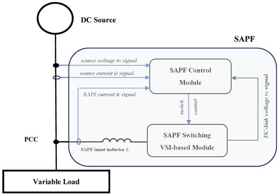
Figure 1. Source-line-load circuitry with SAPF block diagram. PCC is the point of common coupling.

2.2. Reference Signal for SAPF Action

In the DC system, the signal $g_D$, representing the equivalent conductance of the load, can be derived from the instantaneous voltage and current of the load. According to the Fryze–Buchholz–Depenbrock theory [21], this signal is defined as:

$$g_D={\displaystyle \frac{v_s{i}_L}{v_s^2}}$$

(5)

where v_s is the instantaneous source voltage and i_s is instantaneous load current.

The numerator in Equation (5) corresponds to the instantaneous power of the load, while the denominator can be interpreted as the instantaneous squared norm of the source voltage. Accurate acquisition of voltage and current signals is essential for computing the conductance $g_D$.

Based on Equation (5), Depenbrock introduced the so-called power current:

$$i_p=g_D{v}_s$$

(6)

The power current (6) carries only the active power of the load, i.e., it does not deliver the energy related to the energy losses in the SAPF circuitry. However, this loss must not be neglected in practical implementations, and an auxiliary power measurement circuit is commonly employed. Finally, the combined active power of the load and SAPF loads the source. After such complementation of the conductance signal, the reference for the source current can be defined as:

$$i_s^{\ast }\left(t\right)=[g_L\left(t\right)+g_{AF}\left(t\right)]v_s(t)$$

(7)

where $i_s^{\ast }$ denotes the source current reference signal, $g_L$ is the load conductance, and $g_{AF}$ accounts for the losses in the SAPF.

If the source current is controlled in a closed loop according to Equation (7), the compensating current generated by the SAPF does not require explicit computation. Instead, the SAPF inherently produces this current, which can be explained via Kirchhoff’s Current Law. This current corresponds to known as Depenbrock’s “powerless current”, defined as:

$$i_n=i_s-i_p$$

(8)

This component does not contribute to the active power drawn from the source.

3. Reference Signal for the SAPF Action

3.1. Basic Formula Based on Energy Flow Balance

To determine the reference current signal as described in Equation (7)—which comprises the equivalent conductance of both the load and the active filter—an energy-based analysis of the source–active filter–load system was conducted. The following assumptions were adopted regarding the operation of the system:

(1)

Any variation in the load active power P_L, and/or the power losses P_AF in the SAPF, results in a corresponding change in the equivalent conductance signal value.

(2)

Following any such variation, the conductance signal transitions exponentially towards its new steady-state value, characterized by a user-defined time constant τ.

To derive the complete equivalent conductance signal—i.e., a signal representative of both P_L and P_AF—a step change in load power from zero to P_L at time t = 0 can be considered. Assume that the active filter is already operational when the load draws power P_L at t = 0. In accordance with Fryze’s approach [20,21], the total equivalent conductance associated with the load and the active filter can be defined as:

$$G={\displaystyle \frac{P_L+P_{AF}}{V_S^2}}$$

(9)

where $V_S^2$ is the equivalent voltage of the source.

According to the assumptions (1) and (2) the equivalent conductance signal takes the general form for a step change in load power from zero to P_L:

$$g(t)=G\left(1-e^{{\displaystyle \frac{-t}{\tau }}}\right)$$

(10)

Based on the assumptions (1) and (2), the fundamental equation governing the total energy balance (i.e., between the load, active filter, and source) can be expressed as:

$$\left(P_L+P_{AF}\right)t=[W_{AFini}-w_{AF}\left(t\right)]+{\int }_0^t{v}_S{i}_{S}d\varsigma$$

(11)

where: W_AFini is the initial amount of energy stored in the SAPF’s reactive components during the initialization phase; w_AF(t) represents the amount of energy stored at any given time t.

Equation (11) describes that changes in the active power of the load and energy losses in the SAPF cause a transient. During this transient, the energy variations are simultaneously balanced by two distinct energy flows: one delivered by the SAPF’s DC-link capacitor and the other by the supply source. It can be assumed that immediately after the load power changes, the demand is balanced by the active filter solely. Over time, the SAPF’s contribution decreases until a steady state is reached after about four-to-five time constants τ. At this point, the load is already fully supplied by the source.

To describe the energy relation between the source and the SAPF, a parameter N_SF (Source-to-Filter energy ratio) may be defined as:

$$N_{SF}(t)={\displaystyle \frac{W_S[0,t]}{\Delta W_{AF}[0,t]}}={\displaystyle \frac{{\int }_0^t{v}_S{i}_{S}d\varsigma }{W_{AFini}-w_{AF}(t)}}$$

(12)

With the introduction of the NSF parameter, Equation (11) can be reformulated as a function of the SAPF’s energy change alone:

$$(P_L+P_{AF})t=\Delta W_{AF}+W_S=\Delta W_{AF}+\Delta W_{AF}{N}_{SF}(t)=\Delta W_{AF}\left(N_{SF}(t)+1\right)$$

(13)

The overall equation for the equivalent conductance signal can be formulated by dividing (13) by the term $t{V}_S^2$:

$$g(t)={\displaystyle \frac{\left(W_{AFini}-w_{AF}(t)\right)\left(N_{SF}(t)+1\right)}{t{V}_S^2}}$$

(14)

Equation (14) represents the equivalent conductance signal based on the energy stored in the SAPF. This formulation has two key aspects: firstly, the energy flow between the supply source and the load is directly related to the energy stored in the active filter, which corresponds to an indirect control technique; secondly, this approach makes no assumptions regarding the specific system structure, i.e., VSI or CSI converters, in which the active filter operates.

3.2. Energy Flow Balancing in the Source-Active Filter-Load System

To ensure clarity of the discussion, the energy flow in a circuit incorporating an active filter can be analyzed from two perspectives: buffering of load active power variations and management of power generated within the load. It should be noted that these two phenomena may interact to some extent.

(1)

Due to the “implemented inertia” in the operation of the active filter, any change in the load active power is perceived by the source with a certain delay. By appropriately selecting the time constant τ, it is possible to control the level of this inertia, which is directly related to the distribution of energy drawn from the source and from the active filter. The longer the time constant τ, and, therefore, the time required to reach a steady state in the circuit, the greater the level of energy flow buffering by SAPF reactance elements: the DC-link capacitor C and the input smoothing inductor L, as shown later in Equations (15)–(17), Figure 1, and the related commentary. This effect is crucial. It may constitute a beneficial feature of the proposed method: energy flow buffering enables the averaging of the power drawn from the source, thereby reducing source degradation and energy losses in the supply line under variable load conditions.

(2)

The conductance defined by Equation (14) may assume negative values if the instantaneous energy w_AF(t), stored in the active filter, exceeds the initial energy W_AFini, accumulated during the SAPF’s startup phase. Such a situation may occur when the load becomes generative, i.e., it delivers power back to the system. In general, the sign transitions of the conductance—from positive to negative and vice versa—are indicative of energy consumption or generation by the devices interfaced with the active filter. This behavior is independent of whether these devices are connected on the source-load line side or the DC-link side of the SAPF. The exchange of energy among these components can be averaged or buffered by appropriately selecting the value of the parameter τ, which governs the system’s dynamic response.

3.3. Implementation Formula of the Conductance Signal for a VSI-Based SAPF

The active filter can be implemented using a voltage-source inverter (VSI). In such configurations, the SAPF’s energy is primarily stored in the DC-link capacitor and, to a lesser extent, in the SAPF smoothing inductor L. Accordingly, Equation (14) can be reformulated to explicitly represent the energy stored in these reactive components:

$$g(t)=K_V\left(V_{DC-linki\_ini}^2-v_{DC-link}^2(t)\right)+K_I\left(I_{AFini}^2-i_{AF}^2(t)\right)$$

(15)

where the coefficients K_V and K_I are defined as:

$$K_V={\displaystyle \frac{C}{2t{V}_S^2}}$$

(16)

$$K_I={\displaystyle \frac{L}{2t{V}_S^2}}$$

(17)

and where: I_AFini and i_AF(t) denote the SAPF current at the moment the load is switched on and at time t, respectively; C is the capacitance of the DC-link capacitor; L is the inductance of the smoothing inductor L.

The coefficients K_V and K_I quantify the relationship between the energy stored in the reactive components C and L of the SAPF and the resulting conductance signal (15). Specifically, both products on the right-hand side of Equation (15) simplify to the unit expression joule/(second·volt²), which corresponds to siemens. To determine the numerical values of these coefficients, a certain characteristic time t should be assumed. It is convenient to assume t = $\tau$, which facilitates the interpretation of the planned dynamic characteristics of the system. Once these numerical values are adopted, these coefficients can be utilized as proportional gains in P-type controllers, which constitute part of the signal processing unit within the control architecture of the active filter.

Given the implementation formula for the conductance signal $g$, as defined by Equation (15), the reference value of the desired source current can be determined in accordance with the general relationship expressed in Equation (7). This reference takes the form:

$$i_S^{\ast }=g{v}_S$$

(18)

4. Verification of the SAPF Control Method Using Conductance Signal

In modern power electronic systems, DC circuits are increasingly used to supply loads controlled by switching devices such as transistors in converters, motor drives, and pulsed power applications. Although the supply voltage is nominally constant, the presence of switching elements introduces dynamic behavior in the current—and sometimes in the voltage across the load—resulting in time-varying, pulse-shaped waveforms. Traditional methods of power-quality assessment, developed primarily for AC systems, are often inadequate or overly complex when applied to DC environments with switching components. In such cases, some statistical parameters offer a practical alternative for evaluating signal quality and detecting disturbances. Key statistical metrics include: Root Mean Square (rms) Value:—a measure of the energy content of the signal, sensitive to both steady and fluctuating components. Comparing RMS with the average value can reveal the presence of ripple or noise; Standard Deviation (std-dev)—indicates the variability of the signal around its mean, serving as a proxy for signal stability and the effectiveness of filtering mechanisms. This paper explores these two metrics to assess power quality in DC circuits with switching devices.

Basic SAPF Properties

Figure 2 and Figure 3 verify the conductance signal formula (15), showing its response to a step load change for two time constants τ. The SAPF parameters are as follows: DC-link capacitor C = 50 mF, its initial voltage V_DC-link__ini = 500 V, smoothing inductance L = 2 mH. Source voltage Vs = 100 V and its internal resistance R_S = 20 mΩ. The load is a pure resistance R_load = 2 Ω. The time constants τ, see (16) and (17), were assumed to be 50 ms and then 150 ms. Note, the corresponding source current waveforms, given by (18), are proportional to the conductance signals 2 and 3.

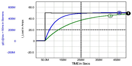
Figure 2. Load current: waveform 1 and conductance signal $g$ at τ (tau in Figure 2) equal to 50 ms and 150 ms: waveforms 2 and 3, respectively. The same Y scale for waveforms 2 and 3.

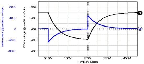
Figure 3. DC-link capacitor voltage: 1. and active filter current: 2. Time constant τ fixed to 50 ms.

The waveforms 2 and 3 shown in Figure 2 confirm that the conductance signal reaches level of 63% of its maximal value after the given time constants τ, equal to 50 ms and 150 ms, respectively. A key feature of this method is the conductance signal’s robustness to changes in system parameters, particularly the gradual decrease in DC-link capacitor capacitance over time. This reduction formally results in an incorrect, excessively high Kv value (Equation (18)) relative to the actual capacitance. However, it only slightly accelerates the system’s transition to steady state.

After a step load switch-on and reaching steady state (Figure 2), the conductance signal (15) and current reference (18) remain constant as long as source voltage and load current are stable. Any change in source voltage or load current (i.e., load power) triggers a transient state in the source–SAPF–load system. During this, conductance g evolves exponentially toward a new value reflecting the updated power flow. The system then settles into a new steady state. The transient duration is user-controlled via the time constant τ, as defined in Equations (15)–(17).

Figure 3 illustrates this feature of the SAPF. This figure shows power/energy processes in the source-SAPF-load system during the turn-on period of 50 ms to 250 ms, and then the turn-off period of 250 ms to 500 ms, for a stationary resistive load of 5 kW. After the load is switched on at t = 50 ms, the system enters a transient state. During this phase, the load draws power, in this case of 5 kW, from both the source and the SAPF in varying proportions. Initially, all the power drawn comes from the SAPF’s DC-link capacitor. This can be confirmed by observing the SAPF current stepping from zero to the magnitude of the full active power of the load, and then its decrease to zero. Energy drawn from the SAPF is confirmed by a drop in DC-link voltage from 500 V to ~490 V. At this level, the system reaches steady state, with all power supplied by the source. The transient lasts approximately 4τ; here, τ = 50 ms. During the transient period, from 50 ms to 250 ms, the load drew energy W_Load = 1000 J. At the same time, the energy output from the DC-link capacitor was 248 J. Considering Equation (19), one can calculate the value of the conductance signal at the end of the transient state: $g(t=250 \mathrm{m}\mathrm{s}$) = 495 mS. The reciprocal of this value is close to 2 Ω, which, according to Fryze’s power theory, is the equivalent load resistance. Applying this value to the source loading with a current appropriate to deliver the required power of 5 kW, see Equation (18), gives a value of 49.5 A, which is sufficiently close to the required value. More accurate calculations, taking into account power losses in the internal resistance of the source and in the active filter, which are not presented here, would require considering energy losses of approximately 100 J.

At t = 250 ms, the load is turned off (Figure 3). The system enters a new transient state, the initial condition of which is that the load is supplied only by the source power, i.e., without the participation of the DC-link capacitor energy. Due to the system inertia defined by the time constant τ, the source cannot immediately stop generating power. Consequently, all the excess source power is captured by the DC-link capacitor. This causes its voltage to increase to a value corresponding to the final source power: in this case, to the initial voltage of 500 V, which corresponds to zero source power. After approximately 4 τ, i.e., about t = 450 ms, the system enters the new steady state with zero power flow.

Figure 4 compares the load current and source current when transmitting energy from the source to the load using PWM control, while Figure 5 shows such currents for a combination of constant load and PWM a controlled load.

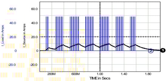
Figure 4. PWM-controlled load. Source current: 1. and load current: 2. Time constant τ is 50 ms.

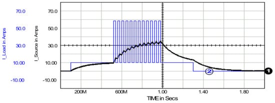
Figure 5. PWM-controlled load with a DC component. Source current: 1. and load current: 2. Time constant τ was set to 50 ms.

The following parameters of the currents shown were obtained: source current rms 6.3 A and standard deviation 2.8 A; and load current rms and std-dev 16.5 A and 15.5 A, respectively. The experiment was conducted with a time constant τ equal to 50 ms. These data confirm the reduction in the source loading due to the SAPF action: reducing the non-active component of the load current, see (8).

Figure 5 shows source and load currents for a combination of constant load and PWM-controlled load, waveforms 1 and 2, respectively. The following parameters of the currents shown were obtained: source current for the time period 100 ms–1.8 s: 17.7 A rms and 10.9 A std-dev; and load current for the time period 100 ms–1.3 s: rms and std-dev 27.6 A and 19.54 A, respectively. The time constant τ was set to 50 ms. Similar to the case shown in Figure 4, these data confirm the reduction of the source loading due to the SAPF compensation for the non-active component of the load current, see (8).

5. Tuning of the SAPF Functionality

The SAPF control method considered in this article, using a conductance signal, offers unique opportunities for tuning its operation to achieve the desired results. In particular, it is possible to reduce the unwanted component in the source current not only by selecting an appropriate time constant τ, but also by imposing certain constraints on the conductance signal’s range of variation. These opportunities are presented in this section. They are presented in the context of a certain reference load current, described below.

5.1. Considered Load Current

To compare various possibilities for achieving the desired source current or power quality, a reference load current waveform was adopted. It was chosen arbitrarily, but such that it would be “difficult” to compensate. Specifically, this waveform contains a constant load component and a PWM-controlled load component. An active component was also considered, where a load component within the SAPF compensation loop switches to generator mode. This reference waveform is shown in Figure 6.

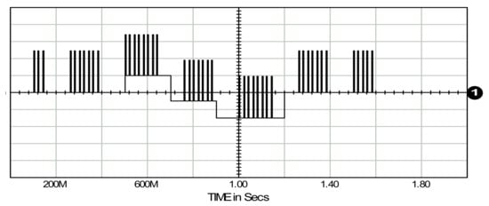
Figure 6. Considered load current. Considered load current waveform.

The load current waveform includes certain characteristic periods associated with different types of compensated load operation. The waveform includes seven pulsed (PWM) load “segments”. The first segment is active in the time interval of 100 ms–150 ms, the last one from 1.5 s to 1.6 s. At time t = 500 ms, a 2 kW load (current 20 A at a source voltage of 100 V) is activated. It is turned off at time t = 900 ms. Then, at time t = 700 ms, the generating element is turned on, operating until to 1.2 s at a power of 3 kW (current of 30 A at voltage of 100 V).

The load current parameters used to assess the effectiveness of compensation for the reference current were the effective rms value and the standard deviation std-dev, which in the time interval of 0.1 s to 1.6 s were 23.5 A rms and 23.3 A std-dev.

5.2. Selection of the Time Constant

A natural method to reduce the rms and standard deviation of the source current relative to the load current is to appropriately select the time constant τ, see Figure 2. Increasing this constant leads to an increased averaging contribution of the SAPF to the energy flow between the source and the load. Figure 7 shows the effect that can be achieved in this way. It shows the source current waveforms 1 and 2 for time constants set to 50 ms and 200 ms, respectively.

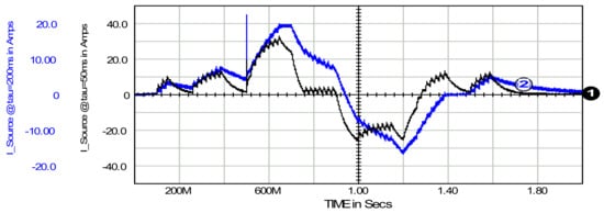
Figure 7. Source current at τ = 50 ms, waveform 1, and τ = 200 ms, waveform 2, respectively.

Changing the time constant from a magnitude of 50 ms to 200 ms causes the rms to decrease from 13.8 A to 8.7 A and the std-dev to decrease from 13.5 A to 8.4 A, respectively. Reducing these source current parameters comes at the cost of widening the DC-link capacitor voltage range of voltage and increasing its peak-to-peak voltage variation. This phenomenon is shown in Figure 8.

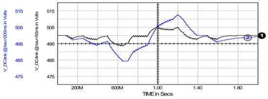
Figure 8. DC-link capacitor voltage at τ = 50 ms, waveform 1; and τ = 200 ms, waveform 2, respectively.

Extending the DC-link capacitor voltage range slightly modifies the SAPF’s operating dynamics, increasing them at higher voltages and decreasing them at lower voltages. For a properly selected DC-link capacitor, its initial voltage, and the range of power changes of the compensated load, this effect is marginal and can be neglected.

5.3. Limitation of the Conductance Signal Variation Range

The SAPF control method under consideration allows unique control of power flow in the system by imposing limits on the maximum and minimum values of the conductance signal. The achieved effects are similar to the previously described increase in the time constant τ. Figure 9 shows the source current waveform with an unlimited and then a limited range of conductance signal variation. Note that for a known source voltage of 100 V, the conductance signal waveform can be unambiguously obtained based on the source current waveform, see (18).

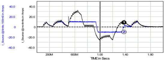
Figure 9. Source current at τ = 50 ms and no limits on conductance signal, waveform 1; and source current at τ = 50 ms and conductance signal limited to range of ±100 mS, waveform 2.

Limiting the conductance signal to the range ±100 mS causes the source current rms to decrease from 13.7 A to 8.3 A and the std-dev to decrease from 13.5 A to 7.9 A, respectively. Similarly to the increase in the time constant, the reduction in rms and std-dev parameters is achieved at the expense of widening the range of voltage variations. This phenomenon is shown in Figure 10.

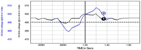
Figure 10. DC-link capacitor voltage with no constraints on the conductance signal, waveform 1; and with ±100 mS constraints, waveform 2, respectively. Time constant τ was set to 50 ms.

Table 1 summarizes the effects of the various methods discussed above for reducing the RMS and standard deviation parameters of the source current relative to the reference load current.

Table 1. Summary of SAPF simulation result, related to Figure 6, Figure 7 and Figure 9.

Circuit Description	Section/ Figure	RMS [A]	Std-Dev [A]	RMS Reduction vs. Reference [%]	Std-Dev Reduction vs. Reference [%]
Load reference current	5.1/6	23.5	23.3	-	-
Source current at τ = 50 ms	5.2/7	13.8	13.5	59	58
Source current at τ = 200 ms	5.2/7	8.7	8.4	37	36
Source current at τ = 50 ms and conductance signal limited to ±100 mS	5.3/9	8.3	7.9	35	34

Limiting the conductance signal range is especially relevant when it becomes negative—e.g., upon activation of a relatively powerful generator among the compensated devices. This scenario was implemented for the reference load current between 700 ms and 1200 ms (see Figure 6 and its description). Figure 11 illustrates the power flow in the source–SAPF–load system, which can be divided into five stages.

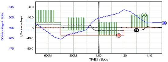
Figure 11. Current generated in the load, waveform 1; total load current, waveform 2; source current, waveform 3; and DC-link capacitor voltage, waveform 4. The scale of all current waveforms is the same, as shown for waveform 3. Time constant τ was set to 50 ms.

In the first stage (500–700 ms), the load is passive. The load current has a pulsed and a constant component. Since the conductance signal is limited to 100 mS, the source current cannot exceed 10 A. This value is too low to deliver the required power to the load from the source. This lack of power is balanced by the DC-link capacitor, whose energy and voltage decrease. During this stage, the energy dissipated in the load is 600 J. At the same time, the energy drawn from the source is 200 J, and the energy drawn from the DC-link capacitor is 400 J.

The second stage (700–900 ms) begins with switching on a 3 kW generator in the load branch at t = 700 ms (see waveform 1). Since the generator power exceeds the 2 kW load, the surplus cannot flow back to the source due to the positive conductance signal (see (15) and (18)). Consequently, the load current reverses direction, while the source current does not. The excess power charges the DC-link capacitor, increasing its voltage. The temporary PWM load (760–890 ms) and the disconnection of the 2 kW DC load at t = 900 ms do not affect the overall power flow.

The third stage (0.9–1.0 s) is important for describing the system operation. As a result of the continuous accumulation of energy, the DC-link capacitor voltage approaches its initial magnitude, set here at 500 V, and the conductance signal enters the active region within a range of ±100 mS, enabling control of the source current. This occurs between (930–970 ms): the DC-link capacitor voltage increases from 498 V to 502 V, and the source current is then overdriven from 10 A to −10 A. This change in both sign and value of the source current results from the change in the conductance signal from 100 mS to −100 mS; see (15) and (18). During this time interval, the power dissipated in the load is zero, so the power generated in the load is, in varying proportions, partly transmitted to the source and partly stored in the DC-link capacitor.

The fourth stage (1.0–1.2 s) shows the process of dividing the power generated in the load into power accumulated in the DC-link capacitor and power transmitted with the allowed amount upstream to the source.

The fifth stage (1.2–1.4 s) begins with the moment of power generation switch-off in the compensated load. The energy stored in the DC-link capacitor is primarily transmitted to the source with a power adequate to the −100 mS conductance signal limit, and in the remaining part, it powers the PWM load. At the very end of this stage, the energy accumulated in the DC-link capacitor is depleted, and the source takes over the power supply to the load for a short while.

6. Power/Load Connection to the DC-Link Capacitor Terminals

The conductance signal is obtained in the SAPF Control Module by tracking the energy stored in the DC-link capacitor and the input inductor L; see Figure 1. The data presented in Section 4 and Section 5, including the analysis of powers and currents, indicate that the amount of energy stored in the inductor L is small compared to the energy stored in the DC-link capacitor. Therefore, its influence on the calculation of the conductance signal can be neglected. This observation leads to the possibility of omitting the second, “current”, term of the sum in Equation (15).

In the cases discussed so far, the DC-link capacitor energy was changed only using a converter; see SAPF Switching VSI-based Module in Figure 1. However, there is the obvious option of connecting a load or generator to the DC-link capacitor terminals. This would allow bidirectional energy exchange with the lower voltage side loads and the source through this additional port. In particular, it enables energy to be stored or discharged in the DC-link capacitor independently of the lower voltage side circuit. Both the absorption and delivery of energy to the DC-link capacitor, whether via a SAPF converter or directly to the capacitor terminals, change the voltage on it. As a result, the conductance signal also changes. As shown in Section 5, system behavior can be controlled by setting the time constant τ and/or by adopting a convenient limit for the conductance signal variation range. This allows for three scenarios: (a) returning the energy to the higher voltage side circuit, (b) directing the energy to the lower voltage side circuit with the possibility of transferring it upstream to the source, or blocking such transfer. In the latter case, the energy stored in the DC-link capacitor can be intended for use by loads or the source on the lower voltage side of the system. The implementation of energy storage directly in the DC-link capacitor and its consumption in the load on the lower voltage side, without upstream transmission towards the source, is shown in Figure 12 and Figure 13. A simple scenario is used, but it demonstrates the point clearly.

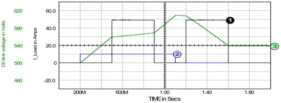
Figure 12. Load current, waveform 1; DC-link capacitor charging current, waveform 2, and DC-link capacitor voltage, waveform 3. The Y-axis scales for both current waveforms are the same.

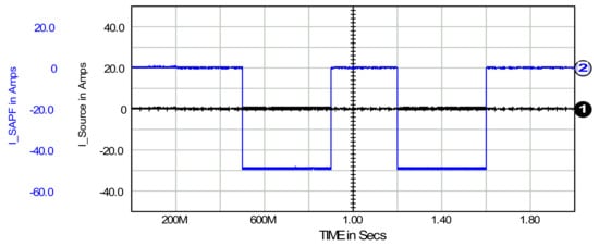
Figure 13. Source current, waveform 1, and SAPF current, waveform 2.

In the time period from 200 ms to 1.1 s, the DC-link capacitor is supplied from the higher voltage side with a power of 5.9 kW; Figure 12. On the lower voltage side, a 5 kW load is switched on twice: in the period from 600 ms to 900 ms and then from 1.2 s to 1.6 s. As a result, the total energy drawn by this load is 3888 J. During the entire period of the DC-link capacitor’s active operation, i.e., from 200 ms to 1.6 s, its energy balance is: 5320 J delivered minus 3888 J drawn, resulting in a surplus of 1432 J over the initial level. This energy surplus is seen as a 40 V increase over the initial magnitude of 500 V in the capacitor voltage at time t > 1.6 s, along with 392 J of energy dissipated in the SAPF converter.

Figure 13 shows the SAPF current and the source current. The SAPF current here is not a compensating current in the usual sense. If the classical compensation method were applied, the SAPF current would be the non-active component of the load current. However, in the present case, its average value, i.e., the DC component, is equal to the active current of the load, thereby delivering the entire active power to the load. This active power is drawn from the DC-link capacitor, which is supplied from the higher voltage side–time interval 200 ms–1100 ms, waveform 2. Consequently, the source current on the lower voltage side is zero (neglecting the pulse current resulting from the hysteresis control of the VSI converter switches within the SAPF).

Operating the SAPF with a zero-source current is a special case, intended here to demonstrate a non-standard application of the SAPF within the discussed method of controlling the SAPF based on a conductance signal.

7. Conclusions

This paper has presented and verified an advanced control method for Shunt Active Power Filters (SAPFs) specifically tailored for improving power quality and managing energy flow in DC-powered systems, with a particular focus on systems integrating electrochemical energy sources such as batteries and fuel cells.

The core contribution of this work is the implementation of a SAPF control strategy based on a dynamically calculated equivalent conductance signal. This approach offers significant advantages:

• Sensorless Control: By deriving the conductance signal primarily from the DC-link capacitor voltage, the method eliminates the necessity for additional current or power sensors, leading to a simplified and more efficient control design.
• Effective Non-Active Current Compensation: The SAPF demonstrably reduces non-active current components, leading to a substantial decrease in the root mean square (RMS) and standard deviation (std-dev) of the source current, thus improving overall power quality.
• Enhanced Source Protection: By averaging the power drawn from the source and stabilizing current changes, the method significantly mitigates the detrimental effects of rapid load variations on batteries and fuel cells, thereby extending their operational lifespan and improving reliability.
• Flexible Power Management: The ability to tune the system’s dynamic response through a user-defined time constant (τ) and to impose limits on the conductance signal’s variation range provides unprecedented control over energy flow buffering and management of generative loads. This includes the unique capability to redirect generated power to local loads or store it in the DC-link capacitor without returning it to the main source.
• Universal Applicability: The underlying energy-based formulation of the conductance signal ensures its applicability across various DC and AC system configurations, including those employing different inverter types.

The simulation verification, supported by numerous waveform analyses, confirms the robust and effective performance of the proposed SAPF control method across diverse operating conditions. This research underscores the potential of advanced SAPF control using the equivalent conductance signal to significantly improve the stability, efficiency, and longevity of modern DC-powered systems, especially in applications with sensitive electrochemical energy storage and dynamic loads.

References

- Barros, J.; Apraiz, M.; Diego, R.I. Definition and measurement of power quality indices in low voltage DC networks. In Proceedings of the IEEE 9th International Workshop on Applied Measurements for Power Systems (AMPS), Bologna, Italy, 26–28 September 2018. [Google Scholar]
- Barros, J.; Apraiz, M.; Diego, R.I. Power Quality in DC Distribution Networks. Energies 2019, 12, 848. [Google Scholar] [CrossRef]
- Liao, J.; Liu, Y.; Guo, C.; Zhou, N.; Wang, Q.; Kang, W.; Vasquez, J.C.; Guerrero, J.M. Power quality of DC microgrid: Index classification, definition, correlation analysis and cases study. Int. J. Electr. Power Energy Syst. 2024, 156, 109782. [Google Scholar] [CrossRef]
- Bahloul, M.; Khadem, S. Impact of Power Sharing Method on Battery Life Extension in HESS for Grid Ancillary Services. IEEE Trans. Energy Convers. 2019, 34, 1317–1327. [Google Scholar] [CrossRef]
- Carter, R.; Cruden, A.; Hall, P.J. Optimizing for Efficiency or Battery Life in a Battery/Supercapacitor Electric Vehicle. IEEE Trans. Veh. Technol. 2012, 61, 1526–1533. [Google Scholar] [CrossRef]
- Timilsina, L.; Badr, P.R.; Hoang, P.H.; Ozkan, G.; Papari, B.; Edrington, C.S. Battery Degradation in Electric and Hybrid Electric Vehicles: A Survey Study. IEEE Access 2023, 11, 42431–42462. [Google Scholar] [CrossRef]
- Elmahallawy, M.; Elfouly, T.; Alouani, A.; Massoud, A.M. A Comprehensive Review of Lithium-Ion Batteries Modeling, and State of Health and Remaining Useful Lifetime Prediction. IEEE Access 2022, 10, 119040–119070. [Google Scholar] [CrossRef]
- Menye, J.S.; Camara, M.-B.; Dakyo, B. Lithium Battery Degradation and Failure Mechanisms: A State-of-the-Art Review. Energies 2025, 18, 342. [Google Scholar] [CrossRef]
- Rahman, T.; Alharbi, T. Exploring Lithium-Ion Battery Degradation: A Concise Review of Critical Factors, Impacts, Data-Driven Degradation Estimation Techniques, and Sustainable Directions for Energy Storage Systems. Batteries 2024, 10, 220. [Google Scholar]
- Lipu, M.S.H.; Al Mamun, A.; Ansari, S.; Miah, M.S.; Hasan, K.; Meraj, S.T.; Abdolrasol, M.G.M.; Rahman, T.; Maruf, M.H.; Sarker, M.R.; et al. Battery Management, Key Technologies, Methods, Issues, and Future Trends of Electric Vehicles: A Pathway toward Achieving Sustainable Development Goals. Batteries 2022, 8, 119. [Google Scholar] [CrossRef]
- Jin, S.; Huang, X.; Sui, X.; Wang, S.; Teodorescu, R.; Stroe, D.-I. Overview of Methods for Battery Lifetime Extension. In Proceedings of the EPE’21 ECCE Europe, Ghent, Belgium, 6–10 September 2021. [Google Scholar]
- Cai, F.; Cai, S.; Tu, Z. Proton exchange membrane fuel cell (PEMFC) operation in high current density (HCD): Problem, progress and perspective. Energy Convers. Manag. 2024, 307, 118348. [Google Scholar] [CrossRef]
- Shi, Y.; Janssen, H.; Lehnert, W.A. Transient Behavior Study of Polymer Electrolyte Fuel Cells with Cyclic Current Profiles. Energies 2019, 12, 2370. [Google Scholar] [CrossRef]
- Wu, Q.; Li, S.; Hou, Z.; Lu, L.; Gu, X.; Chen, H.; Luan, W. Review of control strategies for onboard fuel cells: Insights from degradation mechanisms under variable load conditions. Int. J. Hydrogen Energy 2024, 110, 628–645. [Google Scholar] [CrossRef]
- Saidouini, W.H.; Marchand, M.; Gerard, D.; Jemei, S.; Bouquain, D. Impact of start-stop and load cycling on the lifetime of PEMFC-powered vehicles. In Proceedings of the IEEE Vehicle Power and Propulsion Conference (VPPC), 2024, Washington, DC, USA, 7–10 October 2024. [Google Scholar]
- Luca, R.; Whiteley, M.; Neville, T.; Shearing, P.; Brett, D.J.L. Comparative study of energy management systems for a hybrid fuel cell electric vehicle—A novel mutative fuzzy logic controller to prolong fuel cell lifetime. Int. J. Hydrogen Energy 2022, 47, 24042–24058. [Google Scholar] [CrossRef]
- Zhao, X.; Wang, L.; Zhou, Y.; Pan, B.; Wang, R.; Wang, L.; Yan, X. Energy management strategies for fuel cell hybrid electric vehicles: Classification, comparison, and outlook. Energy Convers. Manag. 2022, 270, 116179. [Google Scholar] [CrossRef]
- Ahmadi, S.; Bathaee, S.M.T.; Hosseinpour, A.H. Improving fuel economy and performance of a fuel-cell hybrid electric vehicle (fuel-cell, battery, and ultra-capacitor) using optimized energy management strategy. Energy Convers. Manag. 2018, 160, 74–84. [Google Scholar] [CrossRef]
- Marzougui, H.; Amari, M.; Kadri, A.; Bacha, F.; Ghouili, J. Energy management of fuel cell/battery/ultracapacitor in electrical hybrid vehicle. Int. J. Hydrogen Energy 2017, 42, 8857–8869. [Google Scholar] [CrossRef]
- Fryze, S. Wirk-, Blind-, und Scheinleistung in Elektrischen Stromkreisen mit nichtsinusformigem Verlauf von Strom und Spannung. Elektrotech. Z. 1932, 25, 33. [Google Scholar]
- Depenbrock, M.; Staudt, V. The FBD-method as tool for compensating non-active currents. In Proceedings of the 8th International Conference on Harmonics and Quality of Power, Athens, Greece, 14–16 October 1998; pp. 320–324. [Google Scholar]
- Asiminoaei, L.; Blaabjerg, F.; Hansen, S. Detection is key. Harmonic detection methods for active power filter applications. IEEE Ind. Appl. Mag. 2007, 13, 22–33. [Google Scholar] [CrossRef]
- Boopathi, R.; Indragandhi, V. Comparative analysis of control techniques using a PV-based SAPF integrated grid system to enhance power quality. Adv. Electr. Eng. Electron. Energy 2023, 5, 100222. [Google Scholar] [CrossRef]
- Babu, N. Adaptive grid-connected inverter control schemes for power quality enrichment in microgrid systems: Past, present, and future perspectives. Electr. Power Syst. Res. 2024, 230, 110288. [Google Scholar] [CrossRef]
- Duc, M.L.; Hlavaty, L.; Bilik, P.; Martinek, R. Harmonic Mitigation Using Meta-Heuristic Optimization for Shunt Active Power Filters: A Review. Energies 2023, 16, 3998. [Google Scholar] [CrossRef]
- Hoon, Y.; Radzi, M.A.M.; Hassan, M.K.; Mailah, N.F. Control Algorithms of Shunt Active Power Filter for Harmonics Mitigation: A Review. Energies 2017, 10, 2038. [Google Scholar] [CrossRef]
- Moreno, V.; Pigazo, A. Modified FBD method in active power filters to minimize the line current harmonics. IEEE Trans. Power Del. 2006, 22, 735–736. [Google Scholar] [CrossRef]
- Strzelecki, R.; Benysek, G.; Jarnut, M. Power quality conditioners with minimum number of current sensor requirement. Przegląd Elektrotech. (Electrotech. Rev.) 2008, 84, 295–298. [Google Scholar]
- Sharma, S.; Verma, V. Modified control strategy for shunt active power filter with MRAS-based DC voltage estimation and load current sensor reduction. IEEE Trans. Ind. Appl. 2021, 57, 1652–1663. [Google Scholar] [CrossRef]
- Szromba, A.; Mysinski, W. Voltage-source-based conductance-signal controlled shunt active power filter. In Proceedings of the 2017 European Conference on Power Electronics and Applications, Warsaw, Poland, 11–14 September 2017. [Google Scholar]
- Szromba, A. The Unified Power Quality Conditioner Control Method Based on the Equivalent Conductance Signals of the Compensated Load. Energies 2020, 13, 6298. [Google Scholar] [CrossRef]
- Nunez-Zuninga, T.; Pomilio, J. Shunt active power filter synthesizing resistive loads. IEEE Trans. Power Electron. 2002, 17, 273–278. [Google Scholar] [CrossRef]
- Fukuda, S.; Kanayama, T.; Muraoka, K. A current control method for active filters without detecting current harmonics. In Proceedings of the Fifth International Conference on Power Electronics and Drive Systems, 2003, PEDS 2003, Singapore, 17–20 November 2003; Volume 1, pp. 519–524. [Google Scholar]
- Ozdemir, E.; Ucar, M.; Kesler, M.; Kale, M. A simplified control algorithm for shunt active power filter without load and filter current measurement. In Proceedings of the IECON 2006-32nd Annual Conference on IEEE Industrial Electronics, Paris, France, 7–10 November 2006; pp. 2599–2604. [Google Scholar]
- Nedeljkovic, D.; Nemec, M.; Drobnic, K.; Ambrozic, V. Direct current control of active power filter without filter current measurement. In Proceedings of the 2008 International Symposium on Power Electronics, Electrical Drives, Automation and Motion, Ischia, Italy, 11–13 June 2008; pp. 72–76. [Google Scholar]
- Ketzer, M.B.; Jacobina, C.B. Multivariable load current sensorless controller for universal active power filter. IET Power Electron. 2014, 7, 1777–1786. [Google Scholar] [CrossRef]
Disclaimer/Publisher’s Note: The statements, opinions and data contained in all publications are solely those of the individual author(s) and contributor(s) and not of MDPI and/or the editor(s). MDPI and/or the editor(s) disclaim responsibility for any injury to people or property resulting from any ideas, methods, instructions or products referred to in the content. |
© 2025 by the author. Licensee MDPI, Basel, Switzerland. This article is an open access article distributed under the terms and conditions of the Creative Commons Attribution (CC BY) license (https://creativecommons.org/licenses/by/4.0/).