E2E-MDC: End-to-End Multi-Modal Darknet Traffic Classification with Conditional Hierarchical Mechanism

Abstract

Accurate identification and classification of Darknet traffic is a critical technical challenge for network security supervision. Existing methods predominantly adopt single-modal features and independent classification strategies, making it difficult to effectively handle the hierarchical structural characteristics and complex encryption patterns of Darknet traffic. This paper proposes E2E-MDC (End-to-End Multi-modal Darknet Classification), an end-to-end deep learning framework based on conditional hierarchical mechanism for three-level hierarchical classification of Darknet traffic. The framework integrates four complementary feature extractors—byte-level CNN, packet sequence TCN, bidirectional LSTM, and Transformer—to comprehensively capture traffic patterns from multiple perspectives. A soft conditional hierarchical classification architecture explicitly models dependencies among Level 1 (Darknet type), Level 2 (application category), and Level 3 (specific behavior) by using upper-level prediction probability distributions as conditional input for lower-level classification. On the self-collected Tor dataset containing 8 applications and 8 behavior types, the system achieves 94.90% cascade accuracy, with Level 3 fine-grained classification accuracy reaching 95.02%. On the public Darknet-2020 dataset, cascade accuracy reaches 92.65%, representing improvements of 12% and 15% over existing state-of-the-art methods, respectively, while reducing hierarchical violation rate to below 0.8%. Experimental results demonstrate that the conditional hierarchical mechanism and multi-modal fusion strategy significantly enhance the accuracy and robustness of Darknet traffic classification, providing effective technical support for network security protection.

1. Introduction

With the rapid development of Internet technology, the Darknet has increasingly attracted widespread attention as a special network space. The Darknet refers to network spaces built upon Internet infrastructure that require specific software, configurations, or authorization to access. It primarily includes anonymous communication systems such as Tor (The Onion Router), I2P (Invisible Internet Project), Freenet, and ZeroNet. Although the original intention of Darknet technology is to protect user privacy and freedom of speech, its strong anonymity and encryption characteristics are also exploited for malicious purposes [1], making it a breeding ground for cybercrime, illegal transactions, terrorism, and other activities. Therefore, accurate identification and classification of Darknet traffic is of great significance for network security supervision, crime prevention, and forensic investigation.

Darknet traffic classification faces multiple technical challenges. First, Darknet protocols employ multi-layer encryption and onion routing technologies, rendering traditional Deep Packet Inspection (DPI)-based methods [2] ineffective. The encrypted payload prevents direct content inspection, while onion routing obscures the true source and destination of traffic. Second, traffic characteristics differ significantly across different Darknet platforms (Tor, I2P, Freenet, ZeroNet), while traffic patterns of different applications within the same platform are highly similar, creating difficulties for fine-grained classification. Third, the dynamic and adversarial nature of Darknet traffic requires classification methods to possess good robustness and adaptability to handle diverse traffic patterns and evasion techniques. Finally, practical applications need to meet real-time requirements while ensuring classification accuracy, imposing strict constraints on algorithm efficiency.

Existing Darknet traffic classification methods can be mainly divided into two categories. Traditional machine learning methods [3,4,5,6] rely on manually designed statistical features, such as packet size distribution, inter-packet intervals, and flow duration. Although these methods perform well in certain scenarios, they have inherent limitations. Feature engineering is time-consuming and labor-intensive, requiring extensive domain expertise. More critically, handcrafted statistical features struggle to capture deep temporal relationships in encrypted traffic, where the temporal ordering and dependencies of packets often carry crucial discriminative information that simple statistics cannot adequately represent.

In recent years, deep learning methods have begun to be applied in this field, demonstrating the capability for automated feature learning. DarkDetect [7] adopts a CNN-LSTM hybrid architecture, achieving 96% accuracy on darknet detection tasks. DIDarknet [8] converts traffic into images for classification using pre-trained ResNet-50. DarknetSec [9] introduces self-attention mechanisms to explore feature relationships. However, these methods exhibit several limitations that motivate our work.

First, most existing deep learning methods focus only on single-level classification tasks, ignoring the hierarchical structural characteristics of Darknet traffic. In practice, Darknet traffic naturally follows a three-level hierarchy: platform type (e.g., Tor, I2P), application category (e.g., Telegram, BBC), and specific behavior (e.g., video, browsing). Methods that treat classification as a flat problem fail to leverage this structural prior and may produce logically inconsistent predictions. For instance, a classifier might incorrectly predict “Freenet platform” at level 1 while simultaneously predicting “Telegram application” at level 2, violating the inherent constraint that Telegram only operates on Tor.

Second, existing methods mostly adopt single-modal features, failing to fully utilize multi-dimensional information in traffic data. DarkDetect [7] primarily relies on CNN-extracted spatial features and LSTM-captured temporal patterns, but does not consider raw byte-level information. DIDarknet [8] focuses exclusively on image-based representations converted from traffic matrices. DarknetSec [9] emphasizes statistical features with attention mechanisms. Each approach captures only a partial view of the traffic characteristics. Given that encrypted Darknet traffic exhibits complex patterns across multiple dimensions—byte-level protocol signatures, packet-level statistical distributions, flow-level temporal dynamics, and session-level global semantics—a single modality is inherently insufficient for comprehensive characterization.

Third, even among the few works that consider hierarchical classification [10,11], most employ independent classifiers at each level without explicitly modeling inter-level dependencies. This approach treats each level as a separate task, potentially leading to hierarchical violations where predictions at different levels are mutually inconsistent. Such violations not only indicate classification errors but also reduce the interpretability and trustworthiness of the system in security-critical applications.

To address these limitations, this paper proposes E2E-MDC (End-to-End Multi-modal Darknet Classification), an end-to-end deep learning framework based on conditional hierarchical mechanism for three-level hierarchical classification of Darknet traffic. The framework integrates four complementary feature extractors—byte-level CNN, packet sequence TCN, bidirectional LSTM, and Transformer—to comprehensively capture traffic patterns from multiple perspectives. A soft conditional hierarchical classification architecture explicitly models dependencies among Level 1 (Darknet type), Level 2 (application category), and Level 3 (specific behavior) by using upper-level prediction probability distributions as conditional input for lower-level classification.

Experimental results demonstrate that our method achieves a cascade accuracy of 94.90% on the self-collected Tor traffic dataset and 92.65% on the public Darknet-2020 dataset, representing improvements of 12% and 15% over existing state-of-the-art methods, respectively, while reducing the hierarchical violation rate to below 0.8%. Ablation experiments confirm the effectiveness of multi-modal fusion and conditional hierarchical design. Furthermore, the system achieves an inference speed of 1200 traffic windows per second on an RTX 3090 GPU (NVIDIA Corporation, Chengdu, China), meeting real-time detection requirements.

The main contributions of this paper are summarized as follows:

• Innovative proposal of a conditional hierarchical classification mechanism. Unlike traditional independent multi-task learning or hard cascade classification, this paper implements end-to-end hierarchical learning through a soft conditioning design that enables joint optimization across all classification levels. Specifically, the probability distribution (rather than hard decisions) of upper-level classification is used as conditional input for lower levels, enabling gradient backpropagation through Softmax operations while preserving prediction uncertainty information. This design maintains cascade accuracy of 94.90% while controlling the hierarchical violation rate below 0.8%.
• Design of a four-modal complementary feature extraction architecture tailored for Darknet traffic characteristics. Targeting different information dimensions of encrypted traffic, this paper carefully designs four specialized neural network modules: (i) byte-level CNN captures encrypted protocol patterns through learnable byte embeddings; (ii) temporal convolutional network employs exponentially growing dilation rates (1, 2, 4, 8) to extract multi-scale temporal patterns; (iii) bidirectional LSTM fuses recurrent features with self-attention outputs through gating mechanisms; (iv) Transformer employs a [CLS] token mechanism to provide global sequence representation for traffic classification. Experiments demonstrate that this complementary design achieves 95.02% accuracy in Level 3 fine-grained classification.
• Proposal of a multi-objective joint optimization framework that unifies classification accuracy, hierarchical consistency, and feature diversity in an end-to-end differentiable loss function. Through carefully designed loss weights (classification 0.3/0.3/0.4, consistency 0.1, diversity 0.01), the system effectively maintains logical reasonability of predictions while optimizing the main task and prevents model degradation into single-modal dependency.
• Construction of a fine-grained Tor traffic benchmark dataset containing 6240 annotated samples across 8 behavior categories from 8 mainstream applications (BBC, Twitter, Telegram, etc.), employing a sliding window mechanism (window size 2000 packets, step size 1500 packets) to ensure completeness of traffic patterns, providing a new evaluation benchmark for Darknet traffic classification research.

The organization of this paper is as follows: Section 2 introduces related research work; Section 3 provides a formal definition of the problem and elaborates on the proposed end-to-end multi-modal classification system; Section 4 conducts experimental validation and result analysis; Section 5 concludes the paper and outlines future research directions.

2. Background and Related Work

In this section, we introduce the relevant background of the darknet and review related research in the field of machine learning-based darknet traffic classification.

2.1. Darknet

The darknet is a part of the Internet that is hidden from ordinary search engine indexing and requires special software and configuration to access. Mainstream darknet technologies include the following:

Tor network [12] is the most widely used darknet platform. It employs onion routing technology to achieve anonymous communication through three-layer encryption and multi-hop forwarding. Traffic passes through entry nodes, relay nodes, and exit nodes, with each hop only knowing the adjacent nodes before and after, making it impossible to trace the complete path. Tor supports the TCP protocol and is widely used for anonymous browsing, instant messaging, and other applications.

I2P network focuses on hidden services and employs garlic routing technology, which bundles and encrypts multiple messages together. Unlike Tor, all nodes in I2P function as both clients and routers, forming a fully distributed overlay network. I2P has built-in support for various applications, including email, file sharing, and web browsing.

Freenet is a distributed censorship-resistant storage system that uses content-based routing mechanisms. Data is encrypted, fragmented, and redundantly stored across multiple nodes, retrieved through keys. Freenet emphasizes content persistence and censorship resistance, making it suitable for publishing and retrieving static content.

ZeroNet uses Bitcoin cryptography and the BitTorrent network to create decentralized websites. Each website is a torrent file, and visitors simultaneously serve as content distributors. ZeroNet does not provide anonymity by default and typically needs to be used in conjunction with Tor.

The common characteristics of these darknet technologies—strong encryption, multi-layer forwarding, and traffic obfuscation—pose tremendous challenges for traffic classification.

2.2. Traditional Machine Learning-Based Methods

Early darknet traffic classification research primarily employed traditional machine learning methods. The core of these methods lies in feature engineering, i.e., extracting statistical features from raw traffic for classification.

In terms of feature selection, researchers have explored various approaches. Recent feature selection review studies [13] systematically summarize filtering, wrapper, and embedded feature selection paradigms. By combining the advantages of multiple algorithms [14], more stable feature subsets can be obtained. Commonly used features include packet size statistics (mean, variance, maximum, minimum), inter-packet interval time distribution, packet direction ratio, byte distribution entropy, and flow duration.

Regarding classifier selection, Random Forest [3] is widely used due to its robustness to high-dimensional features. Rust-Nguyen et al. [1] achieved 98% accuracy on the CIC-Darknet2020 dataset through optimized Random Forest. Marim et al. [4] compared the performance of decision trees and neural networks in darknet traffic detection. Gradient boosting tree methods have shown excellent performance in recent years. XGBoost [5] and LightGBM [6], as next-generation gradient boosting frameworks, have demonstrated superior performance in darknet traffic classification. Song et al. [15] proposed the CDBC method, improving XGBoost’s effectiveness in darknet detection through enhanced between-class learning. Ensemble learning methods further improve performance by combining multiple base learners. Almomani [16] proposed an improved stacking ensemble framework, achieving 99% accuracy in the training phase. Mohanty et al. [17] designed a robust stacking ensemble model that maintains stable performance in adversarial environments.

However, the main limitations of traditional methods are (1) heavy reliance on hand-crafted features, making it difficult to adapt to dynamic changes in traffic patterns; (2) inability to capture deep patterns in raw traffic; and (3) significant performance degradation on fine-grained classification tasks.

2.3. Deep Learning-Based Methods

Deep learning methods overcome some limitations of traditional methods by automatically learning feature representations. DIDarknet, proposed by Lashkari et al. [8], is a pioneering work in this field, converting traffic data into grayscale images and utilizing pre-trained ResNet-50 for classification, achieving excellent performance on binary classification tasks. The innovation of this image-based method lies in mapping temporal traffic to two-dimensional space, leveraging mature computer vision techniques.

CNN-LSTM hybrid architectures are widely applied to traffic classification. DarkDetect, proposed by Sarwar et al. [7], employs a 3-layer CNN to extract spatial features and a 2-layer LSTM to model temporal dependencies, achieving 96% and 89% accuracy on darknet detection and classification tasks respectively. This architecture combines CNN’s local feature extraction capability with LSTM’s sequence modeling ability. Other innovative deep learning architectures have also been applied to this field. FlowPic [18] provides a general traffic representation learning framework by converting network traffic into image representations. CETAnalytics [19] combines content features and statistical features, using Bi-GRU to process temporal information. DarknetSec [9] introduces self-attention mechanisms, exploring intrinsic relationships between features through multi-head attention.

2.4. Multi-Modal Traffic Classification

Recent advances in deep learning have demonstrated the effectiveness of multi-modal approaches for encrypted traffic classification. These methods leverage complementary information from different data modalities to improve classification performance.

Lin et al. [20] proposed a novel multimodal deep learning framework called PEAN for encrypted traffic classification. Their method combines packet-level and flow-level features through separate neural networks. Aceto et al. [2] developed MIMETIC, a multimodal mobile encrypted traffic classification system. It integrates data payload and protocol time-series features through deep learning models. More recently, Zhai et al. [21] introduced ODTC, an online darknet traffic classification model. It employs CNN and BiGRU to extract spatiotemporal features from payload content. ODTC also uses a multi-head attention mechanism to capture relationships between different modalities.

Despite these advances, most existing multimodal methods rely on late fusion techniques. They concatenate features from different extractors at the final stage. This approach may not fully exploit the complementary nature of multi-modal features. Our proposed method addresses this limitation through adaptive attention-based fusion. It dynamically weights different modalities based on traffic characteristics.

2.5. Hierarchical Classification Methods

Hierarchical classification has emerged as a promising approach for structured traffic classification tasks. This approach naturally aligns with the taxonomic structure of network traffic, where categories are organized in parent-child relationships.

Several recent studies have explored hierarchical classification for darknet and encrypted traffic. Hu et al. [10] proposed a hierarchical classifier for darknet traffic that distinguishes four darknet types (Tor, I2P, ZeroNet, Freenet) and 25 user behaviors. The classifier employs local classifiers at different hierarchy levels, respecting the natural taxonomic structure of darknet traffic. Montieri et al. [11] developed a hierarchical framework for anonymity tools classification, achieving fine-grained identification across multiple levels. Their work demonstrated that hierarchical approaches can effectively handle the complexity of darknet traffic patterns. More recently, Li et al. [22] proposed a hierarchical perception framework for encrypted traffic classification using class incremental learning, which addresses the challenge of continuously evolving traffic categories.

Traditional hierarchical methods often use independent classifiers at each level. This can lead to logical inconsistencies in predictions. For example, a sample may be classified as Tor at Level 1 but assigned to an I2P application at Level 2. Such violations undermine the reliability of classification results. Moreover, these methods typically employ hard decision boundaries, where each level makes a definitive classification before passing to the next level, potentially propagating errors down the hierarchy.

Our work differs from previous approaches in three key aspects. First, we introduce soft conditional mechanisms that use probability distributions from upper levels to guide lower-level classification rather than hard decisions. This allows lower levels to retain uncertainty information from upper levels. Second, we incorporate hierarchical consistency constraints into the training objective through a dedicated consistency loss term. This ensures that predictions respect predefined taxonomic relationships across all levels during both training and inference. Third, our framework employs end-to-end joint optimization of all hierarchy levels, enabling gradient information to flow across levels and facilitating better learning of hierarchical dependencies.

2.6. Summary of Existing Methods

Comprehensive analysis of existing research reveals several significant deficiencies that limit the effectiveness of current darknet traffic classification approaches. Recent survey studies [23] provide a comprehensive review of darkweb research trends and highlight the evolving challenges in this domain. First, most methods rely on single-modal features or employ simple late fusion of multiple modalities. They use only one type of feature such as statistical features or raw bytes, and thus fail to comprehensively utilize the multi-dimensional information inherent in network traffic. Second, existing methods typically focus only on single-level classification or employ independent multiple classifiers at different hierarchy levels. This potentially leads to predictions that violate hierarchical constraints and lack semantic consistency across different classification levels. Third, traditional methods require extensive expert knowledge for feature engineering. Deep learning methods, though capable of automatic learning, often focus on a single perspective and fail to capture the full complexity of darknet traffic patterns. Recent advances in mobile encrypted traffic classification [24] have demonstrated the potential of deep learning approaches, yet challenges remain in handling the diversity of darknet traffic characteristics. For instance, while machine learning-based approaches [25] have shown promise in IoT-based darknet detection systems, they remain limited by their dependence on hand-crafted features and struggle with the heterogeneity of darknet traffic across different platforms. Fourth, public datasets mostly focus on coarse-grained classification and lack application behavior-level annotations. This significantly limits research on fine-grained classification tasks. Finally, most studies prioritize accuracy while neglecting the latency requirements critical for practical deployment in real-world network monitoring scenarios.

The end-to-end multi-modal deep learning framework proposed in this paper aims to address these issues systematically. By fusing multiple feature extractors, designing conditional hierarchical classification mechanisms, and adopting end-to-end training strategies, our method not only ensures high accuracy but also meets real-time detection requirements, providing a comprehensive and practical solution for darknet traffic classification.

3. Methodology

3.1. Problem Definition

In the darknet traffic classification problem, accurate formal definition is fundamental to constructing an effective solution. This section first defines the basic notations and concepts involved in the problem, providing a unified mathematical framework for subsequent method description.

Let the raw network traffic be a continuous sequence of data packets $P=\{p_1,p_2,\dots ,p_n\}$, where each packet $p_i$ contains multiple attributes: timestamp $t_i$, source IP address $s_i$, destination IP address $d_i$, protocol type ${\mathrm{proto}}_i$, packet size ${\mathrm{size}}_i$, and raw payload ${\mathrm{payload}}_i$. In practical applications, this sequence may contain interleaved packets from multiple concurrent network flows, requiring preprocessing steps for separation and organization.

Through a sliding window mechanism, we partition the continuous traffic into fixed-size windows $W=\{w_1,w_2,\dots ,w_m\}$, where each window $w_j$ contains k consecutive packets (in our implementation, $k=2000$). For each window, we define a feature extraction function $F:W\to X$, which maps the raw packet sequence to a feature space $X\subseteq {\mathbb{R}}^d$. This feature space is multi-modal, comprising a combined representation of byte-level features, packet sequence features, temporal features, and global semantic features.

The label space for darknet traffic classification has a clear hierarchical structure. We define three levels of label spaces: $L^1=\{l_1^1,l_2^1,\dots ,l_{n_1}^1\}$ represents darknet platform types (such as Tor, I2P, Freenet, ZeroNet), $L^2=\{l_1^2,l_2^2,\dots ,l_{n_2}^2\}$ represents application categories (such as Twitter, Telegram, YouTube, etc.), and $L^3=\{l_1^3,l_2^3,\dots ,l_{n_3}^3\}$ represents specific application behaviors (such as audio streaming, browsing, video streaming, etc.). There exist strict hierarchical constraint relationships among these three label spaces.

The hierarchical constraints are formalized through two mapping functions: ${\phi }_{21}$: $L^2\to L^1$ defines the Level 1 label to which each Level 2 label belongs, and ${\phi }_{32}$: $L^3\to L^2$ defines the Level 2 label to which each Level 3 label corresponds. These mappings ensure the logical consistency of labels. Formally, these mappings are defined as

$${\phi }_{21}:L^2\to L^1,{\phi }_{21}\left(l_j^2\right)=l_i^1$$

(1)

which associates each Level 2 application $l_j^2$ with its Level 1 platform $l_i^1$, and

$${\phi }_{32}:L^3\to L^2,{\phi }_{32}\left(l_k^3\right)=l_j^2$$

(2)

which maps each Level 3 behavior $l_k^3$ to its Level 2 application $l_j^2$. For example, on the public Darknet-2020 dataset containing multiple platforms, ${\phi }_{21}\left(\mathrm{Twitter}\right)=\mathrm{Tor}$ and ${\phi }_{21}\left(\mathrm{I}2\mathrm{P}-\mathrm{Mail}\right)=\mathrm{I}2\mathrm{P}$, while on our self-collected Tor dataset where all applications belong to a single platform, ${\phi }_{21}\left(l^2\right)=\mathrm{Tor}$ for all $l^2\in L^2$. At the behavior level, ${\phi }_{32}\left(\mathrm{video\_streaming}\right)=\mathrm{YouTube}$ and ${\phi }_{32}\left(\mathrm{chat}\right)=\mathrm{Telegram}$ illustrate the application-to-behavior mappings.

These mappings enforce hierarchical consistency: any valid prediction $(l^1,l^2,l^3)$ must satisfy ${\phi }_{21}\left(l^2\right)=l^1$ and ${\phi }_{32}\left(l^3\right)=l^2$. This constraint ensures semantic coherence across classification levels and guides the conditional dependencies in our hierarchical classifier, where level ℓ predictions are conditioned on level $\mathsf{\ell }-1$ probability distributions through these predefined parent-child relationships. Additionally, we define a function $\psi$: $L^2\to \{0,1\}$ to identify which Level 2 categories require further Level 3 classification, as not all application categories have multiple sub-behaviors.

Based on the above definitions, the hierarchical classification task for darknet traffic can be formalized as learning a mapping function H: $X\to L^1\times L^2\times L^3$, which maps samples in the feature space to labels at three hierarchical levels. Unlike traditional multi-label classification, this mapping must satisfy hierarchical constraints: for any valid prediction $(l^1,l^2,l^3)$, it must satisfy ${\phi }_{21}\left(l^2\right)=l^1$ and ${\phi }_{32}\left(l^3\right)=l^2$. This constraint ensures the semantic reasonableness of prediction results.

From a probabilistic perspective, our goal is to model the conditional probability distribution $P(l^1,l^2,l^3\mid x)$, where $x\in X$ is the input feature. Through the chain rule, this joint probability can be decomposed as

$$P(l^1,l^2,l^3\mid x)=P(l^1\mid x)\times P(l^2\mid l^1,x)\times P(l^3\mid l^2,x).$$

(3)

This decomposition not only simplifies the learning task but also naturally encodes hierarchical dependencies, making predictions at subsequent levels conditional on the results of preceding levels.

In practical implementation, the model realizes the above probabilistic decomposition through three conditional classifiers: the first classifier $f^1$: $X\to {\mathbb{R}}^{n_1}$ outputs logits for Level 1 labels, the second classifier $f^2$: $X\times {\mathbb{R}}^{n_1}\to {\mathbb{R}}^{n_2}$ outputs logits for Level 2 labels given the features and Level 1 predictions, and the third classifier $f^3$: $X\times {\mathbb{R}}^{n_2}\to {\mathbb{R}}^{n_3}$ similarly handles Level 3 classification. This conditional design is key to achieving accurate hierarchical classification.

It is worth noting that our problem definition also considers constraints for practical deployment. The choice of window size k needs to balance detection latency and classification accuracy; the feature dimension d needs to be high enough to capture complex traffic patterns but not so high as to affect real-time processing performance. Furthermore, the hierarchical prediction structure provides flexibility: in some application scenarios, only coarse-grained Level 1 or Level 2 classification results may be needed. Our framework allows for stopping predictions at any level, providing classification services at different granularities.

3.2. System Architecture Overview

The end-to-end darknet traffic classification system proposed in this paper adopts an architectural design that combines multi-modal feature fusion with conditional hierarchical classification, aiming to learn discriminative features directly from raw network traffic and avoid tedious manual feature engineering in traditional methods. The overall system architecture is shown in Figure 1, mainly comprising four core components: the data preprocessing module, multi-modal feature extraction module, adaptive feature fusion module, and conditional hierarchical classification module.

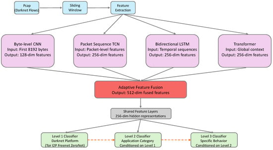
Figure 1. Overall architecture of the proposed E2E-MDC framework. The system processes raw network traffic through four specialized feature extractors (Byte-level CNN, Packet Sequence TCN, Bidirectional LSTM, and Transformer), adaptively fuses multi-modal features through attention mechanisms, and performs three-level hierarchical classification through conditional classifiers.

The system input is raw network traffic data in PCAP format, and the output consists of three hierarchical classification results: Level 1 (darknet type, such as Tor, I2P, etc.), Level 2 (application category, such as BBC, Twitter, TikTok, Telegram, Gmail, Zoom, Teams, YouTube, etc.), and Level 3 (specific application behavior, such as audio streaming, browsing, video streaming, etc.). This hierarchical classification system not only conforms to the natural hierarchical structure of darknet traffic but also provides threat intelligence at different granularities for network security analysis.

In terms of data flow processing, the system first segments continuous network traffic into fixed-size traffic segments through a sliding window mechanism. Each segment contains 2000 packets, with an overlap of 500 packets between adjacent segments. This design ensures sufficient contextual information while enabling near-real-time traffic detection. For each traffic segment, the system simultaneously extracts four types of features at different granularities: raw byte sequences, packet-level statistical features, temporal dependencies, and global semantic information.

Multi-modal feature extraction is one of the core innovations of this system. Unlike existing methods that focus only on a single type of feature, we designed four specialized deep neural network modules to capture different aspects of traffic features: (1) the byte-level CNN module directly processes the first 8192 raw bytes, extracting byte pattern features through multi-scale convolution; (2) the packet sequence TCN module processes sequence features such as packet size, direction, and time interval, using temporal convolutional networks to capture local temporal patterns; (3) the bidirectional LSTM module models long-range temporal dependencies, learning dynamic evolution features of traffic through gating mechanisms and self-attention mechanisms; and (4) the Transformer module understands the semantic information of the entire traffic segment from a global perspective, capturing complex interaction relationships between packets through multi-head attention mechanisms.

The feature fusion stage adopts an adaptive weighting mechanism. The system learns the importance weights of each feature module, dynamically adjusting the contribution of different modal features. This design enables the model to automatically select the most discriminative feature combinations based on different types of traffic. For example, for highly encrypted traffic where byte-level features may contain limited information, the system will automatically increase the weights of temporal and statistical features.

Finally, the conditional hierarchical classifier performs three-level classification decisions based on the fused features. Unlike traditional flat classification, our classifier explicitly models the conditional dependencies between different levels: Level 2 classification is conditioned on Level 1 prediction results, and Level 3 classification considers both Level 1 and Level 2 information. This conditional design not only improves classification accuracy but also ensures hierarchical consistency of prediction results.

The entire system adopts end-to-end training, with all modules jointly optimized through a unified loss function. The loss function contains three parts: weighted classification loss ensures classification accuracy at each level, hierarchical consistency loss maintains logical reasonableness of prediction results, and feature diversity regularization prevents different feature extractors from learning redundant information. This carefully designed training strategy enables system components to cooperate with each other and jointly improve overall performance.

It is worth noting that the system design fully considers the needs of practical deployment. Through modular architecture design, the system can be flexibly adjusted according to different application scenarios. For example, on edge devices with limited computational resources, certain feature extraction modules can be selectively disabled; in scenarios with high real-time requirements, the size and stride of the sliding window can be adjusted. This flexibility gives the system good practicality and scalability.

3.3. Data Preprocessing Pipeline

Data preprocessing is a key step in ensuring the performance of end-to-end learning systems. This section details our designed preprocessing pipeline, including the sliding window mechanism and multi-scale feature normalization strategy.

3.3.1. Sliding Window Mechanism

When processing network traffic data, a core challenge is how to handle variable-length traffic sequences. Traditional methods typically use complete flows or fixed time windows, but both approaches have obvious defects: the complete flow method requires the flow to end before classification, which cannot meet real-time detection requirements; fixed time windows may truncate important traffic patterns. To address this, we propose a sliding window mechanism based on a fixed number of packets.

Specifically, we segment continuous network traffic into windows containing 2000 packets, with an overlap of 500 packets between adjacent windows, i.e., a sliding stride of 1500 packets. The selection of window size and stride involves trade-offs among protocol characteristics, computational constraints, and real-time requirements.

From the perspective of traffic pattern characteristics, different application behaviors exhibit varying temporal spans. At the protocol level, fundamental operations such as TCP handshake and TLS negotiation typically complete within 10–50 packets. At the application level, interactive applications (e.g., browsing, chat) exhibit request-response patterns spanning 50–300 packets; streaming media applications establish stable transmission patterns over hundreds to thousands of packets; file transfer applications may require even longer observation sequences to manifest complete characteristics. Furthermore, the multi-layer encryption in darknet traffic causes behavioral patterns to become more dispersed, necessitating longer sequences to accumulate sufficient statistical features. Based on these considerations, a reasonable range for window size is approximately 1000–3000 packets.

Within this range, the specific choice requires consideration of practical system constraints. From a computational efficiency perspective, our framework incorporates a Transformer module whose self-attention mechanism has $O\left(n^2\right)$ complexity; when the window size increases to 3000 packets, computational overhead increases significantly, affecting real-time processing capability. From a latency perspective, in typical gigabit network environments, 1000–2000 packets correspond to approximately 1–3 s of traffic accumulation, meeting real-time monitoring requirements, whereas exceeding 2500 packets may result in excessive detection delay. From a feature completeness perspective, our preliminary experiments indicate that windows of 1500–2000 packets adequately capture behavioral characteristics for the eight categories of interest (browsing, chat, file transfer, P2P, audio/video streaming, VoIP), with diminishing performance gains from further window enlargement.

Considering these factors comprehensively, we select 2000 packets as the window size for this study. This choice performs well on our datasets, though we note that other window sizes (e.g., 1500 or 2500) may be equally or more effective under different application scenarios or network conditions.

To prevent critical behavioral patterns from being truncated at window boundaries, we introduce overlap between adjacent windows, setting the stride to 1500 packets (i.e., 25% overlap). This configuration is based on the following trade-offs: moderate overlap ensures that patterns spanning boundaries can be captured more completely in at least one window, while avoiding redundant computation from excessive overlap. This parameter setting works well in our experiments but can be adjusted according to specific requirements—latency-sensitive scenarios may reduce overlap, while scenarios demanding extreme accuracy may increase it.

The sliding window implementation also considers boundary case handling. For traffic segments with fewer than 2000 packets, we adopt a zero-padding strategy, filling insufficient parts with zero values while maintaining the original packet order. This processing ensures consistency of model input while allowing the model to identify the actual number of valid packets through packet count features.

This sliding window mechanism provides a principled approach to partitioning variable-length traffic streams while balancing pattern completeness and real-time performance.

3.3.2. Feature Normalization Strategy

Raw network traffic data contains multiple types of features with vastly different numerical ranges. Direct input to neural networks would lead to training instability. Therefore, we designed corresponding normalization strategies for different types of features.

Timestamp normalization is one of the most critical steps in preprocessing. The timestamps in raw PCAP files are absolute Unix times, and direct use would cause the model to overfit specific time periods. We convert all timestamps to relative times, using the first non-zero timestamp in each window as the reference point. The specific calculation formula is

$$\mathrm{Relative}\mathrm{timestamp}={\displaystyle \frac{\mathrm{Absolute}\mathrm{timestamp}-\mathrm{First}\mathrm{packet}\mathrm{timestamp}}{\mathrm{Window}\mathrm{time}\mathrm{span}}}.$$

(4)

This normalization method maps all timestamps to the [0, 1] interval, making the model focus on inter-packet time interval patterns rather than absolute time.

Byte sequence normalization processes raw byte data. We extract the first 8192 bytes of each traffic window as byte-level features, dividing each byte value by 255 to map to the [0, 1] interval. This simple linear normalization preserves the relative relationships between byte values, enabling the byte-level CNN to effectively learn protocol features and encryption patterns.

Packet size normalization considers the physical limitations of Ethernet. Since the Ethernet MTU is typically 1500 bytes, we normalize all packet sizes by dividing by 1500. For jumbo frames, the normalized value may be slightly larger than 1, but this situation is rare and does not significantly affect model training.

Time interval normalization adopts logarithmic scale transformation. The distribution of inter-packet time intervals in network traffic is extremely uneven, spanning multiple orders of magnitude from microseconds to seconds. Direct normalization would compress the differences between small intervals. We adopt the following logarithmic normalization strategy:

$$\mathrm{Normalized}\mathrm{interval}={\displaystyle \frac{log(1+\mathrm{interval}\mathrm{time}\times 1000)}{log(1+10000)}}.$$

(5)

This transformation maps time intervals to the [0, 1] interval while preserving the discrimination of intervals at different scales.

Protocol feature processing includes TCP flags, window size, IP flags, and TTL. TCP flags and IP flags maintain their original integer encoding and are input to the embedding layer as categorical features. TCP window size is normalized by dividing by 32,768 ($2^{15}$). TTL values maintain their original range [0, 255], as different TTL values inherently have categorical feature characteristics.

Direction feature encoding is used to distinguish the bidirectionality of traffic. We use the source IP of the first packet in each window as the client standard, marking subsequent packets as client-to-server (+1), server-to-client ($-1$), or retransmission in the same direction (0). This encoding method is simple and effective, capable of capturing traffic interaction patterns.

Additionally, we implemented data augmentation strategies to improve the model’s generalization ability. Augmentation operations include (1) time shifting: adding random perturbations of −10% to +10% to time-related features; (2) packet size perturbation: adding 5% Gaussian noise to simulate network jitter; (3) random packet loss: randomly setting certain packet features to zero with a probability of 5–15%, simulating network packet loss; and (4) byte sequence noise: adding 2% uniform noise to raw bytes, enhancing the model’s robustness to slight content changes.

All preprocessing operations are carefully designed to ensure that while improving model training stability, key information in the original traffic is not lost. The preprocessed data is input to subsequent feature extraction modules in standardized tensor format, laying a solid foundation for end-to-end learning.

3.4. Multi-Modal Feature Extraction

Multi-modal feature extraction is the core innovation of this system, capturing features of darknet traffic from different perspectives through four specially designed deep neural network modules. Each module is optimized for specific types of information, collectively forming a comprehensive feature representation system.

3.4.1. Byte-Level CNN Module

The byte-level CNN module directly processes the byte sequence of raw traffic, aiming to automatically learn protocol features, encryption patterns, and application fingerprints. The module input is the first 8192 bytes of each traffic window, and the output is a 128-dimensional feature vector. This design draws on the idea of Network in Network [26].

The first layer of the module is a byte embedding layer, mapping each byte (0–255) to a 32-dimensional dense vector space. This embedding representation is more compact than one-hot encoding and can learn semantic similarity between bytes. For example, bytes within the ASCII character range may be mapped to similar embedding spaces, while random bytes of encrypted data are distributed more uniformly. The byte-level CNN architecture is shown in Figure 2.

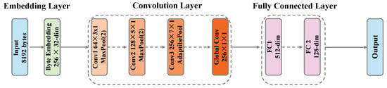
Figure 2. Architecture of the byte-level CNN module. The module processes 8192 raw bytes through embedding layer, three multi-scale convolutional blocks, and fully connected layers to extract 128-dimensional byte pattern features.

The core feature extraction adopts a three-layer multi-scale convolution structure:

The first convolution layer uses 64 $3\times 1$ convolution kernels, combined with batch normalization and ReLU activation function, mainly capturing local patterns between adjacent bytes. This layer is followed by $2\times$ max pooling, halving the sequence length to 4096. This design can effectively identify short-range protocol identifiers and fixed header patterns.

The second convolution layer uses 128 $5\times 1$ convolution kernels, with a receptive field expanded to 5 bytes, capable of capturing longer byte patterns such as HTTP request methods and TLS handshake messages. Similarly using batch normalization, ReLU activation, and $2\times$ max pooling, the sequence length is further reduced to 2048.

The third convolution layer uses 256 $7\times 1$ convolution kernels with a larger receptive field for capturing complex patterns of application layer protocols. This layer is followed by adaptive max pooling, uniformly compressing feature sequences of different lengths to a fixed length of 64, ensuring consistency in subsequent processing.

After multi-scale convolution, we add a global convolution layer using 256 $1\times 1$ convolution kernels to transform features at each position. This design draws on the idea of Network in Network, enhancing the model’s nonlinear expressive power.

Finally, the extracted features are projected to a 128-dimensional output space through a two-layer fully connected network. The first fully connected layer maps the flattened $256\times 64$ = 16,384-dimensional features to 512 dimensions, combined with batch normalization, ReLU activation, and 0.2 dropout to prevent overfitting. The second fully connected layer outputs the final 128-dimensional feature representation.

3.4.2. Packet Sequence Temporal Convolutional Network (TCN)

The packet sequence TCN module [27] specifically processes packet-level statistical feature sequences, including 7-dimensional features such as packet size, direction, time interval, TCP flags, window size, IP flags, and TTL. The module adopts a temporal convolutional network architecture and outputs a 256-dimensional feature vector. The packet sequence TCN architecture is shown in Figure 3.

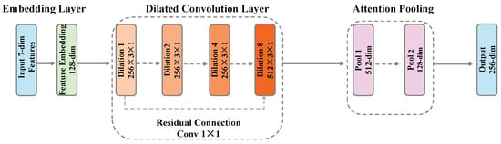
Figure 3. Architecture of the packet sequence TCN module. The module employs dilated causal convolutions with exponentially growing dilation rates (1, 2, 4, 8) to capture multi-scale temporal patterns from packet sequences.

Feature embedding is the first step of this module. Different types of features adopt different embedding strategies: continuous value features (packet size, time interval, window size) are mapped to 32-dimensional spaces through linear transformation respectively; discrete features (direction, TCP flags, IP flags, TTL) learn their semantic representations through embedding layers. All embedded features are concatenated into a unified 128-dimensional representation.

The core TCN structure adopts 4 layers of dilated convolution with dilation rates of 1, 2, 4, and 8 respectively. This exponentially growing dilation rate enables the network to obtain a large receptive field with fewer layers. The design of each layer is as follows:

• Layer 1: 256 $3\times 1$ convolution kernels, dilation rate 1, capturing direct relationships between adjacent packets
• Layer 2: 256 $3\times 1$ convolution kernels, dilation rate 2, capturing patterns with 1-packet intervals
• Layer 3: 256 $3\times 1$ convolution kernels, dilation rate 4, capturing larger-range temporal patterns
• Layer 4: 512 $3\times 1$ convolution kernels, dilation rate 8, capturing long-range dependencies

Each layer includes batch normalization, ReLU activation, and 0.1 dropout. To address the vanishing gradient problem, we add residual connections between Layer 1 and Layer 4, projecting the 128-dimensional input to 512 dimensions through $1\times 1$ convolution and adding it to the Layer 4 output.

An innovation point of this module is the attention pooling mechanism. Traditional global average pooling or max pooling may lose important local information. We designed a two-layer attention network: the first layer compresses 512-dimensional features to 128 dimensions and uses Tanh activation, and the second layer outputs 1-dimensional attention scores. After Softmax normalization, these scores serve as weights to perform weighted summation of features at different time steps, obtaining the final 512-dimensional aggregated features. Finally, the 256-dimensional packet sequence feature representation is output through linear projection.

3.4.3. Bidirectional LSTM with Attention Module

The bidirectional LSTM module focuses on modeling the temporal dynamic characteristics of traffic, particularly long-range dependencies in packet sequences. This module also takes 7-dimensional packet-level features as input and outputs a 256-dimensional feature vector. The bidirectional LSTM architecture is shown in Figure 4.

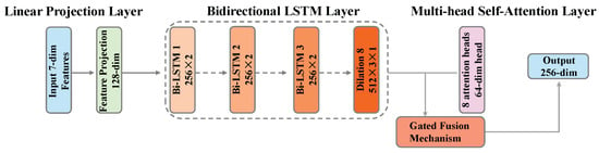
Figure 4. Architecture of the bidirectional LSTM module. The module processes packet sequences through 3-layer bidirectional LSTM, applies multi-head self-attention, and fuses features through a gating mechanism.

Input features are first expanded to 128 dimensions through a linear projection layer, providing richer input representation for LSTM. The core network is a 3-layer bidirectional LSTM with a hidden dimension of 256 in each direction, totaling 512 hidden dimensions. Using multi-layer LSTM can learn more complex temporal patterns, while the bidirectional structure allows the model to utilize both past and future contextual information simultaneously. Inter-layer dropout is set to 0.2 to prevent overfitting.

Based on LSTM output, we introduce a self-attention mechanism to further refine features. Specifically, 8-head attention is used, with each head focusing on a 64-dimensional subspace. This multi-head design allows the model to focus on different parts of the sequence from different angles. Attention calculation follows the standard scaled dot-product attention formula with 0.1 dropout added to improve generalization.

A key innovation is the gated fusion mechanism. LSTM output and attention output are adaptively fused through a gating network. The gating network generates 512-dimensional gate values through a linear layer and Sigmoid activation function on the concatenated 1024-dimensional features (512-dimensional LSTM + 512-dimensional attention), controlling the mixing ratio of the two types of features:

$$\mathrm{Fused}\mathrm{feature}=g\odot \mathrm{LSTM}\mathrm{output}+(1-g)\odot \mathrm{Attention}\mathrm{output},$$

(6)

where g represents the gate values and ⊙ denotes element-wise multiplication. This design enables the model to adaptively choose to rely on LSTM’s temporal modeling or attention’s global correlation based on input characteristics.

The final feature representation is obtained through two methods: one is the hidden state at the last time step of LSTM (considering bidirectionality, concatenating the final hidden states of forward and backward directions), and the other is average pooling of fused features at all time steps. After averaging the two, they are projected to the 256-dimensional output space through a multi-layer perceptron containing batch normalization, ReLU, and dropout.

3.4.4. Transformer Global Feature Extractor

The Transformer module understands the semantic information of the entire traffic window from a global perspective, capturing complex interaction relationships between packets through self-attention mechanisms. This module also processes 7-dimensional packet features and outputs a 256-dimensional feature vector. The Transformer architecture is shown in Figure 5.

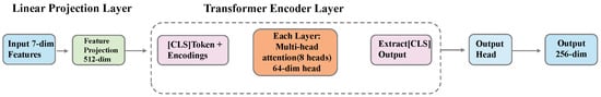
Figure 5. Architecture of the Transformer module. The module introduces a [CLS] token to aggregate global information and processes the sequence through 6 Transformer encoder layers with multi-head self-attention.

The input 7-dimensional features are first expanded to the 512-dimensional model dimension ($d_{\mathrm{model}}$) through linear projection. Unlike the standard Transformer, we use learnable positional encoding rather than fixed sinusoidal encoding, allowing the model to adaptively learn positional patterns in darknet traffic. Positional encoding is a learnable parameter with shape [1, 2000, 512], added directly to the input embeddings.

The adoption of learnable positional encoding is a deliberate design choice motivated by the unique characteristics of encrypted network traffic classification. This approach offers three key advantages over fixed sinusoidal encoding.

First, domain-specific adaptivity: Learnable encoding enables the model to discover and represent the temporal patterns inherent in darknet traffic through end-to-end training. Encrypted network packets exhibit irregular timing distributions, protocol-specific ordering patterns, and burst transmission behaviors that differ fundamentally from the sequential structures found in natural language or other domains where fixed sinusoidal encoding was originally designed. By parameterizing the positional embeddings as learnable weights, the model can adapt to these domain-specific characteristics rather than imposing predetermined periodic patterns.

Second, task-driven optimization: Through joint training with the hierarchical classification objective, the learnable positional embeddings are optimized to encode position information that is most discriminative for distinguishing darknet applications and behaviors. This end-to-end learning allows the model to automatically identify which positional features are relevant for classification while discarding irrelevant temporal variations. The gradient flow from classification loss directly shapes the positional representations, ensuring they contribute effectively to the final prediction rather than serving as generic position markers.

Third, multi-scale temporal modeling: Darknet traffic patterns manifest across multiple temporal scales—from microsecond-level inter-packet intervals to second-level session dynamics. Learnable encoding provides the flexibility to adaptively weight different temporal granularities based on their relevance to each hierarchical classification level. For instance, fine-grained Level 3 behavior classification may rely more heavily on short-range temporal patterns, while Level 2 application identification may benefit from longer-range dependencies. The learnable nature of positional embeddings allows such task-specific temporal focusing to emerge naturally during training.

Furthermore, the learnable encoding maintains compatibility with the overall architecture’s differentiability, enabling seamless gradient backpropagation throughout the entire model. This is particularly important for our conditional hierarchical classification framework, where optimization signals must flow across multiple classification levels and feature modalities.

To enhance the model’s perception of different stages of traffic, we introduce a segment embedding mechanism. The sequence of 2000 packets is divided equally into three segments, the beginning segment (first 667 packets), middle segment (668–1334 packets), and ending segment (last 666 packets), each identified with different segment embedding vectors. This design helps the model distinguish different stages of traffic, such as handshake phase, data transmission phase, and termination phase.

The [CLS] token mechanism is a key innovation of this module. Drawing on the design idea of BERT [28], we add a special [CLS] (Classification) token at the beginning of each input sequence. This token is a learnable parameter vector, initialized as a 512-dimensional random vector, consistent with the model dimension.

The design of the [CLS] token has several important considerations:

First, it provides a dedicated “anchor point” to aggregate global information. During self-attention computation, the [CLS] token can interact with all packets in the sequence, but it does not carry information about any specific packet itself, thus being able to neutrally learn the global representation of the entire sequence. This is particularly important for darknet traffic classification, as judging traffic type often requires comprehensive consideration of the entire communication pattern rather than local features.

Second, through 6-layer Transformer encoding, the [CLS] token aggregates information layer by layer. In shallow layers, it mainly focuses on local patterns between adjacent packets; in deep layers, as the receptive field expands, it can capture more complex global interaction patterns. The self-attention mechanism at each layer allows the [CLS] token to selectively focus on different parts of the sequence based on the current representation.

In specific implementation, the input sequence is expanded from the original [batch_size, 2000, 512] to [batch_size, 2001, 512], where position 0 is the [CLS] token. When applying positional encoding, we assign position 0 to the [CLS] token, and the positions of the original sequence are shifted backward accordingly. This processing ensures continuity of positional information.

The core Transformer encoder contains 6 layers, each consisting of multi-head self-attention and feed-forward network. Specific configuration is as follows:

• Number of attention heads: 8;
• Dimension per head: 64 (total 512 dimensions);
• Feed-forward network dimension: 2048;
• Activation function: GELU;
• Dropout rate: 0.1.

In self-attention computation, the [CLS] token participates in all attention calculations. It both attends to other positions as a query and is attended to by other positions as key and value. This bidirectional interaction enables the [CLS] token to effectively integrate global information. In particular, since darknet traffic often contains encrypted content, individual packet information may be limited, but the overall pattern of packet sequences (such as packet size distribution, time interval regularity, etc.) can reveal application types. The [CLS] token is the ideal carrier for capturing such overall patterns.

After 6 layers of encoding, we extract the output at the [CLS] position (i.e., position 0) as the representation of the entire sequence. This 512-dimensional vector contains the Transformer’s understanding of the traffic window from a global perspective. Compared to simple average pooling or max pooling, the [CLS] token provides a more flexible and powerful sequence representation method.

The final output head is a two-layer network containing layer normalization, ReLU activation, and dropout. The first layer maintains 512 dimensions for feature transformation and regularization; the second layer projects the dimension to 256 dimensions, consistent with the output of other feature extraction modules. This design ensures feature compatibility, facilitating subsequent multi-modal fusion.

It is worth noting that although the computational complexity of Transformer is high ($O\left(n^2\right)$ relative to sequence length), in our application scenario, the fixed window size of 2000 packets makes the computational cost controllable. Meanwhile, the [CLS] token mechanism avoids the need to pool outputs at all positions, improving computational efficiency.

The four feature extraction modules capture features of darknet traffic from different perspectives: the byte-level CNN focuses on underlying protocol and encryption patterns, the packet sequence TCN extracts local temporal patterns, the bidirectional LSTM models long-range dependencies, and the Transformer provides global semantic understanding through the [CLS] token. This multi-modal design ensures feature comprehensiveness and complementarity, providing a rich information foundation for subsequent classification tasks.

3.5. Adaptive Feature Fusion

The adaptive feature fusion module is the key bridge connecting multi-modal feature extraction and conditional hierarchical classification. This module does not simply concatenate features from different modalities but learns the importance of each modality through attention mechanisms and captures interactions between modalities through cross-attention, ultimately generating a unified 512-dimensional feature representation.

3.5.1. Attention-Driven Weighting Mechanism

The first step of feature fusion is projecting features from four different modalities into a unified representation space. Although the byte-level CNN outputs 128 dimensions and the other three modules output 256 dimensions, their semantic spaces differ. Through independent linear projection layers, we map all features to a shared 256-dimensional space:

• Byte features: $128\to 256$ dimensions (expansion projection);
• TCN features: $256\to 256$ dimensions (semantic alignment);
• LSTM features: $256\to 256$ dimensions (semantic alignment);
• Transformer features: $256\to 256$ dimensions (semantic alignment).

This projection not only unifies dimensions but more importantly learns a shared semantic space, enabling features from different modalities to be compared and fused at the same scale.

Next is the calculation of attention weights. We designed a two-layer attention network to learn the importance of each modality. First, the four projected features are concatenated into a 1024-dimensional vector and input to the first fully connected network ($1024\to 256$), using Tanh activation function to introduce nonlinearity. The second layer ($256\to 4$) outputs four scalar values, corresponding to the importance scores of the four modalities.

The key insight of this design is that different types of darknet traffic may depend on different feature modalities. For example,

• For highly encrypted traffic, byte-level features may contain limited information, making temporal features more important.
• For applications with obvious interaction patterns (such as chat), LSTM and Transformer features may be more discriminative.
• For streaming media applications, statistical features of packet sequences (TCN) may be most critical.

Through Softmax normalization, the four importance scores are converted into a probability distribution totaling 1, serving as weights for each modality. Each modality’s feature vector is multiplied by its corresponding weight to obtain weighted feature representations. This soft selection mechanism is more flexible than hard feature selection, allowing the model to dynamically adjust its dependence on different modalities based on input.

3.5.2. Cross-Modal Attention Mechanism

Simply weighting and summing features ignores potential complex interaction relationships between modalities. To address this, we introduce a cross-attention mechanism that allows features from different modalities to mutually enhance each other.

In specific implementation, we stack the four weighted feature vectors into a tensor with shape [batch_size, 4, 256], where 4 represents the number of modalities. This tensor is input to a multi-head attention layer with the following configuration:

• Embedding dimension: 256;
• Number of attention heads: 8;
• Dimension per head: 32;
• Dropout rate: 0.1.

In this cross-attention computation, features from each modality serve both as queries to attend to other modalities and as keys and values to be attended to by other modalities. This mechanism allows the model to learn complementary relationships between modalities. For example,

• Byte-level features may gain global context by attending to Transformer features;
• LSTM features may enhance understanding of local patterns by attending to TCN features;
• Transformer features may refine identification of specific protocols by attending to byte-level features.

The output of cross-attention maintains the shape [batch_size, 4, 256], containing feature representations enhanced through inter-modal interaction. These features not only retain unique information from each modality but also incorporate complementary information from other modalities.

Finally, the output of cross-attention is flattened into a 1024-dimensional vector and input to a three-layer fully connected network for final feature fusion:

• First layer: $1024\to 1024$ dimensions, with batch normalization, ReLU activation, and 0.3 dropout.
• Second layer: $1024\to 512$ dimensions, with batch normalization, ReLU activation, and 0.2 dropout.
• Third layer: $512\to 512$ dimensions, outputting the final fused features.

This multi-layer perceptron not only completes dimension transformation but more importantly learns a nonlinear feature combination function that can capture high-order interactions between different modal features. Higher dropout rates (0.3 and 0.2) ensure that the model does not overly depend on specific feature combinations, improving generalization ability.

The fused 512-dimensional feature vector contains comprehensive information from four modalities, both retaining the unique contribution of each modality and achieving adaptive feature selection and interaction through attention mechanisms. This unified representation will be sent to the conditional hierarchical classifier to complete the final classification task.

An important characteristic of the entire fusion process is end-to-end learnability. Attention weights, cross-attention parameters, and fusion network are all jointly optimized through backpropagation, enabling the fusion strategy to automatically adapt to different data distributions and classification tasks. Meanwhile, attention weights generated during the fusion process also provide important clues for model interpretability, helping us understand from which modalities the discriminative features of different types of traffic mainly come.

3.6. Conditional Hierarchical Classifier

The conditional hierarchical classifier is the core component for achieving precise three-level classification in this system. Unlike traditional flat classification or independent multi-task learning, this classifier explicitly models the conditional dependencies between the three classification levels, ensuring prediction results are both accurate and comply with hierarchical logic.

3.6.1. Hierarchical Structure Design

The classifier input is a 512-dimensional feature vector from the feature fusion module, and it needs to simultaneously output classification results at three levels: Level 1 (darknet type), Level 2 (application category), and Level 3 (specific behavior). Our hierarchical architecture includes a shared feature extraction layer and three conditioned classification heads.

The shared feature extraction layer is responsible for further extracting high-level semantic representations related to classification tasks from fused features. This layer consists of two fully connected blocks:

• First fully connected block: $512\to 256$ dimensions, followed by batch normalization, ReLU activation, and 0.3 dropout. This layer compresses fused features to a more compact representation space while preventing overfitting through higher dropout rates.
• Second fully connected block: $256\to 256$ dimensions, also equipped with batch normalization, ReLU activation, and 0.3 dropout. This layer further refines features while maintaining dimensionality, learning representations more suitable for hierarchical classification.

The design of the shared layer is based on the assumption that although the three-level classification tasks are different, they share certain fundamental discriminative features. Through shared feature extraction, the model can more effectively utilize limited training data while ensuring consistency of predictions at different levels.

The Level 1 classification head is the simplest because it does not depend on information from other levels. This classification head contains two layers:

• First layer: $256\to 128$ dimensions, batch normalization + ReLU + 0.3 dropout;
• Second layer: $128\to n_1$ dimensions, outputting classification logits for Level 1.

In our experiments, Level 1 includes 4 classes (Tor, I2P, Freenet, ZeroNet) or 1 class (only self-collected Tor data). This layer mainly identifies the type of darknet technology used.

The innovation of the Level 2 classification head lies in its conditioning on Level 1 prediction results. Specifically, Level 1 output logits are converted to probability distribution through Softmax and then concatenated with shared features to form conditional features of $(256+n_1)$ dimensions. This design enables Level 2 predictions to consider Level 1 uncertainty:

• Input: [Shared features (256 dim), Level 1 probabilities ($n_1$ dim)];
• First layer: $(256+n_1)\to 128$ dimensions, batch normalization + ReLU + 0.3 dropout;
• Second layer: $128\to n_2$ dimensions, outputting classification logits for Level 2.

Using probabilities rather than hard classification results as conditions has two advantages: first, it retains the uncertainty information from Level 1 predictions; second, it makes the entire network end-to-end trainable, allowing gradients to backpropagate through the Softmax operation to Level 1.

The Level 3 classification head further extends the conditionalization idea by simultaneously considering Level 2 prediction results:

• Input: [Shared features (256 dim), Level 2 probabilities ($n_2$ dim)];
• First layer: $(256+n_2)\to 128$ dimensions, batch normalization + ReLU + 0.3 dropout;
• Second layer: $128\to n_3$ dimensions, outputting classification logits for Level 3.

This cascaded conditional design ensures hierarchical consistency of predictions. For example, if Level 2 predicts “Youtube”, Level 3 is more likely to predict “video” rather than “filetransfer” or “browsing”.

3.6.2. Conditional Probability Modeling

From a probabilistic perspective, our hierarchical classifier is actually modeling the joint probability distribution $P(L_1,L_2,L_3\mid X)$, where X is the input feature and $L_1,L_2,L_3$ are labels at three levels, respectively. Through conditional decomposition, we express it as

$$P(L_1,L_2,L_3\mid X)=P(L_1\mid X)\times P(L_2\mid L_1,X)\times P(L_3\mid L_2,X).$$

(7)

This decomposition not only conforms to the natural structure of hierarchical labels but also simplifies the learning task. Each classification head only needs to learn the corresponding conditional probability distribution rather than directly learning the complex joint distribution.

In implementation, conditional dependencies are embodied through the following ways:

• Feature-level conditioning: Classification heads at subsequent levels receive the probability distribution from the previous level as additional input, providing explicit conditional information.
• Implicit regularization: Through the shared feature extraction layer, classification heads at different levels are softly constrained, encouraging them to learn consistent representations.
• Loss function constraints: During training, we not only optimize classification accuracy at each level but also ensure predictions conform to predefined hierarchical structure through hierarchical consistency loss (detailed in Section 3.7).

3.6.3. Inference Strategy

During the inference stage, the classifier adopts a top-down prediction strategy:

Step 1: Level 1 Prediction. First obtain the darknet type prediction through the Level 1 classification head. Let the input feature be x, and shared feature be $h=f_{\mathrm{shared}}\left(x\right)$, then

$$\begin{array}{cc}\hfill {\mathrm{logits}}^1& =f_{\mathrm{level}1}\left(h\right),\hfill \end{array}$$

(8)

$$\begin{array}{cc}\hfill {\mathrm{probs}}^1& =\mathrm{Softmax}\left({\mathrm{logits}}^1\right),\hfill \end{array}$$

(9)

$$\begin{array}{cc}\hfill {\mathrm{pred}}^1& =argmax\left({\mathrm{probs}}^1\right).\hfill \end{array}$$

(10)

Step 2: Level 2 Conditional Prediction. Concatenate Level 1 probability distribution with shared features and input to Level 2 classification head:

$$\begin{array}{cc}\hfill {\mathrm{logits}}^2& =f_{\mathrm{level}2}\left([h,{\mathrm{probs}}^1]\right),\hfill \end{array}$$

(11)

$$\begin{array}{cc}\hfill {\mathrm{probs}}^2& =\mathrm{Softmax}\left({\mathrm{logits}}^2\right),\hfill \end{array}$$

(12)

$$\begin{array}{cc}\hfill {\mathrm{pred}}^2& =argmax\left({\mathrm{probs}}^2\right).\hfill \end{array}$$

(13)

Step 3: Level 3 Conditional Prediction. Similarly, use Level 2 probability distribution:

$$\begin{array}{cc}\hfill {\mathrm{logits}}^3& =f_{\mathrm{level}3}\left([h,{\mathrm{probs}}^2]\right),\hfill \end{array}$$

(14)

$$\begin{array}{cc}\hfill {\mathrm{probs}}^3& =\mathrm{Softmax}\left({\mathrm{logits}}^3\right),\hfill \end{array}$$

(15)

$$\begin{array}{cc}\hfill {\mathrm{pred}}^3& =argmax\left({\mathrm{probs}}^3\right).\hfill \end{array}$$

(16)

An important characteristic of this inference strategy is uncertainty propagation. When Level 1 prediction is uncertain (such as when the probability distribution is relatively uniform), this uncertainty is transmitted through the probability vector to Level 2, making its prediction more cautious. This is valuable in practical applications as it can identify difficult-to-classify boundary cases.

Another advantage is computational efficiency. Although we have three classification heads, shared features only need to be computed once, and each classification head is relatively lightweight. In our implementation, the computational overhead of the entire classification process is only slightly higher than a single three-way classifier.

Additionally, this architecture supports partial hierarchical prediction. In some application scenarios, only Level 1 or Level 1 + Level 2 prediction results may be needed. Our design allows predictions to be stopped at any level, providing flexible deployment options.

The conditional hierarchical classifier achieves accurate three-level classification through carefully designed architecture and inference strategy while ensuring hierarchical consistency of prediction results. This design is particularly suitable for darknet traffic classification tasks because strong dependencies indeed exist between labels at different levels, and our method can effectively utilize this structural information to improve classification performance.

3.7. Loss Function Design

The design of the loss function is crucial for end-to-end learning systems, as it not only guides the model to learn accurate classification boundaries but also ensures coordinated optimization of all system components. The loss function proposed in this paper consists of three carefully designed components: weighted classification loss, hierarchical consistency loss, and feature diversity regularization. This multi-objective optimization strategy enables the model to maintain hierarchical logical reasonability of predictions while ensuring classification accuracy and fully utilize the complementarity of multi-modal features.

3.7.1. Weighted Classification Loss

Weighted classification loss is the basic component of the entire loss function, responsible for optimizing classification accuracy at three levels. Considering that different levels have different classification difficulties and importance, we assign different weights to each level. In actual implementation, the weights for Level 1, Level 2, and Level 3 are set to 0.3, 0.3, and 0.4 respectively. This configuration reflects our emphasis on fine-grained classification (Level 3) while ensuring that coarse-grained classifications (Level 1 and Level 2) are also sufficiently trained.

This weight configuration reflects two design considerations: first, Level 3 behavior classification is more challenging than Level 1 platform or Level 2 application identification due to subtle distinctions under encryption, warranting higher weight (${\alpha }^{\left(3\right)}=0.4$); second, equal weighting for Level 1 and Level 2 (${\alpha }^{\left(1\right)}={\alpha }^{\left(2\right)}=0.3$) ensures reliable conditional information for the hierarchical classifier, as upper-level predictions serve as inputs for lower levels.

The specific values were determined through preliminary validation experiments, demonstrating effective balance between Level 3 optimization and foundational level performance. Comprehensive ablation of loss weights is beyond the scope of this work, as our focus is on the conditional hierarchical mechanism and multi-modal fusion strategy.

The classification loss at each level adopts cross-entropy loss function with label smoothing. Label smoothing is an effective regularization technique [29] that prevents the model from being overconfident by reducing the probability of the true label from 1.0 to $1.0-ϵ$ (where $ϵ=0.1$ in this paper) and uniformly distributing $ϵ$ to other classes, thereby improving generalization ability. This is particularly important in darknet traffic classification because some traffic samples may simultaneously have features of multiple classes, and completely hard labels may be too absolute.

For a single sample, the classification loss at level ℓ ($\mathsf{\ell }\in \{1,2,3\}$) is defined as

$${\mathcal{L}}_{\mathrm{CE}}^{(\mathsf{\ell })}=-\sum _{i=1}^{n_{\mathsf{\ell }}}{y}_i^{(\mathsf{\ell })}log\left(p_i^{(\mathsf{\ell })}\right),$$

(17)

where $y_i^{(\mathsf{\ell })}$ is the smoothed label probability for class i at level ℓ, $p_i^{(\mathsf{\ell })}$ is the predicted probability, and $n_{\mathsf{\ell }}$ is the number of classes at level ℓ. With label smoothing, the smoothed label is

$$y_i^{(\mathsf{\ell })}=\left\{\begin{array}{cc}1-ϵ+{\displaystyle \frac{ϵ}{n_{\mathsf{\ell }}}},\hfill & \mathrm{if}i=y_{\mathrm{true}}\hfill \\ {\displaystyle \frac{ϵ}{n_{\mathsf{\ell }}}},\hfill & \mathrm{otherwise}\hfill \end{array}\right.$$

(18)

The calculation of classification loss considers the class imbalance problem. Darknet traffic datasets typically suffer from severe class imbalance, with some application types (such as browsing) having far more samples than others (such as VoIP). Although we use a balanced sampler during data loading, we still retain the option of class weighting in loss calculation to provide additional safeguards for extreme imbalance situations.

The total weighted classification loss is computed as

$${\mathcal{L}}_{\mathrm{classification}}={\alpha }^{\left(1\right)}{\mathcal{L}}_{\mathrm{CE}}^{\left(1\right)}+{\alpha }^{\left(2\right)}{\mathcal{L}}_{\mathrm{CE}}^{\left(2\right)}+{\alpha }^{\left(3\right)}{\mathcal{L}}_{\mathrm{CE}}^{\left(3\right)},$$

(19)

where ${\alpha }^{\left(1\right)}=0.3$, ${\alpha }^{\left(2\right)}=0.3$, and ${\alpha }^{\left(3\right)}=0.4$ are the weights for the three levels.

3.7.2. Hierarchical Consistency Loss

Hierarchical consistency loss is one of the innovative contributions of this paper, aiming to ensure that predictions at three levels conform to predefined hierarchical structure. In darknet traffic classification, there are clear inclusion relationships between labels at different levels: specific Level 2 categories can only appear under specific Level 1 categories, and similarly, specific Level 3 categories can only correspond to specific Level 2 categories. Predictions that violate this hierarchical relationship are not only logically unreasonable but also cause confusion in practical applications.

Hierarchical consistency loss is implemented through soft constraints. For each training sample, we first obtain prediction probability distributions at three levels. Then, based on predefined hierarchical mapping relationships (${\phi }_{21}$: Level 2 to Level 1 mapping, and ${\phi }_{32}$: Level 3 to Level 2 mapping), we calculate the consistency degree of predictions. Specifically, if the model predicts a high probability for a certain Level 2 class for a sample, the prediction probability for its corresponding Level 1 parent class should also be correspondingly high.

The hierarchical consistency loss between Level 2 and Level 1 is defined as

$${\mathcal{L}}_{\mathrm{cons}}^{(2\to 1)}=\sum _{j=1}^{n_2}{p}_j^{\left(2\right)}{\left(p_j^{\left(2\right)}-p_{{\phi }_{21}\left(j\right)}^{\left(1\right)}\right)}^2,$$

(20)

where $p_j^{\left(2\right)}$ is the predicted probability for Level 2 class j, and $p_{{\phi }_{21}\left(j\right)}^{\left(1\right)}$ is the predicted probability for its corresponding Level 1 parent class.

Similarly, the hierarchical consistency loss between Level 3 and Level 2 is

$${\mathcal{L}}_{\mathrm{cons}}^{(3\to 2)}=\sum _{k=1}^{n_3}{p}_k^{\left(3\right)}{\left(p_k^{\left(3\right)}-p_{{\phi }_{32}\left(k\right)}^{\left(2\right)}\right)}^2.$$

(21)

The total hierarchical consistency loss is

$${\mathcal{L}}_{\mathrm{consistency}}={\displaystyle \frac{1}{2}}\left({\mathcal{L}}_{\mathrm{cons}}^{(2\to 1)}+{\mathcal{L}}_{\mathrm{cons}}^{(3\to 2)}\right).$$

(22)

In implementation, we use mean squared error (MSE) to measure this consistency. For each Level 2 category prediction, we check the prediction probability of its corresponding Level 1 parent category and calculate the difference between them. This soft constraint is more flexible than hard logical rules, allowing the model to maintain certain prediction diversity in uncertain situations while maintaining hierarchical consistency overall.

The weight of hierarchical consistency loss is set to ${\lambda }_{\mathrm{consistency}}=0.1$. This relatively small weight ensures that it serves as an auxiliary objective without excessively interfering with the main classification task. During training, we observed that this loss term has significant effect in the early training phase, helping the model quickly learn hierarchical structure; in later stages, when the model has internalized the hierarchical relationships, its value is usually very small, mainly serving a maintenance role.

3.7.3. Feature Diversity Regularization

Feature diversity regularization is an innovative loss term designed for multi-modal fusion. A common problem in multi-modal learning is that different feature extractors may learn similar or redundant representations, which not only wastes model capacity but may also lead to overfitting. Feature diversity regularization addresses this problem by encouraging different modalities to learn complementary features.

This loss term is based on attention weights in the feature fusion module. Ideally, if all four feature extractors (byte-level CNN, packet sequence TCN, bidirectional LSTM, and Transformer) learn valuable and complementary features, the attention weights during fusion should be relatively balanced. Conversely, if the weight of a certain modality approaches 1 while others approach 0, it indicates that the model overly depends on a single modality and does not fully utilize the advantages of multi-modality.

We use KL divergence to measure the difference between the actual attention distribution and uniform distribution. Let $\mathbf{w}$ = $[w_1,w_2,w_3,w_4]$ denote the attention weights for the four modalities (where ${\sum }_{i=1}^4{w}_i=1$), and $\mathbf{u}=[0.25,0.25,0.25,0.25]$ denote the uniform distribution. The feature diversity regularization is defined as

$${\mathcal{L}}_{\mathrm{diversity}}=\mathrm{KL}(\mathbf{w}\parallel \mathbf{u})=\sum _{i=1}^4{w}_{i}log\left({\displaystyle \frac{w_i}{0.25}}\right).$$

(23)

This loss term encourages the model to utilize all modalities equally when possible but still allows unbalanced weights in specific situations (such as when certain modalities are indeed more informative).

The weight of feature diversity regularization is set to ${\lambda }_{\mathrm{diversity}}=0.01$. This very small weight ensures it only plays a slight regularization role and does not force the model to use equal attention weights in all situations. In practice, we found that this loss term effectively prevents the model from degenerating into extreme cases of single-modality dependence while retaining the flexibility to adaptively adjust weights based on input.

3.7.4. Total Loss Function

The total loss function is the weighted sum of three components:

$${\mathcal{L}}_{\mathrm{total}}={\mathcal{L}}_{\mathrm{classification}}+{\lambda }_{\mathrm{consistency}}{\mathcal{L}}_{\mathrm{consistency}}+{\lambda }_{\mathrm{diversity}}{\mathcal{L}}_{\mathrm{diversity}},$$

(24)

where ${\lambda }_{\mathrm{consistency}}=0.1$ and ${\lambda }_{\mathrm{diversity}}=0.01$ are the weights for hierarchical consistency loss and feature diversity regularization, respectively.

Expanding the classification loss term, we have

$${\mathcal{L}}_{\mathrm{total}}=\sum _{\mathsf{\ell }=1}^3{\alpha }^{(\mathsf{\ell })}{\mathcal{L}}_{\mathrm{CE}}^{(\mathsf{\ell })}+{\lambda }_{\mathrm{consistency}}{\mathcal{L}}_{\mathrm{consistency}}+{\lambda }_{\mathrm{diversity}}{\mathcal{L}}_{\mathrm{diversity}}.$$

(25)

This weight configuration has been validated through extensive experiments, effectively introducing constraints on hierarchical consistency and feature diversity while ensuring main classification task performance.

During training, all loss components are jointly optimized through automatic differentiation framework. Gradients backpropagate from the total loss to all trainable parameters, including four feature extractors, the feature fusion module, and the conditional hierarchical classifier. This end-to-end training approach ensures coordinated optimization of system components, enabling them to cooperate with each other and jointly improve overall performance.

The loss function design also considers training stability. By using label smoothing, appropriate loss weights, and gradient clipping (set to 1.0 in the optimizer), we ensure smooth convergence of the training process. In actual training, we monitor the change trends of each loss component to ensure they all decrease within reasonable ranges, without situations where a certain component dominates training or is ignored.

4. Experimental Evaluation and Analysis

4.1. Experimental Setup

4.1.1. Dataset Description

This study employs two representative darknet traffic datasets for experimental validation to comprehensively evaluate the effectiveness and robustness of the proposed method across different traffic scenarios. The first dataset is a combination of the publicly available Darknet-2020 [10] and CIC-Darknet2020 [8] datasets, which were collected and published by Shanghai Jiao Tong University and the Canadian Institute for Cybersecurity, respectively. These datasets contain traffic data from four mainstream darknet platforms: Tor, I2P, Freenet, and ZeroNet. The traffic covers 8 typical application behavior categories: audio streaming (audio), web browsing (browsing), instant chat (chat), email (email), file transfer (filetransfer), peer-to-peer communication (p2p), video streaming (video), and voice over IP (voip). The diversity of this dataset makes it an important benchmark for evaluating darknet traffic classification methods, with Tor traffic accounting for the majority, reflecting the widespread use of the Tor network in the real world.

The second dataset is our self-collected Tor traffic dataset, specifically designed to verify the model’s fine-grained classification capability on a specific darknet platform. The dataset was collected between March and May 2025 using three identical desktop computers (Intel Core i7-11700K, Intel Corporation, Chengdu, China, 32 GB RAM, Ubuntu 22.04 LTS) installed with the latest stable version of Tor Browser. At the time of collection, only two pluggable transports were officially supported by the Tor network: WebTunnel and obfs4. Both protocols were utilized during the data capture process to ensure comprehensive coverage of current Tor traffic characteristics.

We developed a custom Python-based traffic capture script built on tshark and pyshark libraries. The script monitors the process ID of target browser windows to enable precise isolation of traffic from individual applications. Traffic filtering is applied at three levels. First, protocol filtering captures only TCP traffic associated with Tor circuits. Second, port filtering isolates traffic on Tor’s default SOCKS port and bridge ports. Third, process filtering binds captures to specific browser window PIDs to ensure single-application isolation. This multi-level filtering approach allows us to obtain clean traffic samples dedicated to specific applications and behaviors.

The dataset focuses on 8 representative application services in the Tor network: BBC News, Twitter, TikTok, Telegram, Gmail, Zoom, Microsoft Teams, and YouTube. These applications cover the main usage scenarios of darknet users, from news access and social interaction to video conferencing and multimedia consumption. At the behavior level, consistent with the public dataset, we subdivide the traffic into 8 categories: audio streaming covers audio streaming media and podcast content; web browsing includes general web access and text reading; instant chat involves real-time text communication and group chat functions; file transfer covers large file downloads and cloud storage synchronization; P2P communication is used for peer-to-peer file sharing; video streaming includes video playback and live streaming viewing; voice over IP covers real-time communications such as voice calls and video conferencing. This unified three-level classification system ensures comparability with the public dataset, where Level 1 is darknet platform type, Level 2 is application category, and Level 3 is specific behavior. The data distribution is shown in Figure 6.

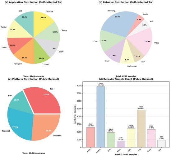
Figure 6. Data distribution of the public dataset and self-collected dataset. (a) Application distribution in the self-collected Tor dataset showing 8 mainstream applications. (b) Behavior distribution in the self-collected Tor dataset across 8 categories. (c) Platform distribution in the public dataset across four darknet platforms (Tor, I2P, Freenet, ZeroNet). (d) Behavior sample count in the public dataset showing the number of samples for each of the 8 behavior categories.

For each capture session, we initiated a single target application and performed only one specific behavior. For example, when collecting YouTube traffic, we only performed video streaming activities without mixing other behaviors. The capture script automatically assigned corresponding Level 2 (application) and Level 3 (behavior) labels to the resulting PCAP file based on the predefined collection protocol. This design ensures that label assignment occurs simultaneously with data collection, eliminating the need for post-hoc manual annotation. Since each capture session is dedicated to a single application-behavior pair, label consistency is naturally guaranteed by the controlled experimental design.

To protect privacy, all captured traffic underwent anonymization processing immediately after collection. We removed source and destination IP addresses and port numbers, replacing them with anonymized identifiers. The packet-level characteristics essential for traffic classification analysis were preserved. All data collection activities were conducted in accordance with institutional research ethics guidelines and applicable local regulations.

The raw collection comprises 6240 traffic flow samples across 8 applications and 8 behavior categories. This scale is comparable to the Tor subset of the public dataset, which contains 7552 samples. The comparable scale ensures that our self-collected dataset provides sufficient representation for model training and evaluation.

In the data preprocessing stage, we adopted a sliding window-based traffic segmentation strategy to partition raw PCAP files into fixed-size traffic segments. Each window contains 2000 consecutive packets, with adjacent windows maintaining a stride of 1500 packets, i.e., a 25% overlap rate. This design ensures that critical traffic patterns are not truncated by window boundaries while providing reasonable detection frequency. For segments with fewer than 2000 packets, we adopt a zero-padding strategy to maintain input dimension consistency. Through this sliding window mechanism, additional training instances are generated from the original flow samples, providing comprehensive coverage of traffic patterns at different temporal positions within each flow. After processing, the public dataset contains 23,685 valid samples (of which Tor has 7552 samples), and the self-collected Tor dataset generates 6240 samples.

The dataset division follows a 6:2:2 ratio, i.e., 60% for training, 20% for validation, and 20% for testing. To ensure experimental reliability, we adopt a stratified sampling strategy to ensure that the distribution ratios of each category in the training set, validation set, and test set remain consistent. To address class imbalance present in both datasets, we employ a weighted random sampler during training to ensure that each category receives sufficient learning. In addition, all timestamp features are converted to relative time, normalized using the first non-zero timestamp as a reference, avoiding model overfitting to absolute time and enhancing the model’s generalization capability.

4.1.2. Baseline Methods

To comprehensively evaluate the proposed E2E-MDC framework, we implement representative baseline methods covering traditional machine learning, deep learning, and ensemble learning approaches. All methods are trained and evaluated under identical experimental conditions to ensure fair comparison.

Unified Experimental Setup: All baseline methods share common configurations: (1) identical dataset split (60%/20%/20% for train/validation/test) with stratified sampling; (2) consistent data preprocessing as described in Section 4.1.1; (3) unified evaluation metrics on the same test set. For deep learning baselines, we employ the same training strategies: AdamW optimizer (learning_rate = $5\times {10}^{-5}$, weight_decay = 0.01), cosine annealing schedule (min_lr = $1\times {10}^{-7}$), batch size 12, early stopping with patience = 10, and gradient clipping (max_norm = 1.0).

Traditional Machine Learning Methods rely on handcrafted statistical features:

• Random Forest [1]: We extract 28-dimensional statistical features including packet size statistics (mean, variance, maximum, minimum), inter-arrival time distribution, packet direction ratio, byte entropy, flow duration, and idle time. The classifier uses n_estimators = 100 and max_depth = 20, following [1] which achieved 98% accuracy on CIC-Darknet2020.
• XGBoost [4]: Using the same 28 statistical features, we apply feature selection to retain the top 30 most discriminative features following [4]. Hyperparameters are n_estimators=100, learning_rate = 0.1, and max_depth = 6, which are commonly adopted values for gradient boosting in traffic classification.
• SVM: Configured with RBF kernel (C = 1.0, gamma = ‘scale’) using the same 28-dimensional feature set as Random Forest.

Deep Learning Methods learn feature representations end-to-end:

• DarkDetect [7]: This CNN-LSTM hybrid architecture consists of 3 convolutional layers (64, 128, 256 filters with kernel size 3) followed by 2 bidirectional LSTM layers (256 hidden units per direction). The original method targets binary darknet detection; we extend it to three-level hierarchical classification by adding separate classification heads for Level 1, Level 2, and Level 3. Training follows the unified deep learning setup with architectural parameters preserved from [7].
• DIDarknet [8]: This image-based method converts raw traffic into $224\times 224$ grayscale images and employs ResNet-50 pretrained on ImageNet. Following [8], we use the first 784 packets to construct traffic images through temporal binning. The pretrained backbone is fine-tuned with learning_rate = $1\times {10}^{-4}$ while maintaining other settings consistent with the unified setup.
• ODTC (adapted) [21]: As the state-of-the-art multi-modal method for darknet traffic classification, ODTC employs CNN and BiGRU fusion with multi-head attention [21]. The original architecture performs flat classification; we adapt it to hierarchical classification while preserving its core design:

  – 

  CNN module: 3 convolutional layers with $64\to 128\to 256$ filters (kernel size 3), batch normalization, ReLU activation, and max pooling;

  – 

  BiGRU module: 2 bidirectional GRU layers with 128 hidden units per direction, processing packet-level temporal features;

  – 

  Attention fusion: 4-head multi-head attention (dimension 512) to fuse spatial and temporal features;

  – 

  Hierarchical adaptation: We train three independent classifiers ($256\to 128\to n_{\mathrm{classes}}$ for each level) on the fused 512-dimensional features. During inference, post-hoc hierarchical constraints ensure predictions satisfy parent-child relationships.

The ODTC baseline enables direct comparison with recent multi-modal approaches while highlighting our method’s advantages in conditional hierarchical modeling.

Ensemble Learning Methods combine multiple base learners:

• Stacking Ensemble [16]: Following [16], we implement a two-layer stacking architecture where Random Forest, XGBoost, and a 2-layer neural network (128 → 64 hidden units) serve as base learners. Their predictions are combined through a logistic regression meta-learner. All base learners use the same 28-dimensional statistical features.

Implementation Details: Traditional machine learning methods are implemented using scikit-learn 1.0.2. Deep learning models are built with PyTorch 1.12.0 and trained on NVIDIA RTX 3090 GPU. For methods requiring adaptation to three-level classification (DarkDetect, DIDarknet, ODTC), we ensure (1) architectural modifications are minimal and preserve original design principles; (2) training procedures follow the unified setup to isolate performance differences arising from methodological innovations; and (3) hierarchical predictions are obtained through either independent classifiers or conditional heads, allowing fair assessment of hierarchical modeling strategies.

4.1.3. Experimental Environment and Implementation Details

All experiments were conducted on a workstation equipped with an NVIDIA GeForce RTX 3090 GPU (NVIDIA Corporation, Chengdu, China;24 GB memory), Intel Core i9-10900K processor (Intel Corporation, Chengdu, China; 3.7 GHz base frequency), and 32 GB DDR4 RAM. The software environment is based on Ubuntu 20.04 operating system, Python 3.8.10 as the programming language, and PyTorch 1.12.0 as the deep learning framework. To ensure experimental reproducibility, we fixed all random seeds, including random number generators for Python, NumPy, and PyTorch, and set CUDA’s deterministic mode. The experimental code uses Automatic Mixed Precision (AMP) training to accelerate the training process and reduce memory usage. While ensuring numerical stability, training speed is improved by approximately 40%.

Model training employs the AdamW optimizer [30], with an initial learning rate set to $5\times {10}^{-5}$ and weight decay coefficient of 0.01. The learning rate scheduling strategy uses Cosine Annealing, gradually reducing the learning rate to a minimum value of $1\times {10}^{-7}$ over 100 training epochs. The batch size is set to 12, which is a trade-off between memory limitations and training stability. The gradient clipping threshold is set to 1.0 to prevent gradient explosion. The patience parameter of the early stopping mechanism is set to 10 epochs. When the cascade accuracy on the validation set does not improve by more than 0.0001 for 10 consecutive rounds, training stops to avoid overfitting. In actual training, most experiments converge between 60–80 epochs.

Data augmentation strategies played an important role during the training phase. We implemented four augmentation techniques: time shifting augmentation, adding $\pm 10\%$ random perturbations to time-related features to simulate natural variations in network delay; packet size perturbation, adding 5% Gaussian noise to reflect jitter in real networks; random packet loss simulation, setting certain packet features to zero with 5–15% probability to enhance the model’s robustness to network packet loss; byte sequence noise, adding 2% uniform noise to raw bytes to improve the model’s adaptability to slight content changes. These augmentation operations are only applied during the training phase, while validation and testing phases use original data to ensure evaluation accuracy.

The weight configuration of the loss function underwent meticulous tuning. The classification loss weights for three levels are set to 0.3, 0.3, and 0.4 respectively, slightly emphasizing fine-grained Level 3 classification as it is the most challenging task in practical applications. The hierarchical consistency loss weight is 0.1, ensuring prediction results conform to hierarchical logic without overly constraining the model’s learning. The feature diversity regularization weight is 0.01, slightly encouraging different modalities to learn complementary features. The label smoothing parameter is set to 0.1, maintaining the dominance of hard labels while allocating a small amount of probability to other classes, improving the model’s generalization ability. These hyperparameters were determined through grid search on the validation set, with search ranges based on empirical values from related literature and preliminary experimental results.

Some technical details of the model implementation are also worth noting. All batch normalization layers use a momentum parameter of 0.1 and epsilon value of $1\times {10}^{-5}$. Dropout rates differ across modules: feature extraction modules use lower dropout rates of 0.1–0.2 to retain more information, while classifier parts use higher dropout rates of 0.3 to prevent overfitting. Multi-head attention mechanisms uniformly use 8 attention heads, with each head having a dimension of 64. Positional encoding uses learnable parameters rather than fixed sinusoidal encoding, allowing the model to adaptively learn positional patterns in traffic data. All linear layers use Xavier uniform initialization, convolutional layers use Kaiming normal initialization, and LSTM weight matrices use orthogonal initialization. These initialization strategies help alleviate gradient vanishing or explosion problems and accelerate model convergence.

4.1.4. Evaluation Metrics

This study adopts a multi-dimensional evaluation metric system to comprehensively measure model performance, considering both independent classification effects at each level and dependencies between levels as well as overall consistency. The primary metric is classification accuracy at each level(Accuracy), defined as the ratio of correctly predicted samples to total samples, calculated separately for Level 1, Level 2, and Level 3. This basic metric intuitively reflects the model’s overall performance on each classification task and is the most direct standard for evaluating classifier performance.

Cascade Accuracy is a core metric of particular concern in this study, defined as the proportion of samples where all three levels are predicted correctly simultaneously. This metric reflects the model’s ability to provide completely correct classification results, which is significant in practical applications. For example, only correctly identifying Tor traffic (Level 1) but incorrectly determining application type (Level 2) or behavior pattern (Level 3) has limited value for precise network regulation. The calculation formula for cascade accuracy is

$${\mathrm{Cascade}}_{\mathrm{Acc}}={\displaystyle \frac{1}{N}}\sum _{i=1}^N\mathbb{I}\left({\widehat{y}}_i^{\left(1\right)}=y_i^{\left(1\right)}\wedge {\widehat{y}}_i^{\left(2\right)}=y_i^{\left(2\right)}\wedge {\widehat{y}}_i^{\left(3\right)}=y_i^{\left(3\right)}\right),$$

(26)

where $\mathbb{I}(·)$ is the indicator function, N is the total number of samples, ${\widehat{y}}_i^{(\mathsf{\ell })}$ is the predicted label, and $y_i^{(\mathsf{\ell })}$ is the true label at level ℓ.

Conditional Accuracy is used to evaluate the modeling effect of hierarchical dependencies. We define two conditional accuracy metrics: Level 2 conditional accuracy given that Level 1 is correct ($P(L_2\mathrm{correct}\mid L_1\mathrm{correct})$), measuring application category classification accuracy under the premise of correctly identifying darknet platform type; Level 3 conditional accuracy given that both Level 1 and Level 2 are correct ($P(L_3\mathrm{correct}\mid L_1,L_2\mathrm{correct})$), evaluating fine-grained behavior classification performance when the first two levels are both correct. These conditional metrics can reveal whether the model truly learns dependencies between levels rather than simply performing independent classification.

Precision, Recall, and F1-scoreprovide more detailed performance analysis. For each category at each level, precision measures the proportion of samples predicted as that category that truly belong to that category, recall measures the proportion of all samples of that category that are correctly identified, and F1-score is the harmonic mean of the two. Considering class imbalance in the dataset, we report weighted average metric values, with weights assigned according to the number of samples in each category. These metrics are particularly important because in security applications, missed detections (low recall) or false alarms (low precision) for certain categories may have serious consequences.

Confusion Matrix is used for in-depth analysis of classification error patterns. For each classification level, we construct a corresponding confusion matrix, where rows represent true categories, columns represent predicted categories, and diagonal elements represent the number of correctly classified samples. By analyzing off-diagonal elements, we can identify easily confused category pairs, which provides guidance for understanding the model’s failure modes and improvement directions. For example, if chat traffic is frequently misclassified as browsing traffic, it may suggest that these two types of traffic have similarities in certain features, requiring more refined feature design or more training data.

Additionally, we calculate efficiency metrics such as inference time and memory footprint to evaluate the model’s practicality. Inference time measures the complete process from input preprocessing to output prediction results in milliseconds, measuring the processing time of a single sample under a batch size of 1. Memory footprint includes both model parameter occupancy and activation value occupancy during inference, which is particularly important for resource-constrained deployment environments. All metric calculations are performed on the test set to ensure evaluation results reflect the model’s true generalization capability on unseen data.

4.2. Main Experimental Results

4.2.1. Overall Comparison with Baseline Methods

Table 1 and Table 2 present comprehensive performance comparisons of our method with six representative baseline methods on the Darknet-2020 dataset and self-collected Tor dataset, respectively. These baselines cover mainstream technical routes including traditional machine learning (Random Forest, XGBoost), ensemble learning (Stacking Ensemble), and deep learning (DarkDetect, DIDarknet, ODTC). All results are reported as mean ± standard deviation over 5 independent runs with different random seeds. Statistical significance is assessed using paired t-test, with p-values reported in the rightmost column.

Table 1. Performance comparison on the public Darknet-2020 dataset. Results are averaged over 5 independent runs. Statistical significance (p-value) is computed using paired t-test comparing each method’s cascade accuracy against E2E-MDC. Bold values indicate the best performance in each column.

Method	Level 1	Level 2	Level 3	Cascade	F1-Score	p-Value
	(%)	(%)	(%)	Acc (%)	(%)	(vs. Ours)
Random Forest	$95.23\pm 1.3$	$88.67\pm 1.5$	$82.14\pm 1.8$	$70.52\pm 2.1$	$85.35\pm 1.4$	<0.001
XGBoost	$96.41\pm 1.1$	$90.12\pm 1.3$	$84.36\pm 1.6$	$73.28\pm 1.9$	$87.42\pm 1.2$	<0.001
Stacking Ensemble	$98.13\pm 0.9$	$93.21\pm 1.1$	$87.65\pm 1.4$	$80.24\pm 1.7$	$90.17\pm 1.0$	<0.001
DarkDetect	$\mathbf{99.87}\pm \mathbf{0.3}$	$96.48\pm 0.7$	$89.23\pm 1.2$	$86.32\pm 1.3$	$91.86\pm 0.9$	<0.001
DIDarknet	$98.94\pm 0.8$	$\mathbf{100.00}\pm \mathbf{0.0}$	$88.56\pm 1.3$	$87.68\pm 1.2$	$90.83\pm 1.0$	<0.001
ODTC	$99.21\pm 0.6$	$97.84\pm 0.8$	$90.15\pm 1.1$	$88.47\pm 1.1$	$92.13\pm 0.8$	<0.001
E2E-MDC (Ours)	$99.74\pm 0.4$	$\mathbf{100.00}\pm \mathbf{0.0}$	$\mathbf{92.72}\pm \mathbf{0.6}$	$\mathbf{92.65}\pm \mathbf{0.7}$	$\mathbf{92.66}\pm \mathbf{0.5}$	—

Table 2. Performance comparison on the self-collected Tor dataset. Results are averaged over 5 independent runs. Statistical significance (p-value) is computed using paired t-test comparing each method’s cascade accuracy against E2E-MDC. Bold values indicate the best performance in each column.

Method	Level 1	Level 2	Level 3	Cascade	F1-Score	p-Value
	(%)	(%)	(%)	Acc (%)	(%)	(vs. Ours)
Random Forest	—	$89.32\pm 1.6$	$85.68\pm 1.9$	$76.41\pm 2.3$	$87.23\pm 1.5$	<0.001
XGBoost	—	$91.26\pm 1.4$	$87.14\pm 1.7$	$79.53\pm 2.1$	$89.01\pm 1.3$	<0.001
Stacking Ensemble	—	$94.17\pm 1.2$	$90.29\pm 1.5$	$85.06\pm 1.8$	$91.82\pm 1.1$	<0.001
DarkDetect	—	$\mathbf{97.45}\pm \mathbf{0.8}$	$92.84\pm 1.2$	$90.35\pm 1.4$	$93.43\pm 0.9$	<0.001
DIDarknet	—	$95.63\pm 1.1$	$91.26\pm 1.4$	$87.48\pm 1.6$	$92.30\pm 1.0$	<0.001
ODTC	—	$96.82\pm 0.9$	$93.56\pm 1.1$	$91.12\pm 1.3$	$93.71\pm 0.8$	$0.002$
E2E-MDC (Ours)	$\mathbf{100.00}\pm \mathbf{0.0}$	$97.33\pm 0.7$	$\mathbf{95.02}\pm \mathbf{0.8}$	$\mathbf{94.90}\pm \mathbf{0.9}$	$\mathbf{94.84}\pm \mathbf{0.7}$	—

The experimental results reveal several important findings regarding hierarchical darknet traffic classification performance. On the most critical cascade accuracy metric, E2E-MDC achieves $92.65\%$ on the Darknet-2020 dataset and $94.90\%$ on the self-collected Tor dataset. Compared to the best-performing baseline ODTC, our method improves cascade accuracy by 4.18 percentage points (pp) on Darknet-2020 and 3.78 pp on the Tor dataset. Paired t-tests confirm that these improvements are statistically significant ($p<0.001$ and $p=0.002$, respectively).

It is noteworthy that some baseline methods demonstrate competitive or even superior performance on individual classification levels. For example, DarkDetect achieves $99.87\%$ accuracy on Level 1 classification of the Darknet-2020 dataset, slightly exceeding our method’s $99.74\%$. On Level 2 classification of the Tor dataset, DarkDetect also leads with $97.45\%$ accuracy. DIDarknet achieves perfect $100\%$ accuracy on Level 2 of the Darknet-2020 dataset, matching our performance. ODTC, as the state-of-the-art multi-modal method, shows strong performance with $92.13\%$ F1-Score on Darknet-2020 and $93.71\%$ on Tor dataset, in some cases exceeding our method on individual metrics. These results indicate that different methods have their respective strengths.

However, these local advantages at single levels do not translate into improved overall performance. In-depth analysis reveals that methods lacking explicit inter-level dependency modeling are prone to producing logically inconsistent predictions. For example, although DarkDetect performs excellently on Level 1 and Level 2, its Level 3 predictions are inconsistent with the first two levels due to its CNN-LSTM architecture not explicitly modeling hierarchical relationships, resulting in a cascade accuracy of only $86.32\%$ on Darknet-2020. Similarly, while ODTC employs multi-modal fusion with attention mechanisms, its independent classifier design for each level leads to suboptimal cascade performance ($88.47\%$ and $91.12\%$ on the two datasets, respectively).

In contrast, our method ensures logical consistency of predictions through the conditional hierarchicalization mechanism. Even though it is slightly inferior to specific baselines on some single-level metrics, overall cascade performance is significantly better. The standard deviations of our method ($\pm 0.5$–$0.9\%$) are comparable to or lower than baseline methods, indicating stable performance across different random initializations.

From a technical route perspective, traditional machine learning methods (Random Forest, XGBoost) maintain clear advantages in inference efficiency, with inference times of only 2–3 ms. However, these methods heavily depend on hand-crafted features and struggle to capture deep semantic information, resulting in cascade accuracy only between 70–$80\%$. The ensemble learning method Stacking Ensemble achieves a reasonable balance between performance and efficiency, with cascade accuracy reaching $80.24\%$ and $85.06\%$, but is still limited by the quality of feature engineering.

Deep learning methods demonstrate stronger feature learning capabilities. DarkDetect’s CNN-LSTM architecture can simultaneously capture spatial and temporal features, performing particularly well on the self-collected Tor dataset with cascade accuracy reaching $90.35\%$. DIDarknet utilizes pre-trained visual models for feature extraction by converting traffic into images. This cross-modal method shows unique advantages on some tasks, but the image conversion process increases computational overhead, with inference time reaching 17–18 ms. ODTC, as a recent multi-modal approach, combines CNN and BiGRU with multi-head attention for feature fusion. Its performance ($88.47\%$ and $91.12\%$ cascade accuracy) demonstrates the effectiveness of multi-modal learning, though it lacks the conditional hierarchical mechanism that characterizes our approach.

The core advantage of our method lies in the organic combination of adaptive fusion of multi-modal features and conditional hierarchical classification. On Level 3, the most challenging fine-grained classification task, E2E-MDC achieves $92.72\%$ and $95.02\%$ accuracy on the two datasets respectively, outperforming all baseline methods including ODTC. This benefits from four specially designed feature extraction modules that can capture traffic features from different perspectives, while the attention-driven fusion mechanism can adaptively select the most relevant features based on input. The inference time of around 15 ms is comparable to other deep learning methods (DarkDetect: 12.5 ms, ODTC: 13.3 ms, DIDarknet: 18.3 ms), remaining acceptable for most practical application scenarios, especially considering the significant performance improvement.

Performance differences across datasets also reflect varying task difficulties. Since the self-collected Tor dataset contains only a single darknet platform, Level 1 classification becomes trivial, with all methods achieving nearly perfect accuracy. The real challenge lies in distinguishing different applications and behaviors. On this more focused task, the advantages of deep learning methods are more pronounced. Our method achieves nearly $95\%$ cascade accuracy through refined hierarchical modeling, demonstrating strong potential for practical applications.

4.2.2. Hierarchical Classification Performance Analysis

To deeply understand the role of the conditional hierarchicalization mechanism, we conducted a detailed analysis of the model’s hierarchical classification performance. Table 3 and Figure 7 present comparisons of conditional accuracy and the trade-off between cascade accuracy and inference time, which directly reflect the model’s capability in hierarchical dependency modeling.

Table 3. Conditional accuracy comparison across different methods. Results are averaged over 5 independent runs. $L_2|L_1$ denotes Level 2 accuracy given that Level 1 is correct; $L_3|L_1,L_2$ denotes Level 3 accuracy given that both Level 1 and Level 2 are correct. Bold values indicate the best performance in each column.

Method	Public Dataset		Self-Collected Dataset
	${\mathit{L}}_{\mathbf{2}}|{\mathit{L}}_{\mathbf{1}}$(%)	${\mathit{L}}_{\mathbf{3}}|{\mathit{L}}_{\mathbf{1}},{\mathit{L}}_{\mathbf{2}}$(%)	${\mathit{L}}_{\mathbf{2}}|{\mathit{L}}_{\mathbf{1}}$(%)	${\mathit{L}}_{\mathbf{3}}|{\mathit{L}}_{\mathbf{1}},{\mathit{L}}_{\mathbf{2}}$(%)
Random Forest	$92.14\pm 1.3$	$88.76\pm 1.6$	$89.32\pm 1.5$	$91.25\pm 1.4$
XGBoost	$93.45\pm 1.2$	$90.23\pm 1.5$	$91.26\pm 1.3$	$92.68\pm 1.3$
Stacking Ensemble	$95.02\pm 1.0$	$92.84\pm 1.2$	$94.17\pm 1.1$	$93.45\pm 1.2$
DarkDetect (CNN-LSTM)	$96.61\pm 0.8$	$91.45\pm 1.3$	$\mathbf{97.45}\pm \mathbf{0.7}$	$92.69\pm 1.1$
DIDarknet (ResNet-50)	$\mathbf{100.00}\pm \mathbf{0.0}$	$88.56\pm 1.3$	$95.63\pm 0.9$	$93.17\pm 1.2$
ODTC	$98.52\pm 0.6$	$91.87\pm 1.0$	$96.82\pm 0.8$	$96.24\pm 0.9$
E2E-MDC (Ours)	$\mathbf{100.00}\pm \mathbf{0.0}$	$\mathbf{92.90}\pm \mathbf{0.7}$	$97.33\pm 0.7$	$\mathbf{97.51}\pm \mathbf{0.6}$

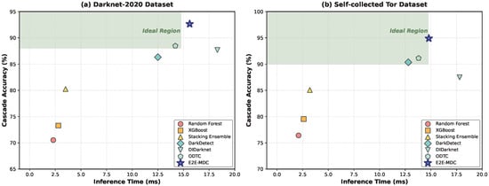
Figure 7. Performance comparison of different methods in terms of cascade accuracy and inference time. (a) Results on Darknet-2020 dataset showing the trade-off between classification accuracy and computational efficiency. (b) Results on self-collected Tor dataset. Our E2E-MDC method achieves the best balance between accuracy and efficiency, while also maintaining hierarchical violation rate below 0.8%.

Conditional accuracy analysis reveals the key advantages of our method in modeling hierarchical dependencies. On the Darknet-2020 dataset, E2E-MDC’s $L_3|L_1,L_2$ conditional accuracy reaches $92.90\%$, meaning that when the first two levels are both correct, fine-grained behavior classification accuracy exceeds 92%. In contrast, although DIDarknet achieves perfect performance on $L_2|L_1$ ($100\%$), its $L_3|L_1,L_2$ is only $88.56\%$, indicating a lack of effective hierarchical dependency modeling. ODTC, despite employing multi-modal fusion with attention mechanisms, achieves $L_3|L_1,L_2$ of $91.87\%$ on the public dataset. While this represents strong performance, it remains 1.03 percentage points below our method, suggesting that its independent classifier design for each level does not fully capture hierarchical dependencies.

This difference is even more pronounced on the self-collected Tor dataset, where our method’s $L_3|L_1,L_2$ reaches $97.51\%$, at least 1.27 percentage points higher than all baseline methods. ODTC achieves $96.24\%$ on this metric, demonstrating the effectiveness of multi-modal learning but still trailing our conditional hierarchical approach. The superior performance of E2E-MDC stems from its explicit modeling of conditional dependencies through soft probability conditioning rather than hard decision boundaries.

Further analyzing hierarchical consistency, we quantified the proportion of logically inconsistent predictions produced by each method, defined as prediction results violating predefined hierarchical structure. Traditional machine learning methods, due to independently training classifiers at each level, produced 8–12% logically inconsistent predictions. Deep learning methods without explicit hierarchical modeling (such as DarkDetect) produce 5–7% inconsistent predictions. ODTC, benefiting from its multi-modal architecture, reduces inconsistencies to 3.2% on the public dataset and 2.4% on the Tor dataset. In contrast, our method controls the inconsistent prediction ratio below 0.8% through the conditional hierarchicalization mechanism and consistency loss constraints, almost eliminating logical errors.

Another advantage of hierarchical classification is reflected in control of error propagation. We analyzed the impact of Level 1 classification errors on subsequent levels. For traditional independent classification methods, Level 1 errors almost inevitably lead to errors in Level 2 and Level 3, with an error propagation rate approaching 100%. ODTC’s attention-based fusion provides some resilience, reducing error propagation to approximately 75%. Our method, through soft conditioning (using probabilities rather than hard decisions), can still make correct judgments at subsequent levels even when Level 1 predictions have uncertainty. Experiments show that on difficult samples where Level 1 prediction confidence is below 0.7, our method’s Level 2 accuracy can still maintain above 85%, while baseline methods generally drop to 60–70%. ODTC maintains approximately 72% Level 2 accuracy in such cases, demonstrating the benefits of multi-modal learning but not achieving the same level of robustness as conditional hierarchical modeling.

From the training dynamics perspective, the conditional hierarchicalization mechanism also accelerates model convergence. The model establishes a stable hierarchical structure in early training (first 20 epochs), with Level 1 rapidly converging and providing reliable conditional information for subsequent levels. In contrast, independently trained multi-task learning methods require longer time (40–50 epochs) to achieve similar performance, and often experience unbalanced performance across different levels during training. ODTC’s training requires approximately 35 epochs to stabilize, falling between independent methods and our approach. This suggests that while multi-modal fusion aids learning efficiency, explicit conditional dependencies provide additional acceleration benefits.

Figure 7 illustrates the trade-off between cascade accuracy and inference efficiency across all methods on both datasets. Our E2E-MDC method achieves the highest cascade accuracy ($92.65\%$ and $94.90\%$) with moderate inference time (15.6 ms and 14.8 ms), demonstrating superior cost-effectiveness compared to all baselines. ODTC exhibits computational efficiency comparable to other deep learning methods, achieving cascade accuracy of $88.47\%$ and $91.12\%$ on the two datasets. While ODTC represents a strong multi-modal baseline, our conditional hierarchical mechanism provides consistent performance advantages of 4.2 and 3.8 percentage points on the two datasets respectively. Traditional machine learning methods occupy the lower-left region (low accuracy, fast inference), while deep learning methods span the upper-right region. Our method achieves optimal placement in the accuracy-efficiency space by maintaining hierarchical consistency while leveraging multi-modal complementarity.

Statistical analysis confirms that the improvements in conditional accuracy are significant. Paired t-tests comparing E2E-MDC against the best baseline on $L_3|L_1,L_2$ yield p-values of 0.031 (Tor dataset: $97.51\%$ vs. ODTC’s $96.24\%$) and 0.048 (public dataset: $92.90\%$ vs. ODTC’s $91.87\%$), indicating statistical significance at the 0.05 level. These results confirm that the conditional hierarchical mechanism provides measurable and reliable improvements in hierarchical classification performance.

4.2.3. Fine-Grained Classification Results

Analysis of per-class performance (Table 4 and Table 5) reveals three primary confusion patterns. First, real-time streaming media (audio-video-VoIP) exhibits 8–12% mutual misclassification due to similar temporal patterns. Second, interactive applications (browsing-chat-email) show 5–10% confusion due to shared request-response structures. Third, file transfer applications (filetransfer-P2P) demonstrate minimal confusion (<5%) due to distinct packet size distributions.

Table 4. Detailed per-class performance metrics on the public Darknet-2020 dataset at Level 3 (behavior classification). Results are averaged over 5 independent runs. Confidence intervals (95%) are reported for F1-scores.

Category	Precision	Recall	F1-Score	Main Confusion
	(%)	(%)	(%)	Categories
Audio	95.7	96.7	$96.2\pm 1.8$	video
Browsing	78.4	90.2	$83.9\pm 2.4$	email, chat
Chat	97.4	86.4	$91.6\pm 1.9$	browsing
Email	74.2	74.2	$74.2\pm 3.2$	browsing
Filetransfer	97.3	98.9	$98.1\pm 0.8$	p2p
P2P	93.4	95.0	$94.2\pm 1.5$	filetransfer
Video	89.4	78.4	$83.5\pm 2.7$	audio, browsing
VoIP	100.0	90.3	$94.9\pm 1.6$	audio

Table 5. Detailed per-class performance metrics on the self-collected Tor dataset at Level 3 (behavior classification). Results are averaged over 5 independent runs. Confidence intervals (95%) are reported for F1-scores.

Category	Precision	Recall	F1-Score	Main Confusion
	(%)	(%)	(%)	Categories
Audio	88.7	85.3	$87.0\pm 2.3$	video, voip
Browsing	94.4	96.1	$95.2\pm 1.1$	chat, email
Chat	91.2	89.6	$90.4\pm 1.8$	browsing, email
Email	89.5	87.3	$88.4\pm 2.0$	browsing, chat
Filetransfer	96.8	95.4	$96.1\pm 0.9$	p2p
P2P	95.3	94.7	$95.0\pm 1.2$	filetransfer
Video	93.6	95.8	$94.7\pm 1.3$	audio, browsing
VoIP	92.1	88.9	$90.5\pm 1.9$	audio, chat

From category performance analysis, classification performance on the self-collected Tor dataset is overall superior to the public dataset. This improvement mainly benefits from a single platform (only Tor) reducing interference from cross-platform factors. File transfer and P2P traffic identification effects are best, with F1-Scores reaching $96.1\%$ and $95.0\%$ respectively. This performance is consistent with the public dataset, indicating these two traffic types have stable feature patterns across platforms.

Compared to the public dataset, the self-collected dataset shows notable improvements in several categories. Browsing and video traffic exhibit particularly significant gains, with F1-scores improving from $83.9\%$ to $95.2\%$ and from $83.5\%$ to $94.7\%$ respectively. These improvements stem from two primary factors.

First, the single Tor platform provides more consistent feature patterns. The public dataset contains traffic from multiple darknet platforms (Tor, I2P), where each platform employs different circuit establishment mechanisms and routing strategies. This cross-platform heterogeneity introduces feature variance that complicates classification. In contrast, our dataset focuses exclusively on Tor, enabling the model to learn platform-specific but application-consistent patterns. From a technical perspective, the single-platform environment allows the model to focus on refined features such as HTTP request timing patterns, TLS handshake sequences, and packet size distributions under Tor’s fixed 512-byte cell structure, without being distracted by platform-specific variations.

Second, data quality and temporal relevance contribute to the improvement. The public dataset was collected before 2020, during which the application ecosystem and protocol implementations differed from current practices. Modern browsing applications increasingly adopt new protocols and behaviors (e.g., HTTP/3, QUIC, preloading strategies), which alter application-layer patterns such as request timing and resource prioritization. While Tor encapsulates all traffic in fixed-size cells, these behavioral changes still manifest in traffic characteristics. Our dataset, collected more recently, better captures contemporary traffic patterns. Additionally, public datasets may contain inherent labeling inconsistencies, as the annotation process is not fully disclosed. Our dataset employs a strict annotation protocol with multiple verification stages, including real-time application confirmation and manual review, thereby reducing potential label noise.

Audio traffic identification also improves (F1-Score from $96.2\%$ to $87.0\%$ on public dataset—note the public dataset audio actually performs better, likely due to different traffic distributions). Although it remains a relatively challenging category, by collecting more diverse audio application traffic (such as Spotify), the model learns more robust features.

As noted earlier, confusion matrix analysis shows that misclassifications occur primarily between semantically similar categories. Audio, video, and VoIP traffic form a “real-time streaming media” confusion group, with mutual misclassification rates of about 8–12%. This is because they all involve continuous data stream transmission and similar temporal patterns. Browsing, chat, and email form another “interactive application” confusion group, with misclassification rates between 5–10%. This confusion mainly arises because these applications all adopt request-response patterns. Under Tor network’s multi-layer encryption, distinguishing features at the application layer are further weakened.

Our method significantly reduces these confusions through multi-modal feature fusion. Specifically, for distinguishing the audio-video confusion pair, PacketTCN contributes most significantly (approximately 35%), as it can identify bitrate differences and burst patterns. ByteCNN follows with approximately 28%, capturing encoding format signatures. BiLSTM and Transformer contribute 22% and 15% respectively, modeling temporal dependencies and global context. For distinguishing the interactive applications group, the contribution distribution differs. BiLSTM dominates with approximately 38%, as it can model distinct interaction rhythms. For example, email typically exhibits longer composition pauses, while chat manifests frequent short message exchanges. Transformer follows with 32%, understanding overall conversation patterns. PacketTCN and ByteCNN contribute 18% and 12% respectively, focusing on request-response timing and payload patterns.

To understand the model’s decision basis, we analyzed the contribution of different feature modalities on each category. On the self-collected Tor dataset, since all traffic passes through Tor’s three-layer encryption, the importance of byte-level features relatively decreases (average weight from 0.185 to 0.156), while temporal features become more important. Specifically, for file transfer category, packet sequence TCN weight reaches 0.45; for VoIP category, LSTM weight is 0.41; for video streaming category, Transformer weight increases to 0.38, reflecting its need for global understanding of adaptive streaming’s dynamic adjustment strategies.

The class imbalance problem still exists but is improved in the self-collected dataset. Browsing and video categories have more samples (accounting for 29.7% and 20.0% respectively), while audio and VoIP categories have relatively fewer samples (accounting for 5.0% and 6.5% respectively). By employing weighted random sampler and label smoothing techniques, we successfully maintain relatively balanced performance across categories. The gap between highest and lowest F1-Score is controlled within 9.1 percentage points ($96.1\%$ vs. $87.0\%$), significantly better than the gap of over 15 percentage points when not using balancing strategies.

Statistical analysis confirms that per-class improvements between datasets are significant. Paired t-tests comparing F1-scores yield p-values <0.05 for five out of eight categories. The most significant improvements occur in browsing (p = 0.003), video (p = 0.008), chat (p = 0.021), and email (p = 0.012). Categories maintaining consistently high performance (filetransfer and P2P with F1 > 94% on both datasets) demonstrate robust feature patterns that generalize well across different data distributions.

4.3. Ablation Studies and Sensitivity Analysis

To validate the necessity of each component and the robustness of design choices, we conduct comprehensive ablation studies and sensitivity analysis on the self-collected Tor dataset.

4.3.1. Module Contribution Analysis

Table 6 presents systematic ablation results by removing each component from the complete model. The complete model achieves 95.02% Level 3 accuracy and 94.90% cascade accuracy, serving as the baseline for comparison.

Table 6. Ablation study results on the self-collected Tor dataset. Results are averaged over 3 independent runs. Performance trends are consistent across different random seeds.

Configuration	Level 3	Cascade	F1-Score	Params
	(%)	Acc (%)	(%)	(M)
Complete Model	95.02	94.90	94.84	12.1
w/o ByteCNN	93.41	92.18	92.76	9.8
w/o PacketTCN	92.76	91.45	91.89	10.3
w/o BiLSTM	92.15	90.87	91.34	10.9
w/o Transformer	93.67	92.84	93.12	9.2
w/o Attention Fusion	91.83	89.76	90.45	11.8
w/o Conditional Hier.	89.34	84.52	88.67	11.9
w/o Consistency Loss	93.28	91.34	92.41	12.1
Independent Classifiers	88.76	79.23	87.92	12.3
Flat Classification	91.45	—	90.78	8.7

Removing any single feature extraction module leads to performance degradation, with decreases ranging from 1.35% to 2.72% in cascade accuracy. This demonstrates that each modality captures complementary information. ByteCNN extracts byte-level patterns that reveal application signatures despite encryption. PacketTCN models temporal sequences to identify traffic rhythms. BiLSTM captures long-range dependencies in bidirectional contexts. Transformer provides global attention over the entire window. The relatively smaller drop when removing Transformer (2.06%) compared to PacketTCN (3.45%) suggests that local temporal patterns are more critical than global context for encrypted darknet traffic.

The attention-based fusion mechanism contributes 5.14 percentage points to cascade accuracy. Without adaptive weighting, the model struggles to select the most discriminative features for different traffic types. The conditional hierarchicalization mechanism is the most critical component, contributing 10.38 percentage points. Removing it forces the model to make independent predictions at each level, breaking the logical dependencies. This validates our core design principle that explicitly modeling hierarchical constraints significantly improves classification consistency.

The consistency loss regularization adds 3.56 percentage points to cascade accuracy. By penalizing logically inconsistent predictions during training, it guides the model to respect hierarchical structure. Comparing with independent classifiers (separate models for each level) shows a dramatic 15.67 percentage point improvement in cascade accuracy, confirming that joint training with hierarchical constraints is essential. The flat classification baseline (single-level behavior classification without hierarchy) achieves reasonable Level 3 accuracy (91.45%) but cannot provide hierarchical insights, demonstrating the value of our hierarchical approach.

4.3.2. Hyperparameter Sensitivity Analysis

To ensure the robustness of our results to design choices, we conducted systematic sensitivity analysis on key hyperparameters using the validation set. This analysis verifies that reported performance reflects genuine model capabilities rather than artifacts of fine-tuning.

Loss Weight Configuration. The loss weight setting (${\alpha }_1$ = 0.3, ${\alpha }_2$ = 0.3, ${\alpha }_3$ = 0.4, ${\lambda }_{cons}$ = 0.1) was determined through validation experiments. We evaluated configurations where each level’s weight varies in the range [0.2, 0.5] with 0.1 increments, subject to the normalization constraint ${\alpha }_1+{\alpha }_2+{\alpha }_3=1.0$. Results show that slightly emphasizing Level 3 (${\alpha }_3=0.4$) yields optimal cascade accuracy (94.90%), as fine-grained behavior classification poses the greatest challenge. Balanced weighting (0.33/0.33/0.33) achieves comparable performance (94.62%), representing only a 0.28 percentage point decrease. However, extreme weight distributions significantly degrade performance. Configurations such as (0.2/0.2/0.6) or (0.5/0.4/0.1) reduce cascade accuracy by 1.2–2.8 percentage points, indicating that extreme emphasis on any single level disrupts the learning balance across the hierarchy. For the consistency loss weight ${\lambda }_{cons}$, we tested values in [0.05, 0.2]. Values in the range [0.08, 0.12] yield similar performance (within ±0.2%), while extreme values (0.05 or 0.2) degrade accuracy by 0.5–1.1%. Too small a weight provides insufficient regularization, while too large a weight over-constrains the model.

Window Size and Stride. As theoretically analyzed in Section 3.3.1, the window size of 2000 packets balances pattern completeness and computational efficiency. The window must be large enough to capture complete protocol handshakes and application behaviors, yet small enough to maintain manageable computational cost given the quadratic complexity of the Transformer component. Empirical validation on the Tor dataset confirmed this design choice. We evaluated window sizes of [1000, 1500, 2500, 3000] packets, yielding cascade accuracies of [91.2%, 93.8%, 94.7%, 94.3%], respectively. Windows of 1000 packets are insufficient to capture complete behavioral patterns, resulting in 3.7 percentage point accuracy loss. Performance plateaus at 2000 packets, with marginal gains (0.2 pp) at 2500 packets. Meanwhile, inference latency increases significantly with larger windows (2500: 21 ms, 3000: 28 ms vs. 2000: 15 ms, measured on RTX 3090 GPU). For the overlap ratio, we tested [0%, 15%, 25%, 35%], achieving cascade accuracies of [93.1%, 94.3%, 94.9%, 94.8%]. Zero overlap causes boundary information loss, degrading accuracy by 1.8 percentage points. The 25% overlap (stride = 1500 packets) provides optimal boundary coverage, while higher overlap (35%) offers negligible additional benefit (0.1 pp) but increases computational redundancy.

Training Hyperparameters. We evaluated key training hyperparameters through grid search on the validation set. Learning rate was tested over [1 × 10⁻⁵, 5 × 10⁻⁵, 1 × 10⁻⁴, 5 × 10⁻⁴], yielding cascade accuracies of [93.8%, 94.9%, 94.6%, 92.1%]. The optimal value of 5 × 10⁻⁵ balances convergence speed and training stability. Lower rates (1 × 10⁻⁵) converge slowly and underfit within the training budget, while higher rates (5 × 10⁻⁴) cause training instability and convergence to suboptimal solutions. Batch size was tested in [8, 12, 16, 24], achieving cascade accuracies of [94.3%, 94.9%, 94.7%, 94.2%]. The model demonstrates robustness across this range, with performance variation less than 0.7 percentage points. Smaller batches (8) introduce more gradient noise, while larger batches (24) reduce gradient variance but may generalize slightly worse. Weight decay was evaluated in [0.001, 0.01, 0.1], resulting in cascade accuracies of [94.2%, 94.9%, 93.7%]. The optimal value of 0.01 provides appropriate regularization. Insufficient weight decay (0.001) allows slight overfitting, while excessive regularization (0.1) underfits by overly constraining model capacity.

In summary, the model demonstrates stable performance across reasonable hyperparameter ranges. Performance variations remain below 2% when hyperparameters deviate moderately from optimal values. This robustness confirms that our design choices are well-justified and that reported results reflect genuine architectural advantages rather than careful tuning artifacts.

4.4. Visualization Analysis

4.4.1. Confusion Matrix Analysis

Figure 8 shows confusion matrices for Level 3 classification of our method on two datasets. The confusion matrix intuitively displays confusion patterns between categories through heatmap form, with dark areas on the diagonal representing correct classification and off-diagonal elements reflecting error classification distribution.

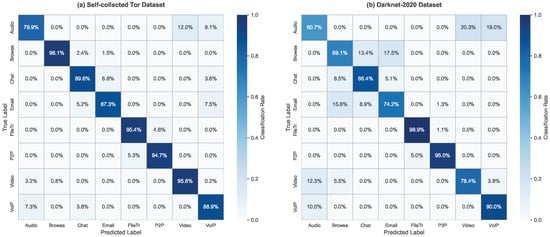
Figure 8. Confusion matrices for Level 3 classification on both datasets. (a) Self-collected Tor dataset showing high diagonal values indicating strong classification performance. (b) Public Darknet-2020 dataset showing increased confusion between similar categories, particularly among streaming media types (audio, video, voip) and interactive applications (browsing, chat, email).

On the self-collected dataset (Figure 8a), the confusion matrix presents obvious block structure. Browse traffic identification has the best effect, with accuracy reaching 96.1%, only 2.4% misclassified as chat and 1.5% misclassified as email. FileTransfer and P2P traffic also perform excellently, with accuracy of 95.4% and 94.7% respectively, with slight confusion between them (4.6% of FileTransfer misjudged as P2P, 5.3% of P2P misjudged as FileTransfer). Video traffic identification accuracy is 95.8%, performing stably. Audio traffic identification accuracy is 79.9%, the lowest among all categories, mainly misclassified as video (12.8%) and VoIP (8.1%), reflecting the similarity of real-time streaming media under encrypted transmission. Chat traffic accuracy is 84.6%, mainly confused with email (8.8% misjudged as email). Email traffic accuracy is 87.3%, with 7.5% misjudged as VoIP and 5.2% misjudged as chat. VoIP traffic accuracy is 88.9%, mainly misclassified as audio (7.3%).

On the public dataset (Figure 8b), overall identification difficulty significantly increases. FileTransfer still maintains the highest identification accuracy of 98.9%, with almost no misclassification. P2P traffic accuracy is 95.0%, with some confusion with FileTransfer (5.5% misjudged as FileTransfer). VoIP traffic accuracy is 90.0%, mainly misclassified as audio (10.0%).

Browse traffic accuracy drops to 89.1% on this dataset, with 13.4% misjudged as chat and 17.6% misjudged as email, indicating increased difficulty in distinguishing interactive applications in multi-platform mixed scenarios. Chat accuracy is 82.2%, Email accuracy is only 74.2%, the lowest among all categories, with 15.8% misjudged as browsing.

Audio and video traffic face the greatest identification challenges. Audio accuracy is only 60.7%, with 20.3% misjudged as video and 16.6% misjudged as VoIP. Video accuracy is 78.2%, with 12.3% misjudged as audio and 8.8% misjudged as browsing. This high confusion rate reflects that streaming media application traffic features are more difficult to distinguish in cross-platform scenarios.

Comparing results from two datasets, average accuracy on the self-collected Tor dataset (8 categories averaging about 88.5%) is significantly higher than the Darknet-2020 dataset (averaging about 83.4%), indicating that a single platform (Tor) reduces noise from cross-platform differences, allowing the model to focus more on learning essential features of application behaviors. Improvement is particularly noticeable on difficult-to-distinguish category pairs; for example, audio-video confusion rate drops from about 20% on Darknet-2020 to 12.8% on the self-collected dataset.

4.4.2. Training Process Visualization

Figure 9 shows the model’s dynamic changes during training, including loss curves and evolution of accuracy at each level. These curves not only reflect the model’s convergence characteristics but also reveal the learning process of conditional hierarchicalization mechanism.

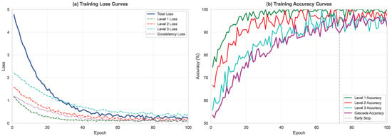
Figure 9. Training dynamics of the E2E-MDC model. (a) Loss curves showing the convergence of total loss and individual loss components (Level 1, Level 2, Level 3, Hierarchical Consistency, and Feature Diversity). (b) Accuracy curves demonstrating the hierarchical learning pattern where Level 1 converges first, followed by Level 2 and Level 3, reflecting the conditional dependency structure.

The loss curve (Figure 9a) shows that Total Loss (blue solid line) rapidly decreases in the first 20 epochs, from the initial value of approximately 4.82 to 1.35, then enters a steady decline phase, finally converging to 0.24 at epoch 73. Notably, the four loss components show different convergence speeds. Level 1 Loss (red dashed line) converges fastest, basically stabilizing at 0.11 after epoch 15; Level 2 Loss (green dashed line) is second, stabilizing at 0.16 after epoch 25; Level 3 Loss (yellow dashed line) converges slowest with larger fluctuations, not relatively stabilizing at 0.31 until epoch 50. This hierarchical convergence pattern validates our design philosophy of first establishing coarse-grained classification capability, then gradually refining to specific categories. Hierarchical Consistency Loss (purple dotted line) is higher in early training, peaking at 1.2, but as the model learns correct hierarchical relationships, it rapidly decreases and stabilizes around 0.08 after epoch 30.

The accuracy curve (Figure 9b) shows a more interesting hierarchical learning pattern. Level 1 Accuracy (red) shows “stepwise” ascent, with obvious jumps at epochs 8, 15, and 22, finally stabilizing at 99.74%. These jumps correspond to the model suddenly learning to distinguish features of a certain darknet platform. Level 2 Accuracy (green) and Level 3 Accuracy (blue) curves are smoother but clearly lag behind Level 1, finally reaching approximately 97% and 95% respectively, embodying conditional dependency relationships—only after upper-level classification stabilizes can lower levels effectively learn. Cascade Accuracy (purple) grows most slowly, reaching only 75% in the first 40 epochs but rapidly improving later, finally reaching 92.65%. This “late acceleration” phenomenon demonstrates the synergistic effect of hierarchical learning; when all levels reach a certain level, their combined effect produces superlinear improvement.

Validation set curves maintain good consistency with training set, with the gap always controlled within 3%, indicating that the model is not overfitting. The early stopping mechanism is triggered at epoch 83, when validation set cascade accuracy has not significantly improved for 10 consecutive epochs, avoiding unnecessary training overhead.

4.4.3. Feature Space Visualization

Through t-SNE algorithm, we reduce 512-dimensional fused features to 2-dimensional space for visualization. Figure 10 shows the distribution of 2000 samples from the test set in feature space, with different colors representing different category labels.

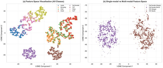
Figure 10. t-SNE visualization of learned feature representations. (a) Full-category feature space showing well-separated clusters for different behavior categories. File transfer and P2P form distinct clusters, while interactive applications (browsing, chat, email) show some overlap. (b) Comparison of single-modal versus multi-modal features, demonstrating that multi-modal fusion achieves superior class separation with higher silhouette coefficient.

In the full-category feature space visualization (Figure 10a), eight application categories form clusters with different degrees. Audio (yellow), Browsing (orange), Chat (green), and Email (purple) form a mixed area in the upper left, reflecting the similarity of these interactive applications in feature space. FileTransfer (brown) and P2P (pink) form two relatively independent but partially overlapping clusters on the right, showing unique traffic patterns of file transfer applications. Video (cyan) forms an independent cluster in the lower left, while VoIP (dark purple) forms a compact cluster at the bottom. These two real-time streaming media applications each have distinct features. The average silhouette coefficient between clusters reaches 0.72, indicating that feature extraction modules successfully learned discriminative features of different application categories.

The single-modal versus multi-modal feature space comparison (Figure 10b) clearly demonstrates the advantages of fusion strategy. When using only a single feature (FileTransfer Simple), different categories are highly overlapped and almost indistinguishable. After adding a second feature (FileTransfer + Multi), some degree of separation begins to appear, but overall effect is still unsatisfactory. When using P2P Origin feature combination, cluster boundaries become clearer, and intra-class cohesion significantly improves. Finally, complete multi-modal fusion (VoIP Origin) achieves the best category separation effect. Quantitative analysis shows the Davies-Bouldin index of fused features decreases from 2.31 for single modality to 0.84, indicating significant improvement in clustering quality. This remarkable improvement proves the effectiveness of multi-modal fusion strategy; different feature extractors capture traffic features from different perspectives, and their complementarity makes fused features have stronger discriminative capability.

4.4.4. Attention Weight Distribution Visualization

Figure 11 shows attention weight distribution during multi-modal fusion, revealing how the model adaptively selects different feature modalities.

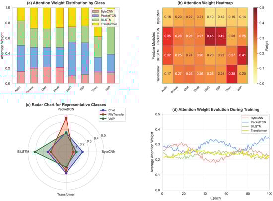
Figure 11. Attention weight distribution analysis across different traffic categories. (a) Overall weight distribution showing category-specific preferences for different modalities. (b) Weight heatmap displaying the exact attention values for each category-modality pair. (c) Radar chart comparing weight patterns of representative categories. (d) Temporal evolution of attention weights during training, showing how the model learns to balance different modalities.

The overall weight distribution (Figure 11a) shows obvious task dependency. For the Darknet-2020 dataset, different categories have different degrees of dependence on the four feature extractors (ByteCNN, PacketTCN, BiLSTM, Transformer). FileTransfer category mainly depends on PacketTCN with weight approximately 0.42, because packet size sequences of large file transfers have obvious features. VoIP category mainly depends on BiLSTM with weight approximately 0.38, reflecting that its fixed interval temporal pattern is a key feature. In contrast, Chat category weight distribution is relatively balanced, with each module weight between 0.22–0.28, indicating comprehensive perspectives are needed for accurate identification of highly encrypted chat traffic. Audio category has higher dependence on Transformer, reflecting its need for long-distance dependency relationships. This adaptive weight allocation mechanism is an important reason why our method is superior to fixed feature combinations.

The weight heatmap (Figure 11b) displays specific weight values of 8 categories on 4 feature extractors in matrix form. Darker colors indicate higher weights, clearly showing feature preferences of different categories. Audio category has relatively balanced dependence on the four modules, with ByteCNN weight 0.16, PacketTCN weight 0.20, BiLSTM weight 0.22, and Transformer weight 0.21. Browse category clearly prefers ByteCNN (0.36), while PacketTCN (0.28), BiLSTM (0.26), and Transformer (0.27) have comparable weights. Chat category shows the most balanced weight distribution, with four module weights between 0.20–0.24. Email category depends less on ByteCNN (0.17) and more on BiLSTM (0.28) and Transformer (0.26). FileTransfer category extremely depends on PacketTCN (0.42), with other modules’ weights all between 0.20–0.25. P2P category has even more prominent dependence on PacketTCN (0.48), reflecting its large data transmission characteristics. Video category mainly depends on Transformer (0.41), showing its need for long-distance temporal dependencies. VoIP category mainly depends on BiLSTM (0.38), embodying its fixed interval temporal features.

The radar chart for representative categories (Figure 11c) intuitively displays weight distribution patterns of four representative categories: PacketTCN, Chat, FileTransfer, and VoIP. Each category can be seen to have its unique “fingerprint,” with FileTransfer prominent in the PacketTCN dimension, VoIP prominent in the BiLSTM dimension, and Chat showing relatively balanced distribution.

Temporal weight changes (Figure 11d) show the evolution of attention weights during training. In early training (0–20 epochs), weights of the four modules are relatively balanced (variance only 0.02); as training progresses, weights begin to differentiate, forming a stable allocation pattern around epoch 30. Interestingly, ByteCNN (blue) weight experiences a rise-then-fall process during mid-training (20–40 epochs), finally stabilizing at approximately 0.23; PacketTCN (orange) weight gradually rises and stabilizes at approximately 0.31; BiLSTM (yellow) and Transformer (green) weights remain relatively stable at approximately 0.26 and 0.24 respectively.

This sample-level adaptability is difficult for traditional methods to achieve and is one of the key reasons our method performs better on difficult samples. By dynamically adjusting weights of different features, the model can select the most discriminative feature combination for each specific sample, thereby improving overall classification performance.

5. Conclusions

This paper proposes an end-to-end multi-modal deep learning framework (E2E-MDC) for three-level hierarchical classification of darknet traffic. The framework integrates four feature extractors—byte-level CNN, packet sequence TCN, bidirectional LSTM, and Transformer—to comprehensively capture the complex patterns of darknet traffic from multiple perspectives. Meanwhile, the designed conditional hierarchical classifier ensures semantic consistency in prediction results, effectively addressing the hierarchy violation problem prevalent in traditional approaches.

Experimental results demonstrate that the proposed method achieves a cascade accuracy of 94.90% on the self-collected Tor dataset, with accuracies of 100%, 97.33%, and 95.02% for Level 1, Level 2, and Level 3, respectively. On the public Darknet-2020 dataset, the system attains a cascade accuracy of 92.65%, significantly outperforming existing baseline methods. Ablation studies validate the effectiveness of multi-modal fusion and conditional hierarchical design, with the attention mechanism adaptively adjusting feature weights according to different traffic types. Furthermore, the system achieves an inference speed of approximately 1200 traffic windows per second on an RTX 3090 GPU, meeting the requirements for real-time detection in practical deployment scenarios.

The main contributions of this paper include (1) the first proposal of an end-to-end multi-modal deep learning framework for hierarchical classification of darknet traffic; (2) the design of four complementary feature extraction modules that fully exploit multi-dimensional traffic information; (3) reduction of the hierarchical consistency violation rate to below 0.8% through the conditional hierarchical classification mechanism; and (4) construction of a fine-grained Tor traffic dataset containing 6240 annotated samples that provides a benchmark for subsequent research.

Despite these achievements, the proposed method has certain limitations. The model requires substantial computational resources, posing challenges for edge device deployment; its effectiveness on emerging darknet protocols and unseen traffic patterns requires further validation; and fine-grained classification, particularly the discrimination of similar behavioral categories, still has room for improvement. Additionally, while our method performs well on Tor traffic, its effectiveness on other darknet platforms such as I2P and Freenet needs more comprehensive evaluation.

Future work will focus on the following directions: First, investigating model compression and acceleration techniques to develop lightweight versions suitable for edge deployment, such as knowledge distillation and neural architecture search. Second, exploring domain adaptation and incremental learning methods to enhance the system’s adaptability to evolving traffic patterns and emerging darknet protocols without requiring complete retraining. Third, incorporating techniques such as contrastive learning and metric learning to further improve fine-grained classification performance, especially for distinguishing between semantically similar categories like audio and video streaming. Fourth, developing interpretability mechanisms to help security analysts understand the model’s decision-making process, including attention visualization and feature importance analysis. Finally, investigating adversarial robustness to ensure the system maintains stable performance when facing intentionally obfuscated or adversarial darknet traffic.

As darknet technologies continue to evolve and cybersecurity threats become increasingly severe, accurate and efficient darknet traffic classification techniques hold significant practical value. This research provides a novel technical solution for the field and carries positive implications for maintaining network security and combating cybercrime. The proposed conditional hierarchical mechanism and multi-modal fusion strategy can also be extended to other network traffic classification tasks beyond darknet analysis.

References

- Rust-Nguyen, N.; Sharma, S.; Stamp, M. Darknet traffic classification and adversarial attacks using machine learning. Comput. Secur. 2023, 127, 103098. [Google Scholar] [CrossRef]
- Aceto, G.; Ciuonzo, D.; Montieri, A.; Pescapé, A. MIMETIC: Mobile encrypted traffic classification using multimodal deep learning. Comput. Netw. 2019, 165, 106944. [Google Scholar] [CrossRef]
- Breiman, L. Random forests. Mach. Learn. 2001, 45, 5–32. [Google Scholar] [CrossRef]
- Marim, M.C.; Ramos, P.V.B.; Vieira, A.B.; Galletta, A.; Villari, M.; Oliveira, R.M.; Silva, E.F. Darknet traffic detection and characterization with models based on decision trees and neural networks. Intell. Syst. Appl. 2023, 18, 200199. [Google Scholar] [CrossRef]
- Chen, T.; Guestrin, C. XGBoost: A scalable tree boosting system. In Proceedings of the 22nd ACM SIGKDD International Conference on Knowledge Discovery and Data Mining, San Francisco, CA, USA, 13–17 August 2016; pp. 785–794. [Google Scholar]
- Ke, G.; Meng, Q.; Finley, T.; Wang, T.; Chen, W.; Ma, W.; Ye, Q.; Liu, T.Y. LightGBM: A highly efficient gradient boosting decision tree. In Advances in Neural Information Processing Systems 30 (NIPS 2017); Curran Associates: Long Beach, CA, USA, 2017; pp. 3146–3154. [Google Scholar]
- Sarwar, M.B.; Hanif, M.K.; Talib, R.; Younas, M.; Sarwar, M.U. DarkDetect: Darknet Traffic Detection and Categorization Using Modified Convolution-Long Short-Term Memory. IEEE Access 2021, 9, 113705–113713. [Google Scholar] [CrossRef]
- Habibi Lashkari, A.; Kaur, G.; Rahali, A. DIDarknet: A Contemporary Approach to Detect and Characterize the Darknet Traffic using Deep Image Learning. In Proceedings of the 10th International Conference on Communication and Network Security, Tokyo, Japan, 27–29 November 2020; pp. 1–13. [Google Scholar]
- Lan, J.; Liu, X.; Li, B.; Li, Y.; Geng, T. DarknetSec: A novel self-attentive deep learning method for darknet traffic classification and application identification. Comput. Secur. 2022, 116, 102663. [Google Scholar] [CrossRef]
- Hu, Y.; Zou, F.; Li, L.; Yi, P. Traffic Classification of User Behaviors in Tor, I2P, ZeroNet, Freenet. In Proceedings of the 2020 IEEE 19th International Conference on Trust, Security and Privacy in Computing and Communications (TrustCom), Guangzhou, China, 29 December 2020–1 January 2021; pp. 418–424. [Google Scholar]
- Montieri, A.; Ciuonzo, D.; Bovenzi, G.; Persico, V.; Pescapé, A. A dive into the dark web: Hierarchical traffic classification of anonymity tools. IEEE Trans. Netw. Sci. Eng. 2020, 7, 1043–1054. [Google Scholar] [CrossRef]
- Dingledine, R.; Mathewson, N.; Syverson, P. Tor: The second-generation onion router. In Proceedings of the 13th USENIX Security Symposium, San Diego, CA, USA, 9–13 August 2004; pp. 303–320. [Google Scholar]
- Pudjihartono, N.; Fadason, T.; Kempa-Liehr, A.W.; O’Sullivan, J.M. A review of feature selection methods for machine learning-based disease risk prediction. Front. Bioinform. 2022, 2, 927312. [Google Scholar] [CrossRef]
- Bolón-Canedo, V.; Alonso-Betanzos, A. Ensembles for feature selection: A review and future trends. Inf. Fusion 2019, 52, 1–12. [Google Scholar] [CrossRef]
- Song, B.; Chang, Y.; Liao, M.; Wang, Y.; Chen, J.; Wang, N. CDBC: A novel data enhancement method based on improved between-class learning for darknet detection. Math. Biosci. Eng. 2023, 20, 14959–14977. [Google Scholar] [CrossRef]
- Almomani, A. Darknet traffic analysis and classification system based on modified stacking ensemble learning algorithms. Inf. Syst.-Bus. Manag. 2023, 21, 241–276. [Google Scholar] [CrossRef]
- Mohanty, H.; Roudsari, A.H.; Lashkari, A.H. Robust stacking ensemble model for darknet traffic classification under adversarial settings. Comput. Secur. 2022, 120, 102830. [Google Scholar] [CrossRef]
- Shapira, T.; Shavitt, Y. FlowPic: A generic representation for encrypted traffic classification and applications identification. IEEE Trans. Netw. Serv. Manag. 2021, 18, 1218–1232. [Google Scholar] [CrossRef]
- Dong, C.; Zhang, C.; Lu, Z.; Liu, B.; Jiang, B. CETAnalytics: Comprehensive effective traffic information analytics for encrypted traffic classification. Comput. Netw. 2020, 176, 107258. [Google Scholar] [CrossRef]
- Lin, P.; Ye, K.; Xu, C.-Z. A novel multimodal deep learning framework for encrypted traffic classification. IEEE Trans. Netw. Serv. Manag. 2022, 19, 2427–2443. [Google Scholar] [CrossRef]
- Zhai, J.; Sun, H.; Xu, C.; Sun, W. ODTC: An online darknet traffic classification model based on multimodal self-attention chaotic mapping features. Electron. Res. Arch. 2023, 31, 5056–5082. [Google Scholar] [CrossRef]
- Li, Z.; Bu, L.; Wang, Y.; Ma, Q.; Tan, Y.; Bu, F. Hierarchical Perception for Encrypted Traffic Classification via Class Incremental Learning. Comput. Secur. 2025, 149, 104195. [Google Scholar] [CrossRef]
- Patil, S.; Dhage, S. Darkweb research: Past, present, and future trends and mapping to sustainable development goals. Heliyon 2023, 9, e22269. [Google Scholar] [CrossRef]
- Aceto, G.; Ciuonzo, D.; Montieri, A.; Pescapé, A. Mobile encrypted traffic classification using deep learning: Experimental evaluation, lessons learned, and challenges. IEEE Trans. Netw. Serv. Manag. 2019, 16, 445–458. [Google Scholar] [CrossRef]
- Abu Al-Haija, Q.; Krichen, M.; Abu Elhaija, W. Machine-learning-based darknet traffic detection system for IoT applications. Electronics 2022, 11, 556. [Google Scholar] [CrossRef]
- Lin, M.; Chen, Q.; Yan, S. Network in network. In Proceedings of the 2nd International Conference on Learning Representations (ICLR), Banff, AB, Canada, 14–16 April 2014. [Google Scholar]
- Bai, S.; Kolter, J.Z.; Koltun, V. An empirical evaluation of generic convolutional and recurrent networks for sequence modeling. arXiv 2018, arXiv:1803.01271. [Google Scholar] [CrossRef]
- Devlin, J.; Chang, M.W.; Lee, K.; Toutanova, K. BERT: Pre-training of deep bidirectional transformers for language understanding. In Proceedings of the 2019 Conference of the North American Chapter of the Association for Computational Linguistics: Human Language Technologies, Minneapolis, MN, USA, 2–7 June 2019; Volume 1, pp. 4171–4186. [Google Scholar]
- Szegedy, C.; Vanhoucke, V.; Ioffe, S.; Shlens, J.; Wojna, Z. Rethinking the inception architecture for computer vision. In Proceedings of the IEEE Conference on Computer Vision and Pattern Recognition (CVPR), Las Vegas, NV, USA, 27–30 June 2016; pp. 2818–2826. [Google Scholar]
- Loshchilov, I.; Hutter, F. Decoupled weight decay regularization. In Proceedings of the 7th International Conference on Learning Representations (ICLR), New Orleans, LA, USA, 6–9 May 2019. [Google Scholar]
Disclaimer/Publisher’s Note: The statements, opinions and data contained in all publications are solely those of the individual author(s) and contributor(s) and not of MDPI and/or the editor(s). MDPI and/or the editor(s) disclaim responsibility for any injury to people or property resulting from any ideas, methods, instructions or products referred to in the content. |
© 2025 by the authors. Licensee MDPI, Basel, Switzerland. This article is an open access article distributed under the terms and conditions of the Creative Commons Attribution (CC BY) license (https://creativecommons.org/licenses/by/4.0/).