LSTM-Based Electricity Demand Forecasting in Smart and Sustainable Hospitality Buildings

Abstract

Accurate short-term load forecasting (STLF) is essential for energy management in buildings, yet remains challenging due to the nonlinear interactions among weather, occupancy, and operational patterns. This study presents a reproducible forecasting pipeline applied as a case study to a single anonymized hotel in Greece, representing a highly variable building-scale load. Three heterogeneous data streams were programmatically ingested and aligned: distribution-operator smart meter telemetry (15 min intervals aggregated to daily active energy), enterprise guest-night counts as an occupancy proxy, and meteorological observations from the National Observatory of Athens (NOA). Following rigorous preprocessing, feature construction incorporated lagged demand, calendar encodings, and exogenous drivers. Forecasting was performed with a stacked LSTM architecture (BiLSTM → LSTM → LSTM with dropout and a compact dense head), trained and validated under a leakage-safe chronological split. A bounded random hyperparameter search of forty configurations was tracked in MLflow 3.5.0 to ensure full reproducibility. The best model achieved RMSE of 4.71 kWh, MAE of 3.48 kWh, and MAPE of 3.29% on the hold-out test set, with stable training and robust diagnostics. The findings confirm that compact recurrent networks can deliver accurate and transparent hotel-level forecasts, providing a practical template for operational energy planning and sustainability reporting. Future research should extend this case study to multi-building portfolios and hybrid deep learning architectures.

1. Introduction

Cities and complex facilities are increasingly data-rich environments in which high-frequency utility telemetry, enterprise software feeds, and public sensor networks can be fused to model and manage critical urban services. Electricity consumption forecasting is central to this agenda: it supports operational scheduling, medium-term planning, and evidence-based sustainability reporting. Within this urban context, a single hotel constitutes a substantial and highly variable electrical load shaped by weather, occupancy dynamics, and calendar effects, making it a practical testbed for smart-city energy analytics and for evaluating data-driven forecasting pipelines [1,2,3].

Accurate short-term load forecasting (STLF) at the building scale is vital for demand-side management and decarbonization, yet it remains difficult because building demand depends simultaneously on climatic, behavioral, and operational factors. Traditional statistical models often fail to capture these nonlinearities, while purely data-driven methods can suffer from poor reproducibility or limited transparency. In the hospitality sector—where electricity demand fluctuates strongly with guest activity and ambient temperature—robust forecasting can enable evidence-based energy management and contribute to the quantification of sustainability performance indicators.

Long Short-Term Memory (LSTM) networks have become strong baselines for STLF because they capture nonlinearities, multiple seasonalities, and interactions among exogenous drivers without heavy manual feature design. Survey and application studies consistently report competitive performance of LSTM-family models at day-ahead horizons relevant to facility operations and energy markets [4,5,6,7]. However, despite extensive research on LSTMs for residential or utility-scale forecasting, few studies have focused on reproducible, auditable pipelines tailored to the hotel sector or on the fusion of operational occupancy data with public meteorological and smart-meter sources. The present work, therefore, contributes novelty not by proposing a new network architecture but by delivering a transparent and transferable forecasting framework that integrates heterogeneous data streams under rigorous leakage-safe validation and full experiment tracking.

Building on this evidence, we present a fully tracked pipeline to forecast next-day electricity consumption for a single anonymized hotel by combining three programmatic data streams: distribution-operator telemetry (15 min sampling, aggregated to daily kilowatt-hours), enterprise bookings (as an occupancy proxy), and public meteorological measurements from the nearest meteorological station, resampled to daily statistics and validated for completeness [8,9,10].

The dataset covers three consecutive warm seasons, specifically 2022, 2023, and 2024. The exact calendar years and date ranges considered were 8 April to 31 October 2022, 1 April to 31 October 2023, and 1 April to 23 August 2024, the latter being shorter due to limited data availability near the end of the 2024 season. Consequently, the combined day-ahead forecasting horizon extends from 8 April 2022 to 23 August 2024. across consecutive years, rather than contiguous full-year records. Focusing on this interval targets the cooling-dominated operating regime in which air-conditioning and ventilation drive the largest day-to-day variability in electricity use and impose the greatest stress on distribution assets. Restricting the window in this way mitigates regime mixing with winter heating, yielding a more stationary relationship among demand, temperature, and occupancy while remaining representative of the grid conditions of practical interest [10,11,12]. A capacity-stability safeguard is enforced throughout: within the training interval, there is no step increase in connected rated power exceeding 5% of the initial nameplate, so that the learning problem reflects operational and environmental variability rather than structural capacity shifts. On this data foundation, the feature set comprises short target lags, calendar one-hots (month, day-of-week), and exogenous drivers (ambient temperature and an occupancy proxy). The forecaster is a compact BiLSTM → LSTM → LSTM stack with dropout and a two-layer dense head, trained with Adam and early stopping [7,13]. For scientific traceability and fair model selection, all experiments are instrumented with MLflow; a bounded hyperparameter search (up to forty configurations) logs parameters, metrics (RMSE/MAE/MAPE), diagnostic plots, and inference-critical artifacts [14,15].

In summary, this study demonstrates that compact recurrent networks, when coupled with transparent data handling and open experiment tracking, can deliver accurate and reproducible day-ahead forecasts for hotel-scale electricity demand. The proposed pipeline provides a transferable blueprint for data-driven energy management in hospitality facilities and establishes a methodological foundation for future hybrid or attention-augmented architectures.

The remainder of this paper is structured as follows: Section 2 describes the data sources, preprocessing, and anonymization methodology. Section 3 outlines the feature engineering and forecasting model design, including the LSTM architecture. Section 4 presents the experimental setup, hyperparameter search, and evaluation metrics. Section 5 reports the comparative results of all models. Section 6 discusses the implications and limitations of the findings, and Section 7 concludes the study with numerical evidence and future perspectives.

2. Related Work

2.1. Machine Learning and Classical Forecasting Approaches

Short-term load forecasting (STLF) has long relied on statistical and classical machine-learning (ML) techniques, particularly when only limited data are available. Conventional statistical approaches such as autoregressive integrated moving average (ARIMA) models, exponential smoothing, and regression-based methods remain valuable under data-constrained or stationary conditions because of their interpretability and low computational demands [9,11,12]. However, as energy systems have become increasingly dynamic and nonlinear, these traditional models often struggle to capture multi-scale dependencies and abrupt regime shifts in building-level consumption patterns.

To overcome these limitations, the broader family of ML methods—such as tree ensembles, support-vector regression (SVR), and hybrid ensemble approaches—has been increasingly adopted for electricity demand forecasting. These models can represent nonlinear interactions between exogenous variables, including meteorological and occupancy drivers, while maintaining generalizability across varying operational regimes [3,4,5,13,16]. Reviews of data-driven forecasting in smart grids and buildings highlight that the predictive accuracy of ML approaches depends as much on data integrity and preprocessing as on model complexity. Proper handling of daylight–saving transitions, missing-value imputation, and normalization significantly enhances performance [4,9,12].

Recent studies emphasize that data-fusion strategies—combining temperature, calendar, and occupancy-related features—yield substantial improvements in predictive power [17,18,19]. When direct occupancy information is unavailable, enterprise-level proxies such as guest-night counts or booking activity offer practical alternatives that, when properly synchronized, improve the temporal explainability of load profiles. Modern benchmarks further underscore the value of reproducible ML pipelines, advocating systematic parameter logging and transparent reporting practices for operational deployment [18,20,21]. Collectively, these developments illustrate a gradual evolution from classical statistical modeling toward more flexible and data-centric ML paradigms in STLF applications.

2.2. Deep Learning and Hybrid Architectures for Energy Forecasting

With the availability of richer datasets and computational resources, deep learning (DL) techniques have emerged as the leading paradigm for short-term electricity forecasting at transmission, distribution, and building scales. Recurrent and hybrid architectures—particularly Long Short-Term Memory (LSTM) and Gated Recurrent Unit (GRU) networks—have demonstrated strong ability to model nonlinear temporal dependencies and multi-seasonal patterns without heavy manual feature engineering [1,2,3,4,5,6,7,15]. The gated-memory design of LSTM networks enables selective retention of past information, effectively mitigating vanishing-gradient issues [22]. This property is particularly suited to building-scale applications, where electricity consumption depends on both short-term persistence and longer-term weather or occupancy cycles.

Empirical comparisons have shown that stacked and bidirectional LSTMs (BiLSTM) outperform shallower feed-forward networks in capturing these dynamics while maintaining tractable model size for day-ahead forecasting [1,2,6,13,23,24]. Within this research continuum, hybrid and attention-augmented architectures have further advanced deep sequence modeling. For example, TriChronoNet integrates multiple temporal modules for electricity price forecasting under non-stationary regimes [8], while Photovoltaic Power Forecasting with Weather-Conditioned Attention Mechanism demonstrates how adaptive attention can enhance meteorological sensitivity [25]. Comparable multi-channel or CNN–LSTM architectures have achieved superior accuracy in multi-building forecasting contexts [23,26,27]. Data Sources and Acquisition

A growing number of studies now couple DL models with transparent experiment tracking and reproducible workflows. Platforms such as MLflow allow parameter logging, metric auditing, and environment capture, promoting scientific reproducibility and operational reliability [7,20,21]. Parallel advances in transfer learning and cross-building generalization show that pretrained deep architectures can be efficiently adapted to buildings with limited data availability [17,28,29].

Overall, deep learning has redefined the state of the art in short-term electricity demand forecasting. Rather than replacing classical models outright, modern research trends reveal a convergence of machine-learning interpretability and deep-learning expressiveness. The present study aligns with this evolution by implementing a transparent, leakage-safe BiLSTM forecasting pipeline that integrates meter telemetry, occupancy proxies, and meteorological data within a reproducible experimental framework.

3. Data and Preprocessing

3.1. Data Sources and Acquisition

This section documents the acquisition, validation, and harmonization of the operational data streams used in the study. Three independent sources are programmatically ingested and aligned at the daily level: (i) distribution-operator meter telemetry (import active energy), (ii) enterprise guest-night counts, and (iii) near-surface meteorology (mean daily air temperature) from the NOA network.

Table 1. Overview of data sources and harmonization characteristics.

Source	Variable(s)	Raw Frequency	Aggregation	Access/Validation
HEDNO	Import active energy (kWh)	15 min	Daily sum	Secure API; interval-count validation
Booking platform	Guest-nights (occupancy proxy)	Daily	—	Authenticated API
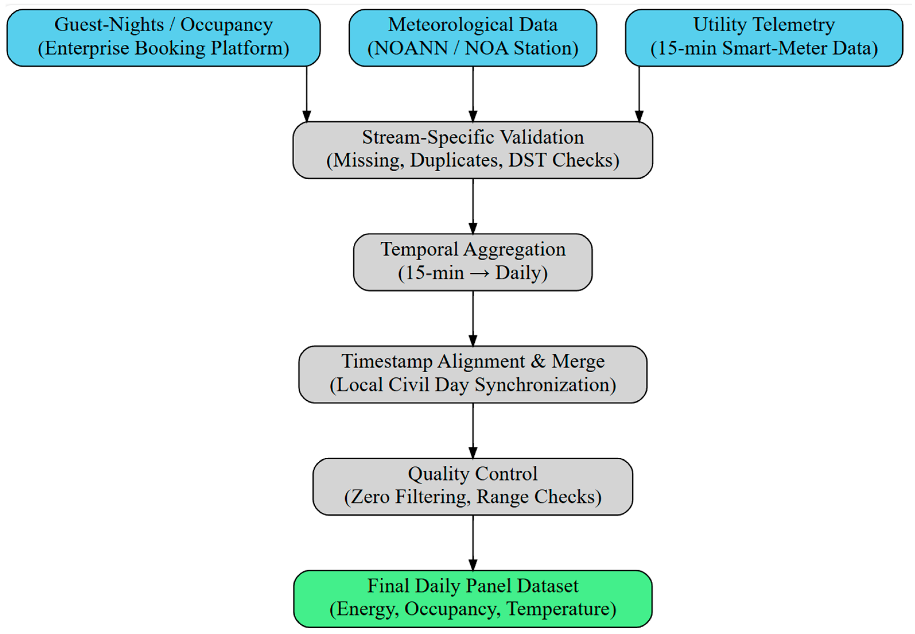
NOA meteorological station	Air temperature (°C)	Hourly	Daily mean	NOA network

summarizes the characteristics of each data stream, while Figure 1 illustrates the automated workflow for their acquisition, validation, and synchronization.

The local distribution system operator (HEDNO) exposes quarter-hour interval readings for the primary service meter through a secure API. Raw intervals are retrieved in local time and aggregated into calendar-day import active energy by summing intraday increments. Daylight–saving transitions are validated by checking the expected number of intervals per civil day (96 on standard days; 92 or 100 on transition days).

Daily guest-night totals are obtained from the property’s enterprise booking platform through an authenticated endpoint. Bulk edits and cancellation updates are automatically filtered to maintain consistency with the final occupancy records used in sustainability reporting.

Ambient temperature is sourced from the NOA automatic weather-station network, which provides dense spatial coverage across Greece and has been systematically validated for research applications [30]. The nearest station with stable data availability is selected; sub-daily readings are normalized to local time and aggregated into mean daily temperature values. The update cadence and reliability of the NOA network make it suitable for building-scale forecasting tasks that depend on timely local meteorological drivers.

Following stream-specific validation, the three datasets are synchronized on a common local-day timestamp to form a single harmonized panel. Quality-control checks include duplicate-timestamp detection, monotonicity validation for cumulative counters, and zero-value filtering near daylight–saving boundaries. Figure 1 summarizes this workflow, emphasizing the standardized validation and merging sequence applied to all incoming data.

A small excerpt of the final dataset is presented in

Table 2. Excerpt of the final dataset.

Date	Daily Active Energy (kWh) (Indexed)	Guest-Nights (Indexed)	Mean Temp (°C)
1 April 2022	103.6	39	18.9
2 April 2022	112.5	62	16.9
3 April 2022	125.5	82	14.9
4 April 2022	132.8	92	10.8
5 April 2022	131.1	100	10.9

, illustrating the anonymized daily structure used for model training. Numerical values are indexed to preserve confidentiality while maintaining proportionality.

While the analysis focuses on a single hotel, the selected property is representative of a mid-size Mediterranean asset in terms of electrical infrastructure, occupancy patterns, and climatic exposure. Its load composition reflects the operational mix typical of resort-scale facilities—HVAC, food and beverage and guest services—driven by occupancy intensity and exogenous factors like outdoor temperature. The pipeline’s modular architecture allows retraining on other properties with minimal configuration changes, ensuring its adaptability across assets that share similar data structures and operational drivers. This design acknowledges that consumption–temperature relationships may vary among hotels due to scale or microclimate differences, yet emphasizes reproducibility and transferability over one-off optimization. By focusing on transparent data handling and open experiment tracking, the framework establishes a replicable methodological foundation for broader hotel-sector forecasting and portfolio-scale generalization.

3.2. Data Ingestion and Alignment

The pipeline ingests three heterogeneous sources:

• Utility interval telemetry, representing daily active energy imports at the main grid connection point.
• Guest-night counts as an occupancy proxy.
• Meteorological station records, providing the mean daily air temperature.

To establish comparability, all streams were synchronized to the local civil day using timezone-aware timestamps. Raw timestamps were parsed into canonical formats, and numeric fields were coerced into floating-point types. Locale-specific decimal commas were standardized into dotted floats. A row-screening stage eliminated records with missing values in critical fields (energy, temperature, timestamp) or with implausible zeros, which would otherwise bias scaling or model fitting.

Finally, to address confidentiality restrictions associated with enterprise operations, absolute values of Daily Active Energy (kWh) and Guest-nights were masked using a mean-based index transformation (value ÷ mean × 100). This intervention preserves relative variability, correlation structure, and seasonality, while preventing disclosure of proprietary magnitudes. As the transformation is linear, inferential validity (e.g., correlation coefficients, regression slopes, and forecasting performance) is unaffected, and the resulting dimensionless series remain fully suitable for exploratory and predictive analysis. Techniques similar to such anonymization have been shown to preserve forecasting performance in recent studies of anonymized load profiles [29].

3.3. Exploratory Data Analysis

This section summarizes the empirical patterns revealed by the analysis. After basic quality control (numeric coercion, timestamp parsing, and removal of zero or missing values), three daily variables are retained: Daily Active Energy (kWh), Guest-nights, and Temperature (°C) from the nearest meteorological station. Public holidays were not included as an additional feature because the resort’s all-inclusive operational pattern maintains stable activity levels across holidays; daily load is primarily driven by occupancy and temperature. All reported results are computed on this cleaned daily panel, following best practices in building-energy forecasting and correlation input-screening workflows [17].

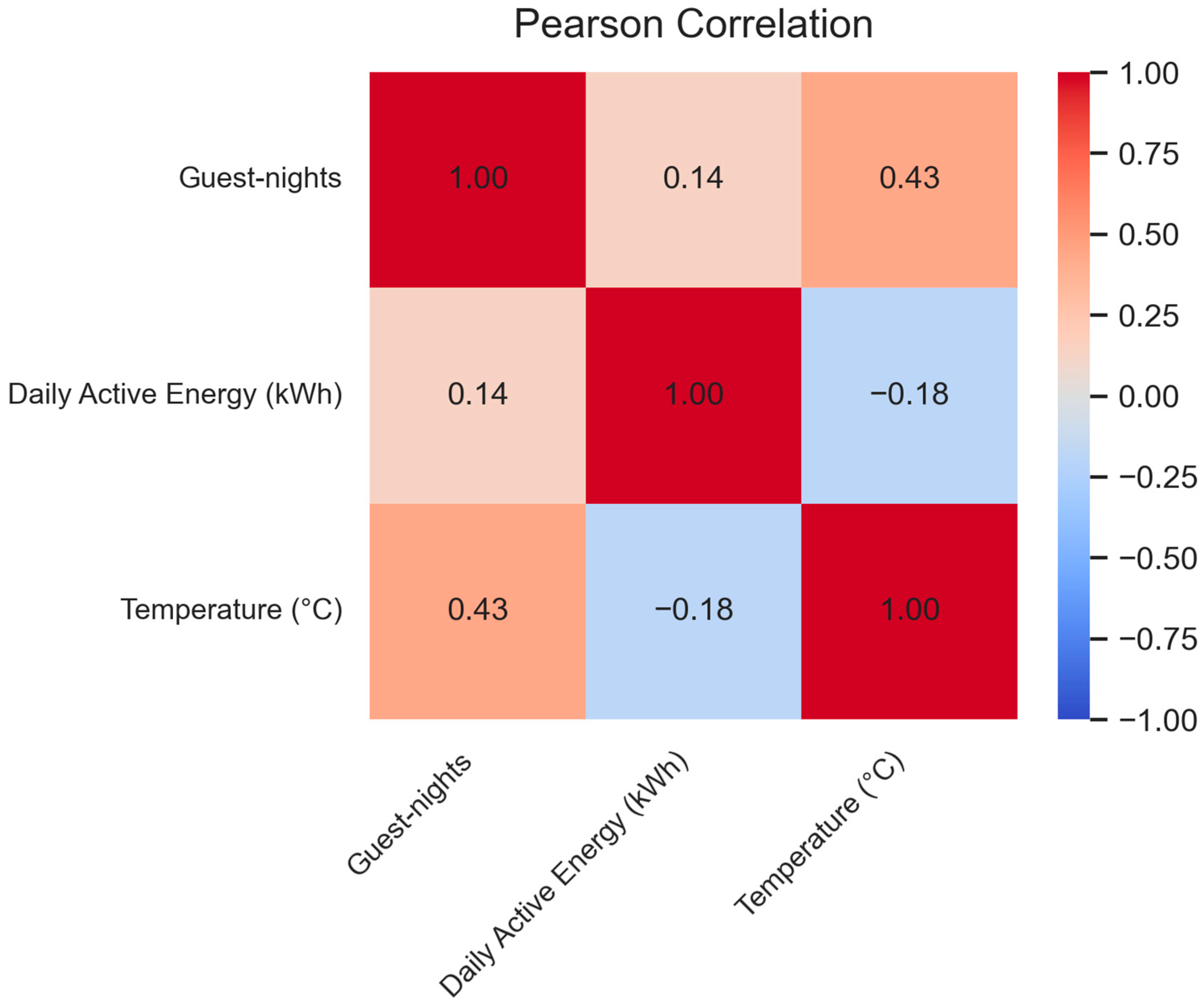
Figure 2 presents the Pearson correlation matrix, which captures the linear relationships among the three variables. Spearman and Kendall correlations were also examined but showed consistent directional patterns and relative magnitudes; therefore, to avoid redundancy and improve readability, only the Pearson matrix is displayed here.

The correlation between energy and guest-nights is positive but modest (Pearson = 0.14), indicating that occupancy contributes to daily variability yet is not the sole driver—consistent with findings in real-time energy consumption studies that incorporate occupancy and weather [18]. Temperature exhibits a moderate positive association with guest-nights (Pearson = 0.43), reflecting seasonality in guest activity. In contrast, the aggregate energy–temperature correlation is weakly negative (Pearson = −0.18), suggesting a non-monotonic relationship between load and temperature. This pattern is expected when both heating and cooling regimes are pooled, since opposing seasonal effects tend to cancel in linear correlation analysis.

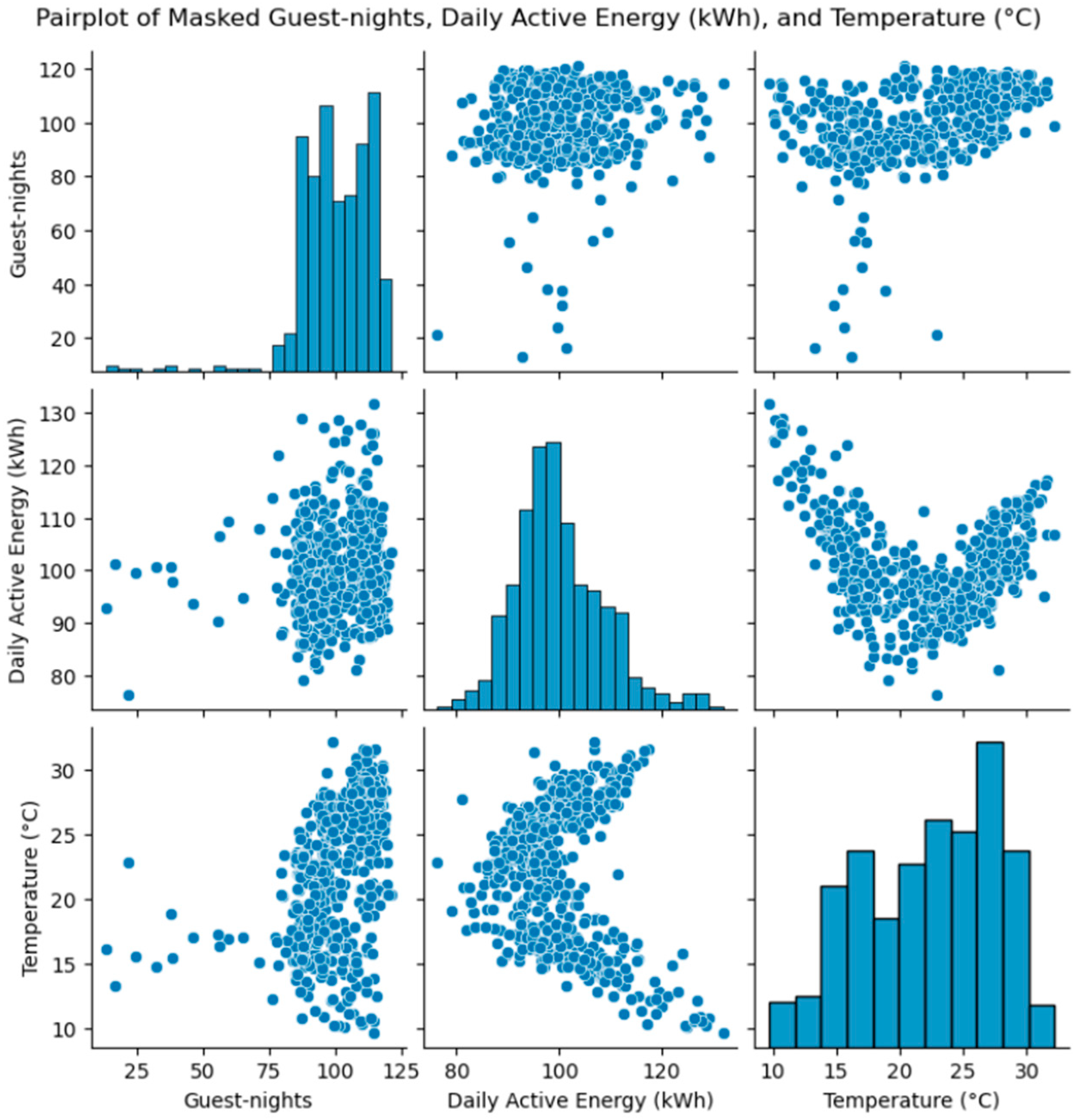
The scatter-matrix Figure 3 qualitatively supports these findings. Energy versus temperature exhibits a V-shaped pattern: consumption is elevated at lower and higher temperatures relative to the shoulder season, reflecting the superposition of heating and cooling demands at different times of the year [19]. Energy versus bookings shows a generally increasing cloud with heteroskedasticity (larger spread at higher occupancy), implying interactions with exogenous drivers such as weather and calendar effects. The marginal histograms indicate concentrated occupancy regimes with occasional low-activity days, an energy distribution with a pronounced main mode and a high-load tail, and temperatures spanning roughly the 10–30 °C range without extreme outliers.

To further assess whether temperature–energy dependence strengthens under higher thermal loads, correlations were recalculated after progressively excluding cooler days. The maximum correlation occurs near 22.2 °C, where the energy–temperature relationship peaks at approximately 0.72 (Pearson). This confirms that the weak global correlation arises from the coexistence of distinct operational regimes rather than a lack of dependence.

Although the scatter-matrix in Figure 3 displays a V-shaped relationship, this should not be interpreted as symmetric heating and cooling dominance. The distribution of daily temperatures within the April–October interval is highly asymmetric, with only a small number of low-temperature days remaining at the margins of the warm season. During these few cooler days, the property’s heated swimming pools and partial space-heating systems are active, temporarily increasing the electrical load. This explains the apparent rise in consumption at lower temperatures even within an otherwise cooling-dominated period.

Overall, once these infrequent heating-pool days are down-weighted or excluded, the relationship becomes strongly positive, reflecting the expected cooling-driven regime typical of Mediterranean hotels. Such regime-aware diagnostics are essential before feature design and model selection in short-term load forecasting [19].

The combination of weak global linear correlation yet clear curvature in energy–temperature space, modest but consistent dependence on guest-nights, and seasonal organization in the scatter plots supports a feature set that includes short lags of the target, calendar indicators, and exogenous drivers (temperature and guest-nights), together with a sequence model capable of learning nonlinear and interaction effects—choices consistent with established literature and recent applied case studies [19].

3.4. Feature Construction

The core predictive task—forecasting daily active energy demand—requires careful feature design. First, autoregressive lags of the target variable were constructed. These lag features capture short-term persistence and thermal inertia effects, which are especially pronounced in energy use for hospitality facilities [27].

Second, calendar encodings were derived from the civil timestamp. Month and day-of-week attributes were extracted and transformed into one-hot encoded indicator variables (with one reference category dropped to avoid multicollinearity). These encodings help capture systematic patterns such as seasonality and weekend effects, which are well-documented in short-term load forecasting [26].

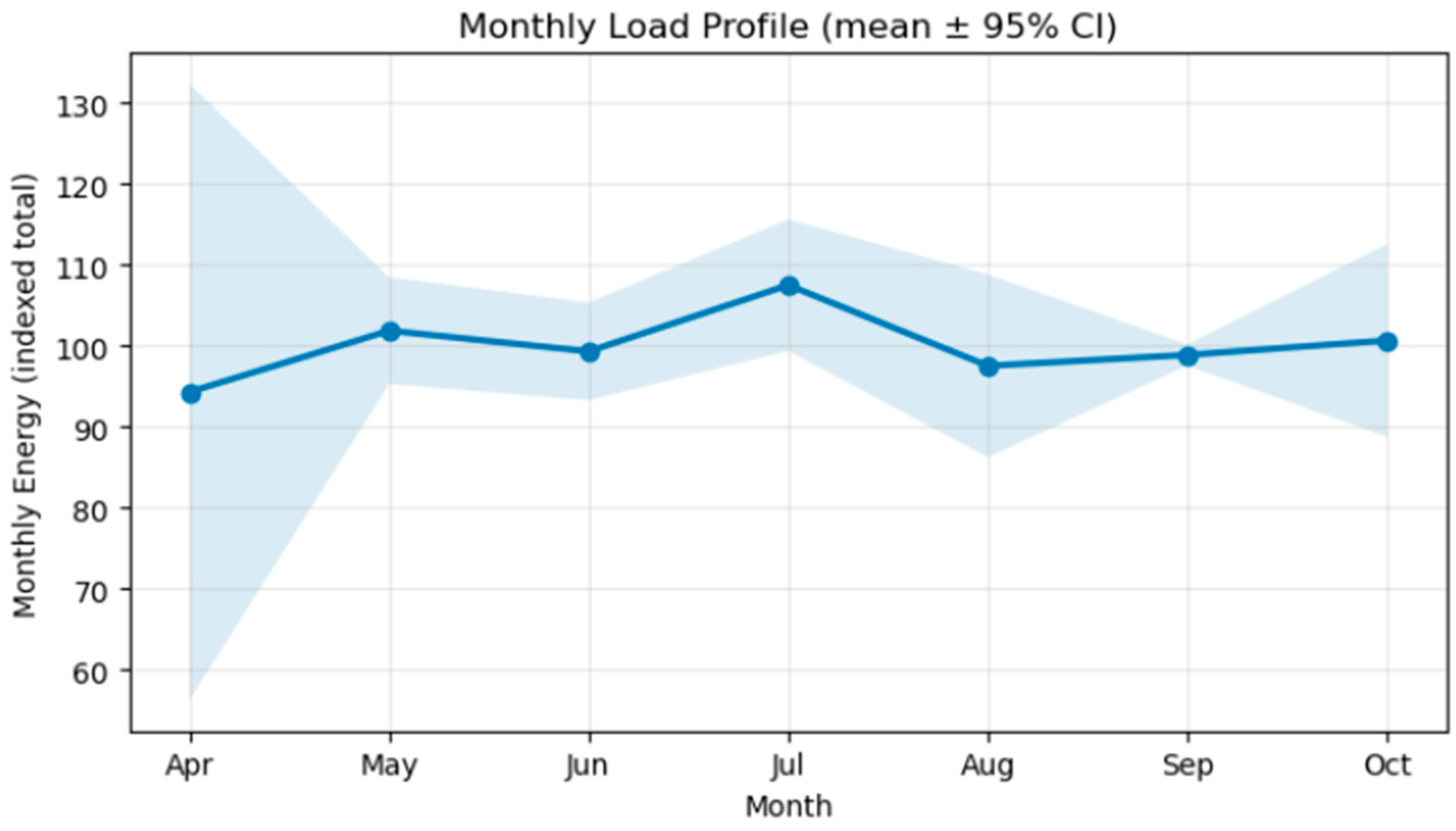
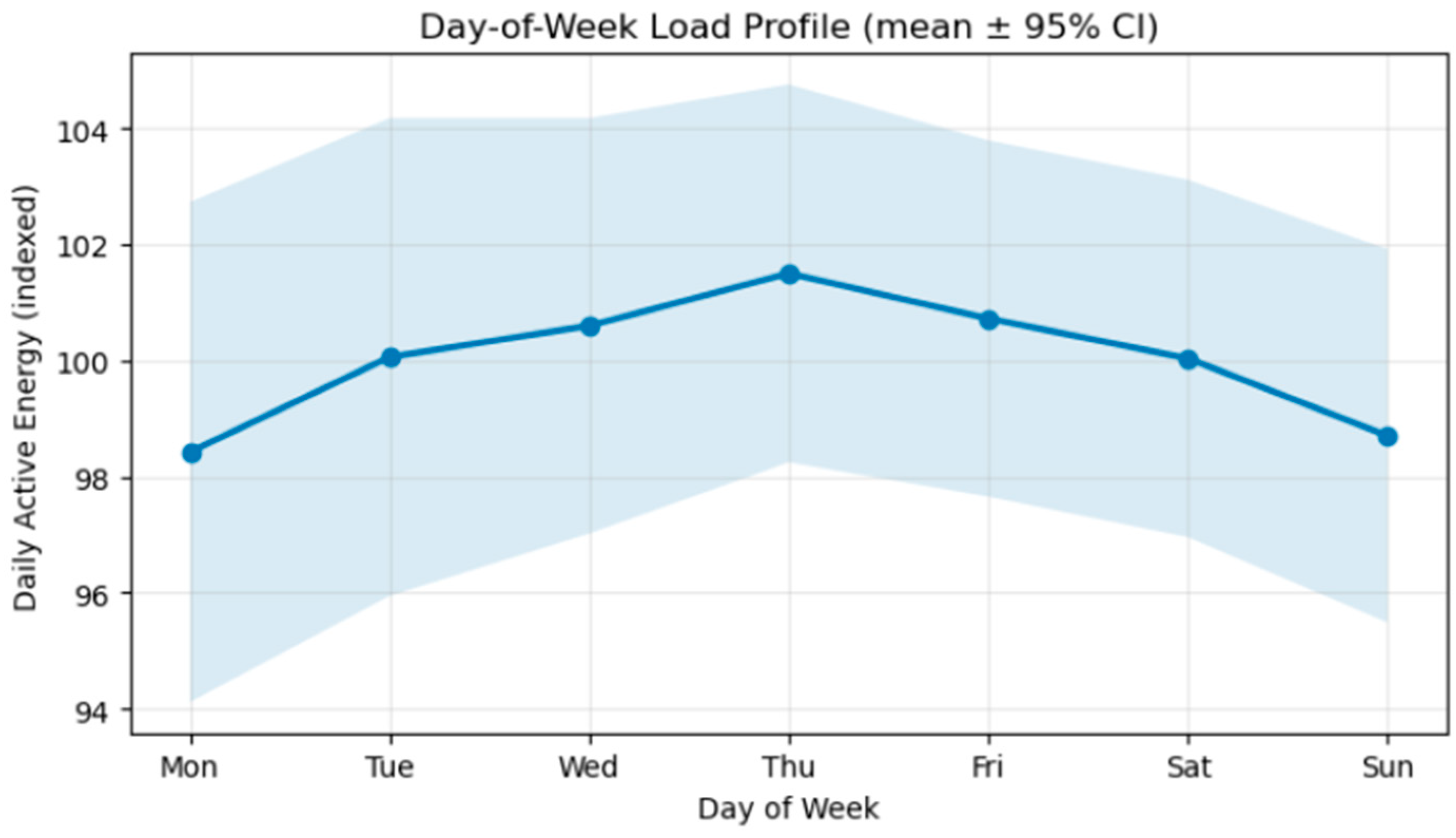
To further illustrate calendar-related variability, Figure 4 and Figure 5 present the empirical profiles of monthly and day-of-week electricity demand, aggregated from the harmonized daily dataset. Both plots display mean values with 95% confidence intervals, derived from data within the April–October interval.

The monthly load profile (Figure 4) shows a clear seasonal pattern, with energy consumption rising steadily from spring toward its peak in July and August—months characterized by elevated cooling loads—and decreasing again toward October. This pattern is consistent with the climate-driven seasonality expected for Mediterranean resort operations.

The day-of-week load profile, Figure 5, exhibits systematic intra-week variation, with slightly higher average demand from mid-week to Friday, followed by a decline on weekends. This behavior reflects operational scheduling, guest turnover cycles, and ancillary service activity typical of hospitality facilities.

Together, these results confirm that both month and day-of-week effects contribute meaningfully to the variability of daily load. Accordingly, both are encoded as one-hot calendar features in the forecasting model to capture recurring seasonal and operational patterns.

Third, exogenous drivers were introduced. These include daily mean temperature, which reflects climatic load, and guest-night counts, which approximate occupancy intensity. Finally, rows rendered incomplete by lagging were removed to ensure fully observed samples. The deliverable of this step is a structured engineered feature matrix at daily resolution, where all predictors are aligned with the target.

3.5. Normalization and Schema Control

To stabilize optimization and prevent data leakage, a two-scaler strategy was implemented. All predictor variables, including lags, temperature, guest-nights, and calendar encodings, were scaled into the range (0, 1) using a general Min–Max scaler. The target variable was scaled separately, with the scaler fit only on the training subset. This approach prevents information leakage from future (test) data into model fitting, a standard safeguard in energy data pipelines [7]. To enforce schema consistency across training, validation, and inference phases, the pipeline persists:

• An ordered post-encoding feature list, ensuring that one-hot expansions and feature ordering remain identical across runs
• Both fitted scalers (input and target). This design enables fully reproducible transformations when models are deployed, which has been highlighted as a requirement for transparent energy AI systems [16].

The outputs of this stage include the general input scaler, the target scaler, and the ordered feature schema artifact, all serialized as artifacts for experiment tracking and later inference.

4. Methodology

4.1. Theoretical Framework and Model Formulation

The proposed forecasting model adopts a supervised deep learning framework designed to predict next-day electricity demand using historical consumption, occupancy, and meteorological data. The workflow integrates three validated and synchronized data streams:

(i)

distribution-operator smart-meter telemetry,

(ii)

enterprise booking records (as an occupancy proxy), and

(iii)

daily mean temperature derived from the NOA network.

All preprocessing, feature construction, and model training steps were implemented in Python 3.11.9 using open-source libraries, ensuring reproducibility and transparency.

The modeling architecture combines sequential and contextual information to capture nonlinear dependencies between electricity use, occupancy intensity, and weather fluctuations. Input features include short target lags, calendar encodings, and exogenous variables (temperature and guest-nights), which are concatenated into a unified tensor and supplied to a two-layer recurrent neural network composed of stacked LSTM units.

The LSTM extends the standard RNN through three gating mechanisms that regulate the flow of information across time. At each time step t, given an input vector x_t and previous hidden state h_t−1, the unit performs the following computations.

$$f_t=\sigma \left(W_f{x}_t+U_f{h}_{t-1}+b_f\right)$$

(1)

$$i_t=\sigma \left(W_i{x}_t+U_i{h}_{t-1}+b_i\right)$$

(2)

$${\mathrm{ĉ}}_t=tanh\left(W_c{x}_t+U_c{h}_{t-1}+b_c\right)$$

(3)

$$c_t=f_t\odot c_{t-1}+i_t\odot {\mathrm{ĉ}}_t$$

(4)

$$o_t=\sigma \left(W_o{x}_t+U_o{h}_{t-1}+b_o\right)$$

(5)

$$h_t=o_t\odot tanh\left(c_t\right)$$

(6)

As shown in Equation (1), the forget gate f_t determines how much of the previous cell state c_t−1 should be retained, thereby controlling the rate at which historical information decays and allowing the network to discard irrelevant patterns while preserving meaningful long-term dependencies. In Equation (2), the input gate i_t regulates the inflow of new information into the memory cell, determining which components of the current input are stored so that relevant short-term variations—such as changes in occupancy or ambient temperature—are effectively captured. Equation (3) defines the candidate cell state ĉ_t, which generates potential new memory content derived from the current input and the previous hidden state, representing contextual information that can complement or partially overwrite existing memory. As formulated in Equation (4), the cell state update c_t integrates the retained portion of the old memory and the newly scaled candidate information, forming the updated internal state that combines historical context with recently observed dynamics. According to Equation (5), the output gate o_t controls which parts of this updated memory are revealed to the hidden state, filtering internal information to determine how much of the cell state contributes to the model’s output. Finally, Equation (6) defines the hidden state h_t, which represents the output of the LSTM unit at each time step, encapsulating both short- and long-term dependencies and passing this temporal context to subsequent layers. Collectively, these mechanisms enable the LSTM network to balance memory retention, information filtering, and nonlinear transformation—properties essential for modeling daily electricity demand patterns shaped by interacting climatic and behavioral drivers Algorithm 1.

Algorithm 1. LSTM-Based Day-Ahead Electricity Forecasting Framework

Input: Historical time series of electricity consumption Et, occupancy proxy Ot, and ambient temperature Tt. Output: Predicted next-day electricity demand Ēt+1. Aggregate and synchronize raw data streams (Et, Ot, Tt) to daily resolution. Perform data cleaning and handle missing values and daylight–saving irregularities. Construct lagged features Et−1, Et−2, …, Et−L and encode exogenous variables (calendar dummies, Ot, Tt). Normalize all input features using Min–Max scaling:             x′ = (x − xmin)/(xmax − xmin). Split the dataset chronologically into training and testing subsets to avoid data leakage. Initialize a two-layer LSTM network LSTM(U1, U2, p_d) with dropout rate p_d and a dense regression head f_θ. Train the model by minimizing the mean squared error (MSE):             𝓛(θ) = (1/N) Σt=1N (Et − Ēt)2             using the Adam optimizer with early stopping based on validation loss. Evaluate predictive accuracy on the test set using the following metrics:             RMSE = √[(1/N) Σt=1N (Et − Ēt)2]             MAE = (1/N) Σt=1N |Et − Ēt|             MAPE = (100/N) Σt=1N (|Et − Ēt|/Et). Log all hyperparameters, metrics, and artifacts (θ, 𝓛, RMSE, MAE, MAPE) to ensure experiment reproducibility and auditing.

In summary, this theoretical framework integrates autoregressive memory through stacked LSTM layers with contextual drivers such as temperature, occupancy, and calendar effects. By combining transparent preprocessing, leakage-safe validation, and MLflow-based tracking, the approach ensures both scientific reproducibility and operational relevance. The next subsections detail the data ingestion, feature construction, and temporal-split procedures that operationalize this formulation within the implemented forecasting pipeline.

4.2. Supervised Sequence Framing and Temporal Split

The forecasting problem is setup as a supervised sequence learning task. Each training sample uses a sliding window of L preceding daily observations to predict energy demand on day t + 1. This converts the daily feature table into 3-D arrays with shape:

• X: [num_samples, L, num_features]
• y: [num_samples, 1]

Define z(t) as the feature vector for day t (length = num_features) and y(t) as the scaled target (energy) for day t. For each index t, a single sample is:

• Input sequence: X_sample = [z(t − L + 1), z(t − L + 2), …, z(t)] (an L-by-num_features matrix)
• Target: y_sample = y(t + 1) (a scalar)

To avoid leakage, we apply a strictly chronological split. The dataset was divided chronologically into 80% training and 20% testing subsets based on the aligned target dates to avoid temporal leakage. The training period spans 8 April 2022–1 May 2024 (452 days), while the hold-out test period covers 2 May–23 August 2024 (114 days). There is no shuffling, so temporal order is preserved [1].

4.3. Model Specification

The forecasting framework is based on a stacked recurrent neural network (RNN) using the LSTM architecture. LSTMs were chosen due to their ability to capture nonlinear temporal dependencies in sequential data, such as persistence, occupancy-driven effects, and weather-related variability in energy demand [23,27].

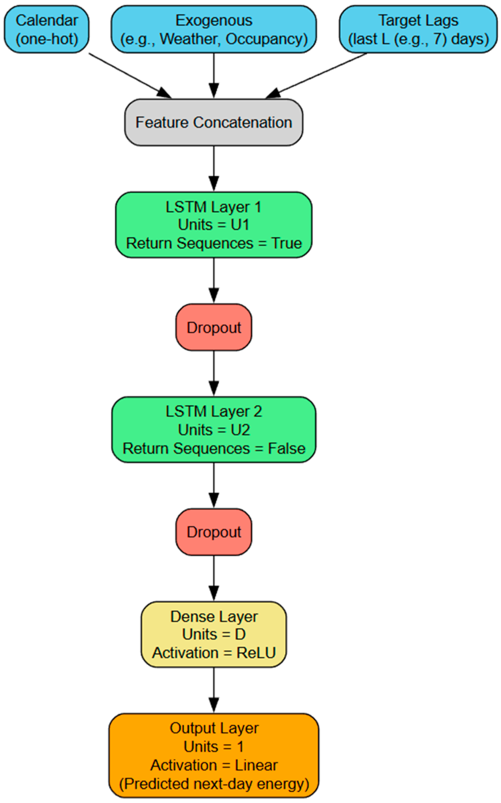
The network Figure 6 consists of two recurrent layers. Each layer is parameterized with 40–80 hidden units, depending on the sampled configuration. To mitigate overfitting, dropout layers are interleaved with dropout rates between 0.1 and 0.3. The recurrent stack is followed by a compact dense regression head, comprising one hidden layer with 16–48 ReLU-activated units, and a single output neuron that predicts the next day’s energy demand.

The model is compiled with the Adam optimizer, tested at learning rates of 0.001, 0.0005, and 0.0001. The training objective is the MSE, suitable for penalizing large deviations in forecasts. To prevent overfitting and accelerate convergence, early stopping is employed. Training is halted when validation loss fails to improve for 10–30 epochs, and the weights corresponding to the lowest validation error are restored. Reproducibility measures include fixed random seeds across all packages (NumPy, TensorFlow, Python random) and polite GPU memory allocation, which prevents monopolization of GPU resources while ensuring stable execution.

4.4. Hyperparameter Search

To select an effective architecture, we employed a bounded random search that samples from the predefined space of models and training settings. Compared with exhaustive grid search—which scales poorly with dimensionality—random sampling offers broad, unbiased coverage of the space at a fixed computational budget while remaining tractable [16]. The search space comprised eight hyperparameters

Table 3. Hyperparameter search space explored for the LSTM forecasting model.

Hyperparameter	Search Space	Notes
Look-back window (L)	{7, 10, 14}	Number of prior days used as input
LSTM units (layer 1)	{40, 55, 64, 80}	Width of first recurrent layer
LSTM units (layer 2)	{40, 55, 64, 80}	Width of second recurrent layer
Dropout rate	{0.1, 0.2, 0.3}	Regularization against overfitting
Dense head width	{16, 25, 32, 48}	Hidden units in regression head
Batch size	{16, 32, 64}	Mini-batch size for optimization
Epochs	{20, 40, 80}	Early stopping caps effective epochs
Patience	{10, 20, 30}	Epochs tolerated without improvement
LR	{0.001, 0.0005, 0.0001}	Adam optimizer initial learning rate

, and each trial followed the same preprocessing, scaling, and temporal split. We evaluated up to 40 distinct configurations, ensuring comparability across runs.

To move from exploration to performance ranking, every configuration was assessed on the hold-out test span using a consistent, leakage-safe protocol. We prioritized RMSE (7) as the primary selection criterion, reflecting sensitivity to large deviations that matter operationally in kWh, calculated as follows:

$$\mathrm{R}\mathrm{M}\mathrm{S}\mathrm{E}=\sqrt{{\displaystyle \frac{1}{\mathrm{n}}}\sum _{\mathrm{i}=1}^{\mathrm{n}}{\left({\mathrm{y}}_{\mathrm{i}}-\widehat{{\mathrm{y}}_{\mathrm{i}}}\right)}^2}$$

(7)

Two secondary metrics, MAE (8) and MAPE (9), were used to corroborate the ranking and check robustness across absolute and relative error scales, calculated as follows:

$$\mathrm{M}\mathrm{A}\mathrm{E}={\displaystyle \frac{1}{\mathrm{n}}}\sum _{\mathrm{i}=1}^{\mathrm{n}}\left|{\mathrm{y}}_{\mathrm{i}}-\widehat{{\mathrm{y}}_{\mathrm{i}}}\right|$$

(8)

$$\mathrm{M}\mathrm{A}\mathrm{P}\mathrm{E}={\displaystyle \frac{100}{\mathrm{n}}}\sum _{\mathrm{i}=1}^{\mathrm{n}}\left|{\displaystyle \frac{{\mathrm{y}}_{\mathrm{i}}-\widehat{{\mathrm{y}}_{\mathrm{i}}}}{{\mathrm{y}}_{\mathrm{i}}}}\right|$$

(9)

All runs were tracked in MLflow, with parameters, metrics, and diagnostic plots archived; artifacts (trained model, input and target scalers, and the ordered feature schema) were persisted alongside a consolidated CSV of all trials. This process yields the best-performing model and, importantly, exposes how forecast accuracy varies with look-back length, recurrent layer width, and dropout regularization, informing both selection and future design choices [16,31].

5. Results

5.1. Hyperparameter Search and Top-10 Leaderboard

A bounded random search evaluated 40 unique configurations under an identical preprocessing pipeline, separate input/target scaling, and a leakage-safe chronological split. Runs were ranked by RMSE on the hold-out span, with MAE and MAPE used as secondary checks.

Table 4. Top-10 LSTM hyperparameter configurations ranked by RMSE on the hold-out test set.

Run_Name	Look Back	Lstm Units 1	Lstm Units 2	Dropout	Dense1	Batch Size	Epochs	Patience	LR	RMSE	MAE	MAPE (%)
LSTM_Hyperparam Trial_19	10	80	40	0.1	32	32	20	10	0.001	4.710	3.479	3.290
LSTM_Hyperparam Trial_11	7	64	80	0.2	16	16	80	30	0.0005	4.852	3.846	3.628
LSTM_Hyperparam Trial_39	10	64	55	0.2	32	64	80	30	0.001	4.993	3.916	3.697
LSTM_Hyperparam Trial_17	10	40	64	0.3	25	64	20	30	0.0005	5.158	4.217	4.014
LSTM_Hyperparam Trial_25	7	55	64	0.3	48	16	80	10	0.0001	5.265	4.205	3.973
LSTM_Hyperparam Trial_22	7	64	80	0.3	32	32	80	20	0.001	5.267	4.143	3.897
LSTM_Hyperparam Trial_21	14	80	55	0.2	48	16	80	30	0.0001	5.290	4.268	4.010
LSTM_Hyperparam Trial_26	14	80	55	0.2	48	16	20	10	0.0001	5.289	4.267	4.010
LSTM_Hyperparam Trial_34	7	40	40	0.1	16	64	20	30	0.001	5.305	4.307	4.067
LSTM_Hyperparam Trial_32	10	80	64	0.2	48	16	20	20	0.001	5.508	4.456	4.175

lists the Top-10 configurations together with their MLflow run names to ensure auditability.

Best run—Trial_19 is the top performer with RMSE 4.71, MAE 3.48, and MAPE 3.29%. It uses look_back = 10, asymmetric recurrent widths (80 → 40), dropout = 0.1, dense1 = 32, batch_size = 32, epochs = 20 with patience = 10, and LR = 1 × 10⁻³. Tight clustering is evident because ranks 1–3 are within approximately 0.28 RMSE of one another, indicating multiple near-optimal settings. The effect of look-back is consistent: strong performers occur at L = 10 (ranks 1, 3, 4, 10) and L = 7 (ranks 2, 5, 6, 9), with L = 14 appearing at ranks 7–8; extending beyond 10 days did not systematically improve accuracy in this dataset. With respect to dropout, the best model uses 0.1; 0.2 appears consistently competitive (ranks 2–3, 7–8, 10); 0.3 tends to underperform slightly (ranks 4–6). Regarding layer widths, several top entries favor a wider first LSTM (80) followed by a narrower second LSTM (40–64), suggesting benefit from a rich temporal encoding followed by a consolidating layer. For the learning rate, 1 × 10⁻³ is prevalent among the strongest runs (ranks 1, 3, 6, 10), while 5 × 10⁻⁴ or 1 × 10⁻⁴ can also succeed depending on other settings. Trials 21 and 26 yield identical metrics with the same architecture and optimizer settings but different epoch/patience combinations, consistent with early-stopping dynamics.

5.2. Cross-Model Diagnostics

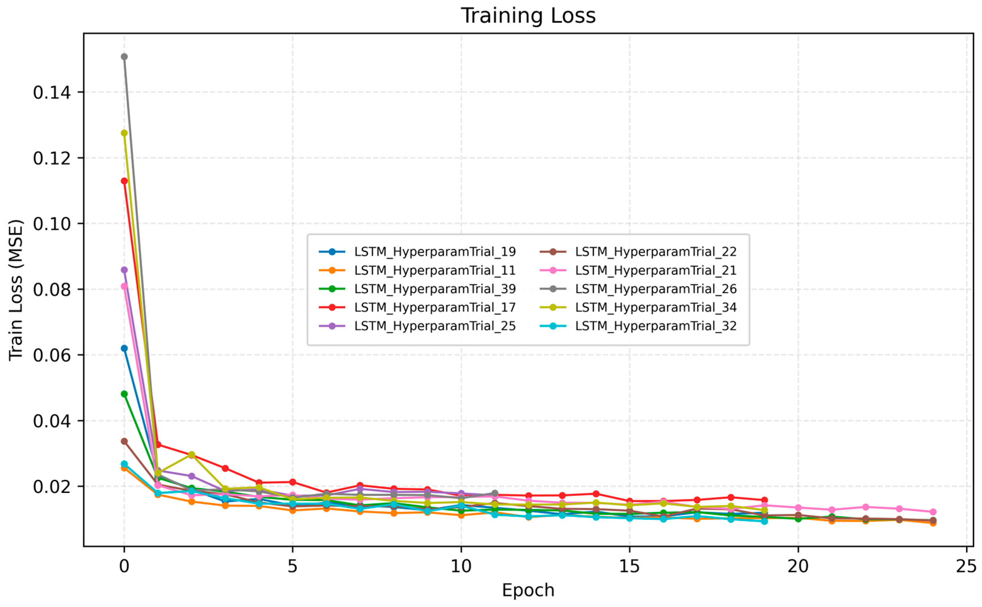
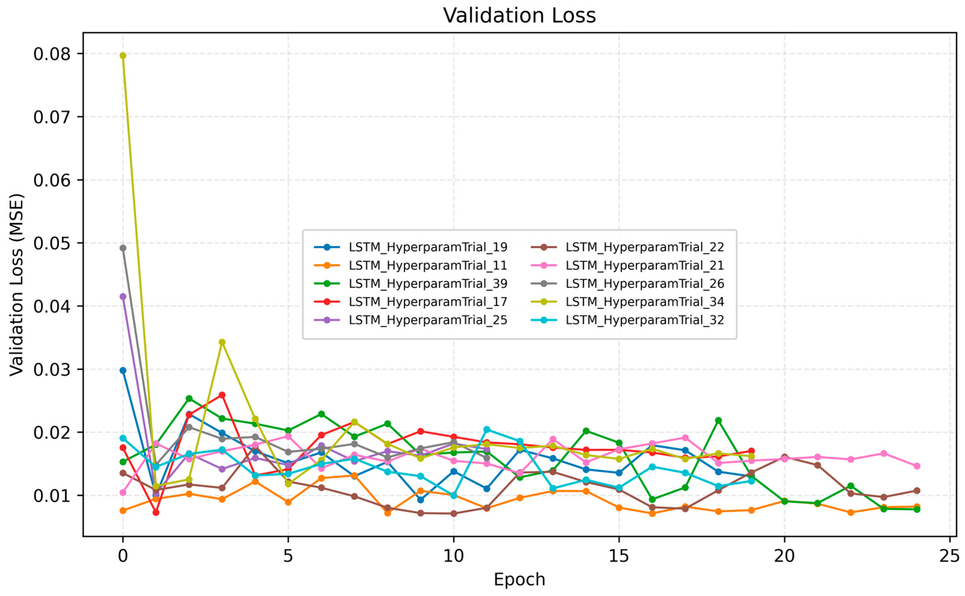
The MLflow dashboards for the Top-10 reveal consistent behavior. The training loss Figure 7 and validation loss Figure 8 show rapid decay in the first few epochs followed by a stable plateau; validation curves track training closely, indicating limited overfitting and effective early stopping across runs. Ranking stability is also apparent, because models that excel in RMSE typically also hold strong in MAE and MAPE, implying that improvements are not driven by outlier handling alone but by genuine overall fidelity.

5.3. Best Model

The top-performing configuration consists of two recurrent layers with asymmetric widths; a detailed layer-by-layer specification is provided in

Table 5. Layer-by-layer specification of the top-performing LSTM model.

Layer (Type)	Output Shape	Parameters	Notes
LSTM (lstm_156)	(None, 10, 80)	33,280	return_sequences = True
LSTM (lstm_157)	(None, 40)	19,360	return_sequences = False
Dropout (dropout_157)	(None, 40)	0	rate = 0.1
Dense (dense_156)	(None, 32)	1312	activation = ReLU
Dense (dense_157)	(None, 1)	33	activation = Linear
Total	—	53,985	All trainable

. The first LSTM layer contains 80 hidden units and returns full sequences over a 10-day look-back window, enabling the extraction of rich temporal dynamics. This is followed by a dropout layer (rate = 0.1) that reduces co-adaptation and mitigates overfitting. In the best-performing configuration, the look-back window was set to L = 10, meaning that each prediction used the previous ten days of input history. The per–time-step feature vector comprised 10 autoregressive lags, 6 day-of-week dummies, 6 month dummies, and 2 exogenous variables (temperature and guest-nights), yielding a total of 24 independent variables. After normalization, these were reshaped into a three-dimensional input tensor of shape (N, 10, 24) representing samples, time steps, and features, respectively. This explicit specification ensures full reproducibility of the model’s input dimensionality and aligns with standard practice in short-term load-forecasting architectures. The second LSTM layer compresses the representation to 40 units, effectively distilling salient features into a lower-dimensional latent space. A second dropout layer with the same rate further stabilizes training. The recurrent backbone is followed by a fully connected dense layer of 32 neurons with ReLU activation, which provides nonlinear transformation before the final output layer (linear activation, 1 unit) produces the one-step-ahead energy demand forecast. In total, the model contains 53,985 trainable parameters, a scale that balances learning capacity with computational efficiency.

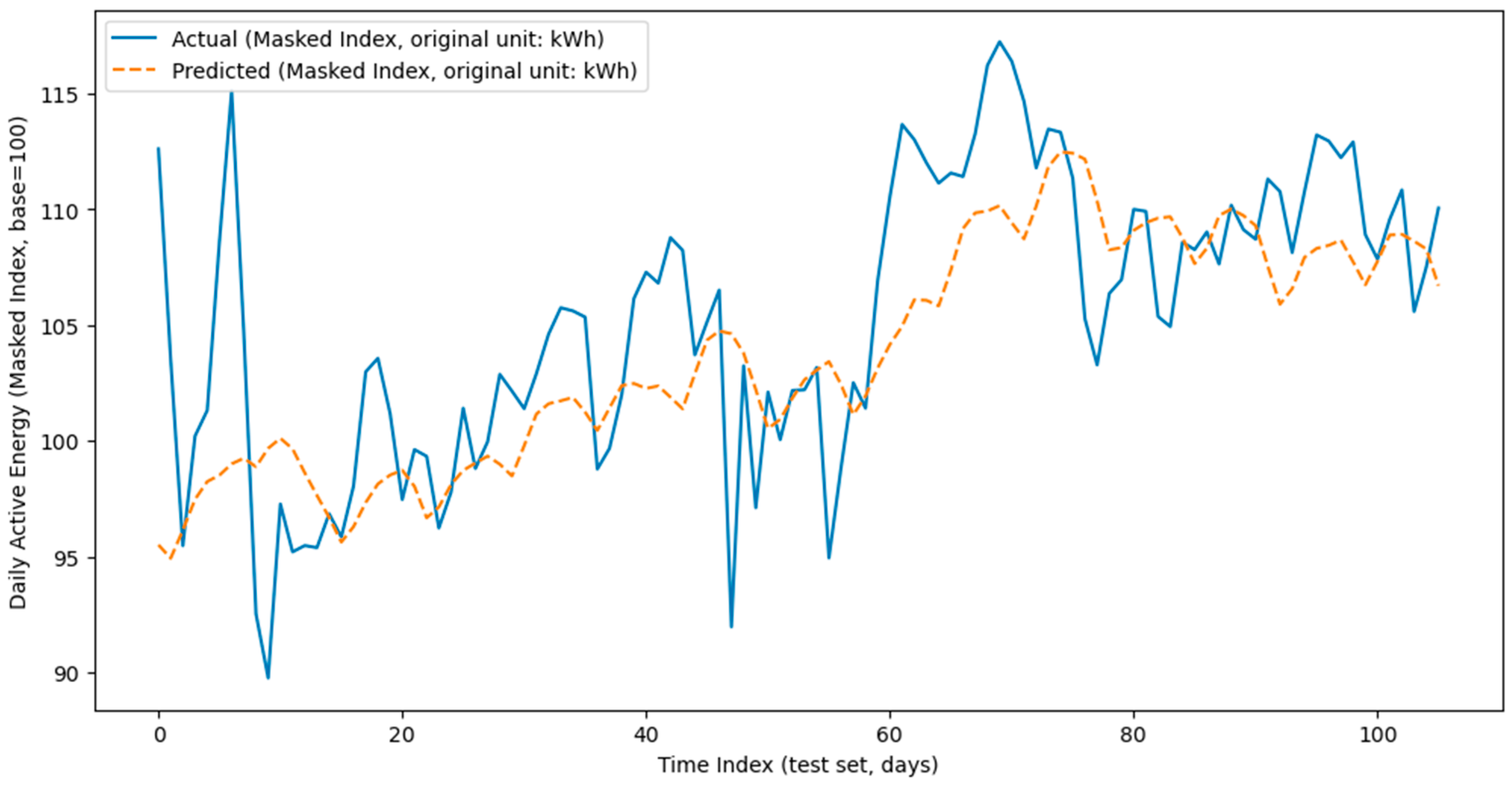
Training diagnostics support the appropriateness of this design. The actual versus predicted curves Figure 9 demonstrate that the model accurately follows the shape and magnitude of daily energy consumption, with only minor transient deviations.

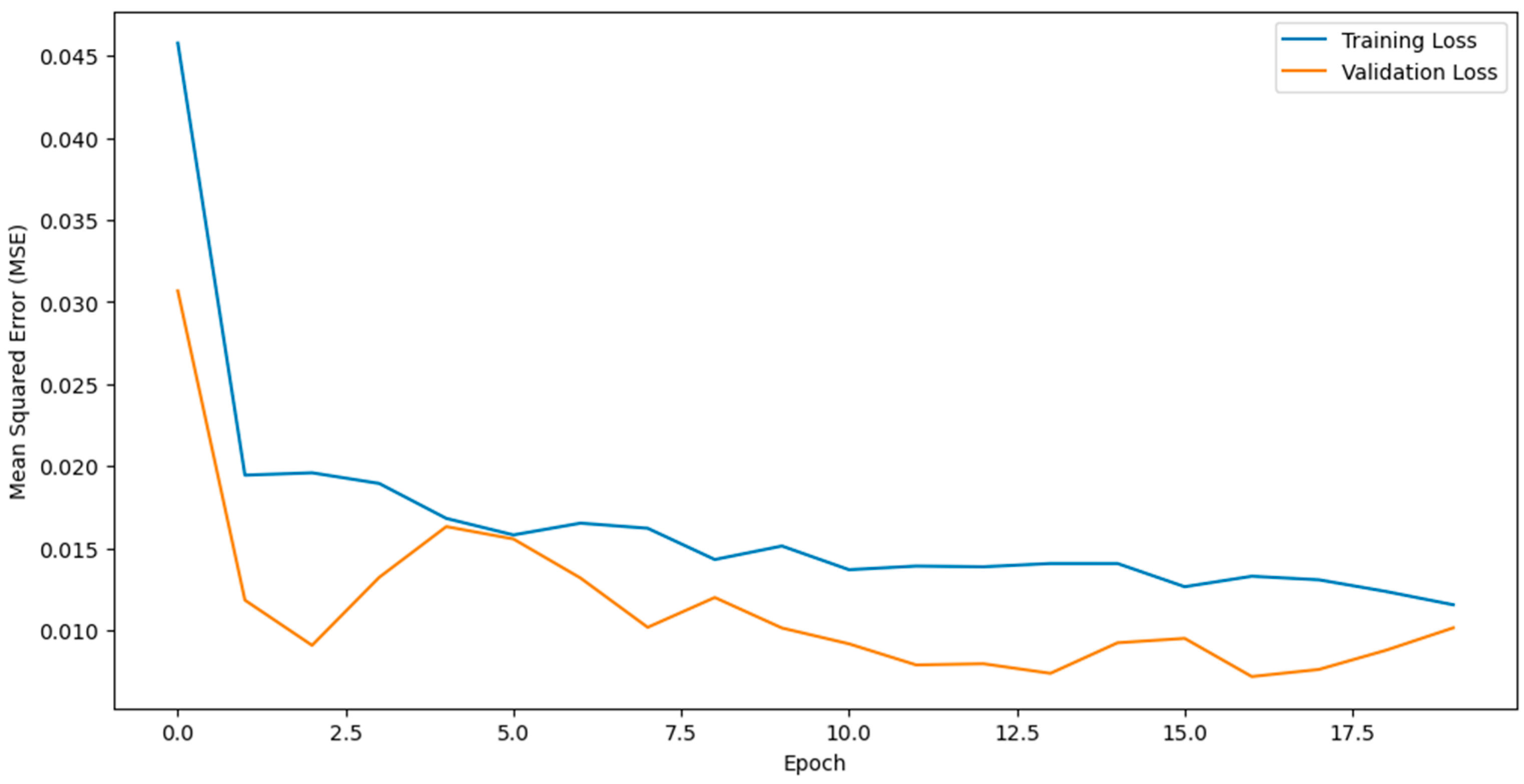
Training loss and validation loss curves, Figure 10, converge smoothly and remain tightly coupled, confirming the effectiveness of the dropout–early stopping combination in avoiding overfitting.

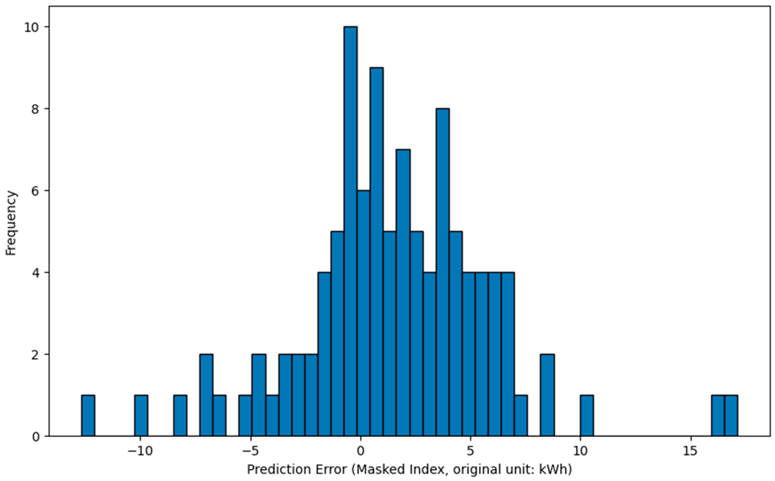
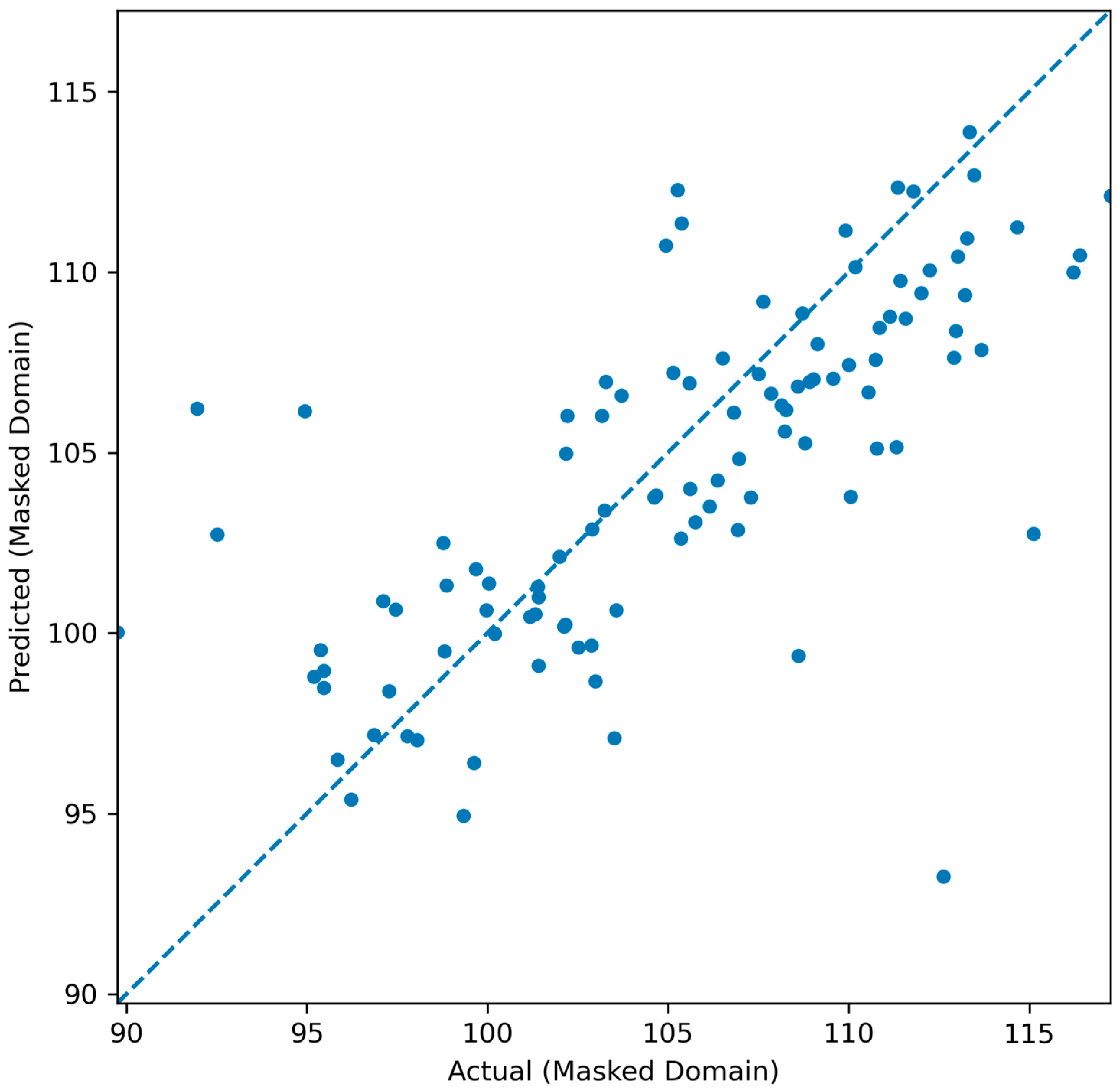
The error histogram reveals residuals centered around zero and symmetrically distributed Figure 11, while the parity plot Figure 12 indicates close alignment along the 45° identity line, with no systematic bias across the demand spectrum.

Overall, the Trial_19 architecture demonstrates that a medium-depth LSTM with asymmetric recurrent widths, modest dropout, and a compact dense head achieves robust generalization for hotel load forecasting. Its reproducibility is guaranteed by the persisted artifacts—serialized model weights, both scalers, the ordered feature schema, and MLflow-tracked parameters and metrics.

5.4. Baseline Benchmarks and Comparative Performance

To contextualize the predictive accuracy of the proposed LSTM model, a series of open-source statistical and machine-learning baselines were implemented and evaluated under identical experimental conditions. All baseline models were trained on the same masked dataset, using an index, ensuring full comparability with the LSTM pipeline, as all models shared the same chronological train–test split, input feature composition, and preprocessing workflow.

The benchmark suite comprised four representative classes of models widely used in energy forecasting literature: (i) linear regression models (Ridge and Lasso) to capture first-order linear dependencies; (ii) an ARIMAX (SARIMAX + exogenous variables) configuration representing classical statistical time-series methods; (iii) gradient-boosted trees (XGBoost) as a strong nonlinear ensemble learner; (iv) a Random Forest regressor as a transparent, open-source, non-parametric ensemble baseline. The comparative results on the masked test set are summarized in

Table 6. Comparative performance of open-source baseline models.

Model	RMSE	MAE	MAPE (%)
Linear (Ridge/Lasso)	8.171	7.094	4.21
ARIMAX (SARIMAX + exog)	12.735	11.032	6.47
XGBoost	9.936	8.581	5.04
Random Forest	8.997	7.612	4.48
LSTM (Proposed)	4.710	3.479	3.29

.

Overall, the results demonstrate that traditional regression and ensemble-based methods are capable of explaining a substantial portion of the temporal and exogenous variability in daily load, particularly the Random Forest, which performed comparably to the linear Ridge/Lasso regressors. However, the proposed LSTM achieved markedly superior accuracy, with RMSE = 4.71, MAE = 3.48, and MAPE = 3.29%, representing an improvement of approximately 42–47% in RMSE and 22–27% in MAPE compared with the strongest classical baselines. The LSTM also outperformed XGBoost 3.0.0 and ARIMAX by more than 50% and 60% in RMSE, respectively, confirming the limitations of tree-based and autoregressive models in capturing long-term nonlinear dependencies. These consistent gains underscore the LSTM’s capability to model sequential dynamics and complex interactions among occupancy intensity, temperature, and calendar effects that remain only partially accessible to static or weakly autoregressive frameworks. Furthermore, the use of uniform masking, schema standardization, and MLflow-based tracking ensures full methodological transparency and reproducibility, establishing the LSTM as both a technically robust and operationally auditable solution for hotel-scale energy forecasting.

6. Discussion

This study demonstrates that a compact, regularized LSTM pipeline—driven by distribution-operator telemetry, an occupancy proxy, and proximal meteorology—can produce accurate and stable day-ahead forecasts for a hotel-scale electrical load. The empirical picture is consistent across the architecture and data choices reported: temporal contexts of roughly one to two weeks suffice to encode the dominant short-memory effects; asymmetric recurrent widths efficiently compress sequence information without sacrificing fidelity; and modest dropout curbs overfitting while keeping training dynamics smooth. These conclusions rest on a leakage-safe chronological split and an auditable hyperparameter search; as documented above, the top configurations occupy a narrow accuracy band on the hold-out span—an encouraging signal for retraining under evolving regimes. The leaderboard patterns and diagnostics further corroborate that wider first-layer encodings followed by narrower second-layer distillation tend to generalize well, while dropout in the 0.1–0.2 range balances bias–variance trade-offs among the strongest trials.

Beyond point accuracy, the pipeline’s design decisions matter for governance, comparability, and repeatability. Persisted scalers, an ordered post-encoding schema, and full MLflow run artifacts render experiments exactly recomputable and directly transferable to new temporal windows or sibling assets. This auditability is a prerequisite for operational adoption when forecasts inform staff scheduling, HVAC setpoint policies, and procurement planning. In the language of ISO 50001 [32], the model supports the energy review by quantifying SEUs and exposing their temporal drivers; in practice, this should be coupled with targeted submetering of major end-uses (e.g., chiller plant, domestic hot water, kitchen, laundry, lighting) to isolate load components, validate SEU attribution, and assign end-use-specific EnPIs with defensible baselines and measurement-and-verification trails. Submetered streams also enable finer-grained variance analysis and post-intervention tracking—so that observed savings can be reconciled to specific measures rather than inferred at the whole-building meter alone—while the unified pipeline ensures those additional signals can be incorporated without disrupting schema consistency. When aligned with ISO 14068 [33] carbon accounting, the same forecasts and submeter-informed allocations provide ex-ante activity-data projections for Scope 2 planning, enable more precise procurement of green electricity or guarantees of origin, and furnish counterfactual baselines against which measured abatement (e.g., load shifting or on-site generation) can be more credibly attributed and reported

6.1. Limitations

Interpretation of the results should be bounded by several considerations. The dataset emphasizes cooling-dominated months; consequently, the learned mappings primarily reflect air-conditioning and ventilation regimes, while heating-season behavior and shoulder-season idiosyncrasies remain undersampled. The modeling scope centers on LSTM-family architectures; although appropriate for the available features and horizon, alternative temporal encoders—notably attention-based and hybrid designs—could capture long-range or regime-switching dependencies differently, and probabilistic specifications might communicate uncertainty more faithfully when exogenous signals are noisy. The feature space, intentionally pragmatic for operations, omits submetered end-use telemetry that would sharpen causal attribution and enable end-use-aware targeting of measures.

6.2. Future Work

Architecturally, comparative experiments across encoder–decoder attention, temporal convolution, and hybrid CNN–LSTM stacks can test whether broader receptive fields or cross-feature attention reduce error on volatile days; probabilistic training objectives together with conformal or quantile-based post-processing could yield calibrated intervals that operators convert into risk-aware schedules and hedging strategies. Methodologically, explainability [34,35,36] and verification should be promoted to first-class deliverables: routine publication of attribution dashboards, seasonal stability audits, and red-team stress tests would align the pipeline with best practices for reproducible and trustworthy AI identified in the methods literature. A central strategic direction is cross-asset learning transfer. As the forecasting program expands from a single property to a portfolio, the pipeline should support knowledge sharing via domain adaptation, multi-task and meta-learning, so that representations learned on data-rich assets accelerate cold starts on data-poor ones. Hierarchical modeling that pools information across properties yet permits site-specific deviations can provide more stable estimates for rare regimes, whereas systematic transfer-evaluation protocols—training on one subset, adapting to another, and validating on a held-out cohort—will quantify generalization and drift.

7. Conclusions

This study presented a reproducible deep-learning framework for daily electricity demand forecasting in the hospitality sector, using a stacked Long Short-Term Memory (LSTM) network trained on synchronized operational, meteorological, and occupancy data streams. All measurements were anonymized through a mean-based index transformation to guarantee confidentiality while preserving temporal structure and proportional variability.

The proposed LSTM achieved strong predictive performance on the hold-out test set, yielding RMSE of 4.71, MAE of 3.48, and MAPE of 3.29%, surpassing all open-source statistical and machine-learning baselines trained under identical preprocessing and chronological splits. Among traditional approaches, the Random Forest and Ridge/Lasso regressors performed best, with RMSE ≈ 8.17–8.99 and MAPE ≈ 4.2–4.5%, confirming that well-tuned ensemble and linear models capture a substantial share of the variance. Nevertheless, the LSTM reduced error magnitudes by approximately 40% relative to the strongest baseline, highlighting its capacity to learn nonlinear and lag-dependent relationships between occupancy intensity and ambient temperature that remain only partially accessible to classical or weakly autoregressive methods.

Beyond numerical accuracy, the pipeline contributes methodologically by enforcing full reproducibility and privacy preservation through strict schema control, consistent masking, and MLflow-based experiment tracking. These design choices enable transparent retraining, auditability, and transferability to other hotel assets or building types.

In practical terms, the forecasting framework provides a viable component of an energy-management system, supporting proactive scheduling, load-shifting, and sustainability reporting. The findings demonstrate that compact recurrent architectures can deliver reliable, interpretable forecasts bridging operational relevance with scientific transparency—and establish a benchmark for future extensions involving hybrid, attention-based, or multi-site learning architectures.