Scalable Wireless Sensor Network Control Using Multi-Agent Reinforcement Learning ^†

Abstract

In this paper, the real-time decentralized integrated sensing, navigation, and communication co-optimization problem is investigated for large-scale mobile wireless sensor networks (MWSN) under limited energy. Compared with traditional sensor network optimization and control problems, large-scale resource-constrained MWSNs are associated with two new challenges, i.e., (1) increased computational and communication complexity due to a large number of mobile wireless sensors and (2) an uncertain environment with limited system resources, e.g., unknown wireless channels, limited transmission power, etc. To overcome these challenges, the Mean Field Game theory is adopted and integrated along with the emerging decentralized multi-agent reinforcement learning algorithm. Specifically, the problem is decomposed into two scenarios, i.e., cost-effective navigation and transmission power allocation optimization. Then, the Actor–Critic–Mass reinforcement learning algorithm is applied to learn the decentralized co-optimal design for both scenarios. To tune the reinforcement-learning-based neural networks, the coupled Hamiltonian–Jacobi–Bellman (HJB) and Fokker–Planck–Kolmogorov (FPK) equations derived from the Mean Field Game formulation are utilized. Finally, numerical simulations are conducted to demonstrate the effectiveness of the developed co-optimal design. Specifically, the optimal navigation algorithm achieved an average accuracy of $2.32\%$ when tracking the given routes.

1. Introduction

Coordinating a large number of mobile robots equipped with multi-modal sensors for information gathering in extreme environments (such as in underwater and underground workspaces where communication, computation, and power are limited) is a critically needed capability in many emerging applications [1]. For instance, state-of-the-art multi-agent simultaneous localization and mapping (SLAM) techniques [2] heavily rely on the scalability and robustness of mobile wireless sensor networks (MWSNs), particularly when the agent population is large. Furthermore, modern monitoring systems [3] have widely adopted robot-assisted large-scale wireless sensor networks. In such practical deployments, a MWSN typically consists of a single computationally capable remote station responsible for task planning, along with numerous low-cost mobile sensing robots characterized by limited energy and communication capabilities [4]. The agents’ navigation trajectories directly influence communication quality, since the channel attenuation depends on each agent’s position relative to the remote station.

This paper considers MWSNs comprising a fixed remote station and a large number of low-cost mobile sensors. The remote station acts as an intelligent coordinator, generating navigation plans and broadcasting them to the sensing agents. The agents, in turn, are tasked with following the assigned trajectories and transmitting collected data back to the remote station.

While utilizing low-cost mobile sensors significantly reduces deployment costs, it also introduces substantial challenges in both robot control and communication, especially as the number of agents increases [5]. Recent multi-agent navigation methods [6], for instance, often require real-time position information from neighboring agents to compute control policies, causing the computational complexity to scale with the number of agents. This scalability issue is widely known as the “Curse of Dimensionality” [7].

In addition, most low-cost robots are incapable of full-duplex point-to-point communication. As a result, data sharing among large populations of robots with low latency and minimal packet loss becomes infeasible. Simultaneously, the volume of sensed data is enormous (e.g., in multi-agent SLAM), and the number of agents requiring uplink communication with the remote station is high. Thus, maintaining the desired quality of service (QoS) becomes challenging, particularly due to the difficulty in coordinating transmission power among agents. Traditional wireless transmission power allocation schemes focus on optimizing the signal-to-interference-plus-noise ratio (SINR) in either centralized or distributed settings [8]. However, many practical MWSNs function as self-organizing (i.e., “ad hoc”) networks [9], requiring decentralized solutions.

To address these challenges, this paper adopts the framework of Mean Field Game (MFG) theory, a decentralized decision-making paradigm for large-population multi-agent systems. In our previous studies [10,11], MFGs were successfully applied to multi-agent tracking tasks. The theoretical foundation of MFGs was introduced by Lasry and Lions [12,13] under the umbrella of stochastic non-cooperative game theory. The core concept is that an individual agent’s influence on the collective behavior can be effectively summarized via a local impact index derived from the population distribution. Specifically, it is shown in [12,13] that when the number of agents approaches infinity, each agent’s influence can be captured using a probability density function (PDF) of all agent states. This transforms the original large-scale multi-agent game into an equivalent two-player game: a local agent versus the population influence, significantly reducing computational complexity.

To compute the optimal decentralized control, a value function must be minimized, which accounts for the agent’s local state and the PDF of the population. As established in classical optimal control theory [14], this value function satisfies the Hamilton–Jacobi–Bellman (HJB) equation, which is solved backward in time. Simultaneously, the evolution of the agents’ state distribution is governed by the Fokker–Planck–Kolmogorov (FPK) equation [12], which is solved forward in time. Consequently, the optimal decentralized solution in an MFG framework is obtained by solving the coupled HJB–FPK system.

It was shown by [15] that the solution to this coupled PDE system converges to an ${ϵ}_N$-Nash equilibrium, which is regarded as the optimal solution for large-scale non-cooperative games. A complete and rigorous derivation of the ${ϵ}_N$-Nash equilibrium was first provided in [16] and later formalized through the Nash Certainty Equivalence Principle in [15]. Despite its theoretical elegance, solving the coupled HJB–FPK equations remains a formidable challenge due to their bidirectional structure and strong coupling [17].

Recently, adaptive reinforcement learning approaches have emerged to approximate the solution of the HJB equation in a forward-in-time manner [18,19]. To extend this capability to the coupled HJB–FPK system, I applied a novel Actor–Critic–Mass (ACM) algorithm for the decentralized co-optimization of navigation and transmission power in large-scale MWSNs. Specifically, three neural networks are designed:

• Mass Neural Network (Mass NN): Approximates the population-level PDFs of agents’ tracking errors and transmission power.
• Critic Neural Network (Critic NN): Estimates the value function, which quantifies tracking accuracy and QoS performance.
• Actor Neural Network (Actor NN): Learns the optimal control input for navigation and transmission power adjustment in real time.

The main contributions of this paper are as follows:

• The decentralized co-optimization problem is formulated for MWSNs as two interconnected Mean Field Games: one for optimal navigation and one for transmission power control. The MFG framework effectively mitigates the “Curse of Dimensionality” associated with large-scale multi-agent systems.
• The data-driven Actor–Critic–Mass (ACM) reinforcement learning algorithm is developed to learn the optimal solution of the MWSN control online, enabling real-time implementation in uncertain and dynamic environments.
• The proposed novel MWSN algorithm is fully decentralized, requiring no inter-agent communication, making it highly scalable and communication-efficient for large populations of mobile agents.

2. Related Work

Research on large-scale multi-agent decision-making has increasingly focused on reinforcement learning and Mean Field Game (MFG) theory as two complementary tools for addressing the curse of dimensionality. Traditional MARL methods often suffer from scalability issues, as the number of interactions grows quadratically with the number of agents. Mean field approximations mitigate this challenge by replacing explicit pairwise interactions with population-level distributions, thereby reducing the computational burden while preserving critical coupling effects.

Recent studies have advanced actor–critic algorithms within MFG frameworks to provide scalable solutions in continuous state and action spaces. For example, Liang et al. [20] propose online and offline actor–critic schemes that converge to mean field equilibria in continuous-time settings. Similarly, Angiuli et al. [21] introduce a unified deep reinforcement learning architecture that approximates infinite-horizon mean field control problems using neural parameterizations of distributions. These works highlight the feasibility of coupling reinforcement learning with MFG theory, though most focus on simplified environments without strong real-time constraints.

Another important direction addresses safety and robustness in mean field control. Bogunovic et al. [22] design Safe-M3-UCRL, a model-based mean field reinforcement learning algorithm that enforces global safety constraints through log-barrier methods, demonstrating applications in shared mobility networks. Complementarily, Zaman et al. [23] propose a minimax mean field framework to handle environmental uncertainty, where gradient descent–ascent reinforcement learning converges to robust equilibria. While these works ensure stability in uncertain systems, they do not explicitly consider the dual challenges of trajectory tracking and communication in wireless sensor networks.

In parallel, researchers have pursued decentralized MARL approaches that eschew centralized coordination. Jiang et al. [24] provide a comprehensive survey of decentralized MARL, highlighting advances in independent actor–critic algorithms. Gabler et al. [25] demonstrate the effectiveness of decentralized actor–critic methods in sparse-reward cooperative tasks, showing that independent learners can rival centralized baselines. Gu [26] further emphasizes localized training strategies to reduce communication overhead. These approaches align with the requirements of mobile wireless sensor networks, where communication bandwidth is limited, but they typically neglect the continuous evolution of agent state distributions modeled by mean field dynamics.

Domain-specific applications also illustrate the flexibility of actor–critic methods in large agent systems. Alam et al. [27] survey actor–critic frameworks in UAV swarm networks, emphasizing architectural diversity, from recurrent to transformer-based models, to handle non-stationary environments. Xu et al. [28] apply mean field MARL to UAV-assisted V2X communications, achieving scalable resource allocation in vehicular networks. Emami et al. [29] leverage MFG-inspired reinforcement learning for age-of-information minimization in UAV swarms. These studies demonstrate the adaptability of MARL–MFG approaches to communication-constrained systems, but do not yet provide a unified solution for navigation and transmission co-optimization.

Our work builds directly on these foundations by integrating actor–critic learning with a novel Mass Neural Network that explicitly models the population distribution through Fokker–Planck dynamics. Unlike prior actor–critic MFG formulations [20,21], which approximate equilibria offline or in simplified dynamics, our ACM framework learns solutions online in stochastic environments. Moreover, while safety-focused methods [22,23] constrain system-level objectives, our approach targets the dual optimization of navigation and transmission power, which is critical for energy-constrained wireless sensor networks. Finally, by eliminating inter-agent communication, our decentralized ACM algorithm extends decentralized MARL advances [24,25] into a setting where scalability and robustness are simultaneously required.

3. Preliminaries

Before presenting the proposed Actor–Critic–Mass (ACM) algorithm, this section provides the necessary theoretical background on Mean Field Game (MFG) theory and the structure of the reinforcement learning framework adopted in this study. Specifically, we first review the fundamental principles of MFGs that enable scalable decision-making in large populations of interacting agents by coupling the Hamilton–Jacobi–Bellman (HJB) and Fokker–Planck–Kolmogorov (FPK) equations. Then, we introduce the ACM framework, which extends the classical actor–critic structure with an additional mass neural network to capture the evolution of the population density. This section thus establishes the mathematical foundations required for formulating the decentralized optimization problems and implementing the proposed algorithm in later sections.

3.1. Mean Field Game Theory

Mean Field Game (MFG) theory provides a mathematical framework for modeling decision-making in large populations of interacting agents. Instead of analyzing all pairwise interactions, which becomes intractable as the number of agents grows, MFG approximates the aggregate influence of the population using a probability density function (PDF) of states. This approximation reduces the original high-dimensional multi-agent problem into a tractable two-player game: a representative agent versus the mean field. The optimal strategy for each agent is then determined by solving a coupled system of partial differential equations: the Hamilton–Jacobi–Bellman (HJB) equation, which characterizes the optimal value function backward in time, and the Fokker–Planck–Kolmogorov (FPK) equation, which evolves the population state distribution forward in time. The equilibrium solution of this system corresponds to an ${ϵ}_N$-Nash equilibrium, ensuring near-optimality when the agent population is large. This formulation forms the foundation for decentralized and scalable control in large-scale multi-agent systems.

3.2. The ACM Structure

The proposed Actor–Critic–Mass (ACM) framework extends the classical actor–critic reinforcement learning structure by introducing an additional mass network to capture the evolution of the population distribution. Specifically, the critic neural network approximates the value function defined by the Hamilton–Jacobi–Bellman (HJB) equation, enabling the evaluation of long-term performance for a given state and policy. The actor neural network outputs the local control action, which is updated by minimizing the residual of the critic-estimated value gradient. In parallel, the mass neural network approximates the probability density function (PDF) of agent states by learning the solution to the Fokker–Planck–Kolmogorov (FPK) equation. The three networks are coupled: the actor depends on the critic’s value gradient, the critic requires the mass distribution to capture population-level coupling effects, and the mass network evolves based on the actor’s control inputs. This closed-loop interaction allows decentralized agents to approximate the coupled HJB–FPK system online, ensuring convergence toward an ${ϵ}_N$-Nash equilibrium.

4. Problem Formulation

Consider N (for example, $N=1000$) mobile sensing robots, named “agents”, operating in an n-dimensional workspace where a remote station guides this massive team of sensing robots to search a designated area. A reference navigation trajectory (i.e., $A_i\left(t\right):\mathbb{R}\mapsto {\mathbb{R}}^n$) is first broadcast to all robots. For simplicity, the area and the reference trajectory are denoted by the same notation $A_i\left(t\right)\in \mathcal{A}$. The robots are required to follow the received reference trajectory. Once the mobile sensing robot finishes tracking one trajectory, it will transmit sensed data back to the remote station and then receive a new navigation trajectory. During surveillance and data communication, mobile sensing agents will experience channel fading, shadowing effects, and interference from each other. Overall, to optimize the mobile wireless sensor network for all robots, two objectives need to be co-optimized, i.e., (1) tracking the reference trajectories effectively, considering the interference from other agents, and (2) transmitting back the sensed data efficiently and achieving the desired signal-to-interference-plus-noise ratio (SINR), even with an uncertain environment. As shown in Figure 1, the task is defined as two different scenarios, i.e., (1) Scenario 1: tracking control; (2) Scenario 2: transmission power allocation. These two scenarios run asynchronously to fulfill the two aforementioned objectives as depicted in the flow chart in Figure 2.

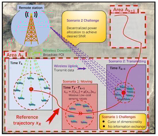
Figure 1. An illustration of the low-cost MWSN. At time $T_k$, the remote station wants to detect the area $A_k$, and therefore a reference trajectory is broadcast to a massive group of sensing robots. Then the robot team tracks the reference trajectory through decentralized optimal tracking control. When the area is fully detected, all sensing robots transmit the collected information back to the remote station. Then, a new area (reference trajectory) is broadcast once the data transmission is completed.

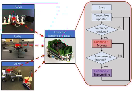
Figure 2. Low-cost mobile robots (e.g., AUVs, UAVs, and AGVs) have limited communication and computational resources. Hence, they alternate between two asynchronous modes: (1) Scenario 1—navigation; and (2) Scenario 2—data transmission. The workflow is illustrated in this figure.

4.1. Scenario 1: Optimal Navigation Formulation

Consider the motion dynamics of robot i in a team comprising N homogeneous robots as a stochastic differential equation:

$$\begin{array}{c}\hfill {\dot{x}}_{s,i}=\left[f\left(x_{s,i}\right)+g\left(x_{s,i}\right)u_{s,i}\right]dt+{\sigma }_{s}d{w}_{s,i},\end{array}$$

(1)

where $x_{s,i}$ and $u_{s,i}$ are smooth and Lipchitz nonlinear equations representing the agent’s states and motion control input, respectively. The functions $f\left(x_{s,i}\right)$ and $g\left(x_{s,i}\right)$ describe the robot’s motion dynamics. The term $w_{s,i}\left(t\right)$ denotes a set of independent Wiener processes representing environmental noise, while ${\sigma }_s$ is the constant diffusion matrix for these processes.

Next, at any time $T_k$, the tracking error can be represented as $e_{s,i}=x_{s,i}-A_k\left(t\right)$, where $A_k\left(t\right)$ is the current reference trajectory. The tracking error dynamics is thus derived as

$$\begin{array}{c}\hfill d{e}_{s,i}=d{x}_{s,i}-d{A}_k=[f_s\left(e_{s,i}\right)+g_s\left(e_{s,i}\right)u_{s,i}]dt+{\sigma }_{s}d{w}_{s,i},\end{array}$$

(2)

where $f_s\left(e_{s,i}\right)=f(e_{s,i}+A_k\left(t\right))-d{A}_k\left(t\right)/dt$, and $g_s\left(e_{s,i}\right)=g_i(e_{s,i}+A_k\left(t\right))$.

Remark 1.

The error dynamics in Equation (2) follow from the affine transformation $e_{s,i}=x_{s,i}-A_k\left(t\right)$. Since the Jacobian is the identity and the Hessian vanishes, Itô’s lemma reduces to $d{e}_{s,i}=d{x}_{s,i}-{\dot{A}}_k\left(t\right)dt$, with the extra term absorbed into $f_s(e_{s,i},t)$.

To track the reference trajectory in an optimal manner, a value function is proposed for any given time duration $[T_k,T^{\prime }]$ as follows:

$$\begin{array}{c}\hfill V_{s,i}(E,u_{s,i})=\mathbb{E}{\int }_{T_k}^{T^{\prime }}\left\{L_s(e_{s,i},u_{s,i})+{\mathrm{\Phi }}_s(e_{s,i},E)\right\}dt,\end{array}$$

(3)

where $E=[e_{s,1},\dots ,e_{s,N}]\in {\mathbb{R}}^{n\times N}$ is the augmented tracking error matrix including all agents. The motion energy and states value is defined as

$$\begin{array}{c}\hfill L_s(e_{s,i},u_{s,i})=\parallel e_{s,i}{\parallel }_{Q_s}^2+{\parallel u_{s,i}\parallel }_{R_s}^2,\end{array}$$

(4)

and the coupling function ${\mathrm{\Phi }}_s(e_{s,i},E):{\mathbb{R}}^{n\times N}\times {\mathbb{R}}^n\mapsto \mathbb{R}$ is an arbitrary Lipschitz function which represents the cost caused by other agents.

The value function (3) penalizes the tracking error, motion control input, and the coupling cost between other agents and local agent i. It is also worth noting that although the cost function summarizes the running cost over a finite time duration (i.e., $[T_{k-1},T_k]$), the problem is still an infinite time optimal control problem. Instead of a predefined value, the end time $T_k$ is determined by the time of all agents reaching the POI. Thus, the end time $T_k$ has no specific restriction applied. Another important assumption is that the time required for transmitting information is significantly less than the time for required moving, meaning that the transmitting time can be ignored when I consider the optimal tracking problem.

4.2. Scenario 2: Optimal Transmission Power Allocation Formulation

Next, the channel fading model is discussed. In wireless communication, the transmitted signal loss between the remote station and individual robot is related to the distance of the signal path [30,31]. Moreover, Ref. [32] shows that the power attenuation can be described as a stochastic differential equation (SDE) if the lognormal channel fading model is adopted. If we let the $x_R\in {\mathbb{R}}^n$ denote the position of the fixed remote station, then the distance between robot i and the remote station (i.e, transmitted path distance) can be represented as $e_{p,i}\left(t\right)=x_{s,i}-x_R$. Therefore, the dynamic equation of $e_{p,i}$ is derived as

$$\begin{array}{c}\hfill d{e}_{p,i}\left(t\right)=[f_p\left(e_{p,i}\right)+g_p\left(e_{p,i}\right)u_{s,i}]dt+{\sigma }_{s}d{w}_{s,i},\end{array}$$

(5)

where $f_p\left(e_{p,i}\right)=f(e_{p,i}+x_R)$ and $g_p\left(e_{p,i}\right)=g(e_{p,i}+x_R)$.

Letting ${\alpha }_i$ denote the power attenuation (loss) of the link between robot i and the remote station, this can be calculated by a function of the path distance ${\alpha }_i=exp(-e_{p,i}^T{e}_{p,i})$ [32]. Thus, the actual received power at the remote station is ${\alpha }_i{p}_i$. To guarantee the quality of service (QoS), which is measured by the signal-to-interference-plus-noise ratio (SINR), the transmitter’s power for individual robots needs to be coordinated. In other words, the consensus for transmission power needs to be achieved for all agents. According to related research [8,33,34,35,36], the SINR in a large population of users can be defined as

$$\begin{array}{c}\hfill {\xi }_i\left(t\right)={\displaystyle \frac{{\alpha }_i\left(t\right)p_i\left(t\right)}{I_i\left(t\right)+{\eta }_i}}={\displaystyle \frac{{\alpha }_i{p}_i}{{\sum }_{j\ne i}^N{\beta }_N{\alpha }_j{p}_j+{\eta }_i}},\end{array}$$

(6)

where $I_i$ is the interference and ${\eta }_i\ge 0$ denotes the variance power of the noise at its receiver node.

In (6), we approximate the aggregate interference coupling coefficient as ${\beta }_N\approx 1/N$. This assumption is not meant to describe all heterogeneous fading environments but serves as a tractable large-system surrogate that captures the dominant scaling behavior of interference with respect to the number of active users. When transmitters experience independent small-scale fading and random phases, the aggregate interference at a receiver can be modeled as a sum of N weakly correlated random variables. Under normalized transmitted power, each term contributes $O(1/N)$ to the total interference, and as N increases, the law of large numbers implies that the total interference remains bounded while the effective contribution of each interferer decays proportionally to $1/N$. This observation is consistent with shot-noise models of large wireless networks, where the interference field converges to a finite mean despite an increasing number of interferers [37,38]. In symmetric multi-user systems with homogeneous power control or scheduling, the interference power is effectively shared among N users, leading to an average cross-coupling that also scales inversely with N. Furthermore, the same approximation is adopted in other large-scale communication literatures such as [8].

The objective of communication QoS requires that the SINR is higher than or equal to a desired threshold, i.e., ${\xi }_i\ge {\mu }_i$. Meanwhile, the power allocation objective is to minimize the total power consumption for all users, i.e., $min{\sum }_{j=1}^N{p}_j$. Based on [8], the solution of the total power minimization subject to the QoS constraint is defined as

$$\begin{array}{c}\hfill {\displaystyle \frac{{\alpha }_i{p}_i}{{\sum }_{j\ne i}^N{\beta }_N{\alpha }_j{p}_j+{\eta }_i}}={\mu }_i>0,\end{array}$$

(7)

which is equivalent to

$$\begin{array}{cc}\hfill {\displaystyle \frac{{\alpha }_i{p}_i}{{\sum }_{j\ne i}{\beta }_N{\alpha }_j{p}_j+{\eta }_i}}& ={\mu }_i,\hfill \\ \hfill {\alpha }_i{p}_i& ={\mu }_i\left(\sum _{j\ne i}{\beta }_N{\alpha }_j{p}_j+{\eta }_i\right),\hfill \\ \hfill {\alpha }_i{p}_i& ={\mu }_i\left(\sum _{j=1}^N{\beta }_N{\alpha }_j{p}_j-{\beta }_N{\alpha }_i{p}_i+{\eta }_i\right),\hfill \\ \hfill {\alpha }_i{p}_i(1+{\mu }_i{\beta }_N)& ={\mu }_i\left(\sum _{j=1}^N{\beta }_N{\alpha }_j{p}_j+{\eta }_i\right),\hfill \\ \hfill {\displaystyle \frac{{\alpha }_i{p}_i}{{\sum }_{j=1}^N{\beta }_N{\alpha }_j{p}_j+{\eta }_i}}& ={\displaystyle \frac{{\mu }_i}{1+{\beta }_N{\mu }_i}}.\hfill \end{array}$$

(8)

With the assumption that $N\to \infty$, (8) can be calculated as

$$\begin{array}{c}\hfill \underset{N\to \infty }{lim}{\displaystyle \frac{{\alpha }_i{p}_i}{{\sum }_{j=1}^N{\beta }_N{\alpha }_j{p}_j+{\eta }_i}}=\underset{N\to \infty }{lim}{\displaystyle \frac{{\mu }_i}{1+{\beta }_N{\mu }_i}}={\mu }_i.\end{array}$$

(9)

Without loss of generality, the transmission power of the ith robot can be modeled and described similarly as in [8], i.e.,

$$\begin{array}{c}\hfill d{p}_i\left(t\right)=u_{p,i}dt+{\sigma }_{p}d{w}_{p,i},1\le i\le N,\end{array}$$

(10)

where $p_i$ represents the transmission power and $u_{p,i}\left(t\right)$ represents the power-control command generated by the base station or scheduler to regulate user i’s transmitted power in real time. In practice, this control corresponds to the standard closed-loop power-control signal used in modern systems (e.g., LTE or 5G NR), which adjusts the transmitted power at sub-millisecond intervals based on SINR feedback. The stochastic differential equation formulation serves as the continuous-time limit of this discrete process, where the drift term governed by $u_{p,i}$ models the deterministic adjustment of power and the diffusion term captures random channel fluctuations and measurement noise. This abstraction preserves the bounded, feedback-driven nature of practical power-control loops while enabling tractable stochastic analysis. Furthermore, ${\sigma }_{p}d{w}_{p,i}$ provides the random noise from the transmitter.

Therefore, the communication value function can be defined for each robot at time $T^{\prime }$ with transmitting time $T_x$ as

$$\begin{array}{c}\hfill V_{p,i}(\mathit{p},\mathit{\alpha },u_{p,i})=\mathbb{E}\left\{{\int }_{T^{\prime }}^{T^{\prime }+T_x}{\mathrm{\Phi }}_p(\mathit{p},\mathit{\alpha })+Q_p{p}_i^2+R_p{u}_{p,i}^2\right\}dt\end{array}$$

(11)

with

$$\begin{array}{c}\hfill {\mathrm{\Phi }}_p(\mathit{p},\mathit{\alpha })={\left[{\alpha }_i{p}_i-{\mu }_i\left({\beta }_N\sum _{j=1}^n{\alpha }_j{p}_j+{\eta }_i\right)\right]}^2,\end{array}$$

(12)

where $\mathit{p}$ and $\mathit{\alpha }$ represent the sets of all users’ power and the power loss of the ith agent, respectively, ${\mathrm{\Phi }}_p(·)$ is the coupling term that forces the transmitter to achieve the desired SINR, $R_p{u}_i^2$ represents the penalty of abrupt power adjustment, and $Q_p{p}_i^2$ represents the additional penalty of high power. Although the integration in (11) is to infinity, the transmission stops when the remote station receives all data.

The objective of an individual robot is to find the optimal control $u_{s,i}$ and $u_{p,i}$ such that the value functions (3) and (11) are minimized. It is easy to observe from (3) and (11) that the coupling terms ${\mathrm{\Phi }}_s(·)$ and ${\mathrm{\Phi }}_p(·)$ require the current information from other robots, which is unattainable. To overcome these difficulties, Mean Field Games are applied where coupling functions are replaced by a function that is related to the PDF of all agents’ state information.

5. Mean Field Type Control

Mean Field Game (MFG) theory [12] is an emerging technique that can effectively solve the stochastic decision-making and control problem with a large population of agents in a decentralized manner. In Mean Field Games, the information is encoded into a probability density function (PDF) which can be computed by a partial differential equation (PDE) named the Fokker–Planck–Kolmogorov (FPK) equation. The computed PDF overcomes the difficulty of collecting information from all other agents, as well as reducing the dimensions of the optimal control problem. In this section, the tasks in Scenarios 1 and 2 are formulated into two non-cooperative Mean Field Games. Then, a series of neural networks are designed and activated asynchronously to approximate the optimal solution. For example, when the robot is in Scenario 1, three NNs for Scenario 1 are activated, whereas Scenario 2’s NNs remain unchanged. The block diagram of the Actor–Critic–Mass (ACM) structure is demonstrated in Figure 3.

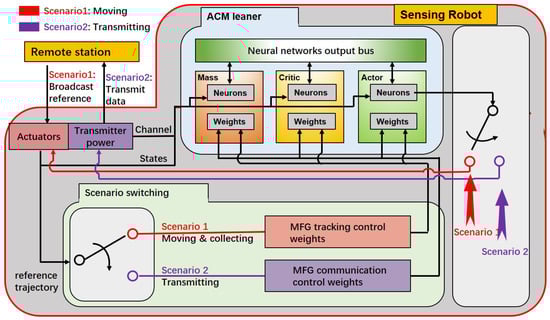
Figure 3. Block diagram of the Actor–Critic–Mass (ACM) architecture. Two sets of actor, critic, and mass neural networks are constructed to estimate the optimal control strategies for Scenario 1 and Scenario 2, respectively. These two sets are activated alternately based on the current scenario. Each neural network continuously interacts with the environment and updates its synaptic weights using real-time feedback, enabling online learning and adaptation.

5.1. Mean Field Power Allocation Games and Solution Learning

I first formulate Scenario 2 as a mean field type of transmission power allocation problem and derive the Actor–Critic–Mass structure to learn the optimal solution. As mentioned in the previous section, the coupling term ${\mathrm{\Phi }}_p(·)$ requires the current transmission power of other robots, which is unattainable. Therefore, I propose using the PDF to replace all agents’ transmission power $\mathit{p}$ and power loss $\mathit{\alpha }$.

Given a wireless channel, the PDFs of the power loss and transmission power for all robots, i.e., $\alpha \sim m_{\alpha }(\alpha ,t)$ and $p\sim m_p(p,t)$, are used to compute the joint PDF of the received power of the i-th robot, i.e., $m_g(\alpha ,p,t)$, with $\alpha p\in \mathrm{\Theta }=\left\{\alpha p\right|0\le \alpha p\le p_{max}\}$. Assuming $N\to \infty$, the SINR constraint can be replaced with the expected value as follows:

$$\begin{array}{c}\hfill {\mu }_i\left(t\right)={\displaystyle \frac{{\alpha }_i\left(t\right)p_i\left(t\right)}{\mathbb{E}\left(\alpha \left(t\right)p\left(t\right)\right)+{\eta }_i}}.\end{array}$$

(13)

While $m_p(p,t)$ changes, $m_{\alpha }(\alpha ,t)$ is fixed since the all agents remain still. Since the mobility and power allocation are separately considered, I consider the $\alpha$ and p as independent random variables and $\mathbb{E}\left[m_g(\alpha ,p,t)\right]=\mathbb{E}\left[m_{\alpha }(\alpha ,t)\right]\mathbb{E}\left[m_p(p,t)\right]$.

Then, the communication value function (11) can be changed accordingly as

$$\begin{array}{c}\hfill V_{p,i}(p_i,{\alpha }_i,u_{p,i},m_g,m_p)=\mathbb{E}{\int }_{T^{\prime }}^{\infty }\left\{{\mathrm{\Phi }}_p(p_i,{\alpha }_i,m_g,m_p)+Q_p{p}_i^2+R_p{u}_{p,i}^2\right\}dt\end{array}$$

(14)

with

$$\begin{array}{c}\hfill {\mathrm{\Phi }}_p(·)={\left[{\alpha }_i{p}_i-{\mu }_i\left(\mathbb{E}\left[m_{\alpha }(\alpha ,t)\right]\mathbb{E}\left[m_p(p,t)\right]+{\eta }_i\right)\right]}^2.\end{array}$$

(15)

To solve the optimal strategy which minimizes the value function, the HJB equation can be obtained. According to the optimal control theory [39], the HJB equation is given as

$$\begin{array}{c}\hfill 0=-{\partial }_t{V}_{p,i}(p_i,m_p,t)-{\displaystyle \frac{{\sigma }_p^2}{2}}{\partial }_{pp}{V}_{p,i}(p_i,m_p,t)H_p\left[p_i,{\partial }_p{V}_{p,i}(p_i,m_p,t)\right]-{\mathrm{\Phi }}_p(p_i,{\alpha }_i,m_g,m_p),\end{array}$$

(16)

where

$$H_p\left[p_i,{\partial }_p{V}_{p,i}(p_i,m_p,t)\right]=Q_p{p}_i^2+R_p{u}_{+}^2{\partial }_p{V}_{p,i}(p_i,m_p,t)u_{p,i}.$$

(17)

The optimal power adjustment strategy for individual agents can be represented as

$$\begin{array}{c}\hfill u_i^{*}(p_i,u_{p,i},m_p)=-{\displaystyle \frac{1}{2}}{R}_p^{-1}{\partial }_p{V}_{p,i}^{*}(p_i,u_{p,i},m_p)\end{array}$$

(18)

To solve the HJB, i.e., Equation (16), the attenuation mass distribution $m_{\alpha }(\alpha ,t)$ and the transmission power mass distribution $m_p(p,t)$ are needed. Recalling the Mean Field Game (MFG) [13], the probability density function (PDF) $m_p(p,t)$ can be attained by solving the FPK equation:

$$\begin{array}{cc}\hfill & 0={\partial }_t{m}_p(p,t)-{\displaystyle \frac{{\sigma }_p^2}{2}}{\partial }_{pp}{m}_p(p_i,t)+{\partial }_p\left[u_{p,i}{m}_p(p,t)\right]\hfill \\ \hfill & m_p(p,0)=m_{p,0}\left(p\right).\hfill \end{array}$$

(19)

The expected value $\mathbb{E}\left[m_{\alpha }(\alpha ,t)\right]$ can be calculated by substituting the monotonic power attenuation function ${\alpha }_i=exp(-e_{p,i}^T{e}_{p,i})$. Furthermore, the PDF of the transmitted path loss $e_{p,i}$ in (5), $m_g$, can also be solved by the following FPK equation:

$$\begin{array}{cc}\hfill & {\partial }_t{m}_g(e_p,t)+{\displaystyle \frac{{\sigma }_s^2}{2}}\Delta m_g(e_p,t)-div\left[m_g\left(f_p\left(e_{p,i}\right)+g_p\left(e_{p,i}\right)u_{s,i}\right)\right]=0\hfill \\ \hfill & m_g(e_p,0)=m_{g}0\left(e_p\right),\hfill \end{array}$$

(20)

where $u_{s,i}$ is the motion control of the robot that is known in Scenario 2 and $m_{g}0\left(e_p\right)$ is the initial transmitted path loss distribution.

Finally, the optimal strategy based on a Mean Field Game for all agents is officially defined. Considering the aforementioned value function (14), the optimization of the transmission power allocation for N players, i.e., Scenario 2, can be formulated as a non-cooperative game.

In Scenario 2, each mobile sensing robot (player) tries to minimize the value function given in (14) by computing a dynamic transmission power adjustment rate $u_{p,i}$. Since the coupling effect is considered in the value function, the Nash Equilibrium is the optimal strategy for individual agents, while the number of agents is infinite. Let ${\Omega }_p\left(t\right)=\{u_{p,1}\left(t\right),\cdots ,u_{p,1}\left(t\right)\}\in {\mathbb{R}}^N$ denote the set of transmission power for all mobile sensing robots at time t. Define a mapping ${\mathbb{F}}_p:(\mathit{p}\left(t\right),{\Omega }_p\left(t\right))\to u_{p,i}\left(t\right)$ to represent the power adjustment strategy set for agent i. I further denote ${\mathcal{U}}_{p,-i}$ as the set of transmission power other than that for agent i. Then, the optimal strategy equilibrium, i.e., the ${ϵ}_N$ Nash Equilibrium, can be defined as follows.

Definition 1 (${ϵ}_N$ Nash Equilibrium (NE) of Scenario 2).

Given power set $\mathit{p}\left(t\right)$ and action set ${\Omega }_p\left(t\right)$ at any time t, the ${ϵ}_N$ Nash Equilibrium (NE) of the N-player non-cooperative power allocation game is a strategy set ${\Omega }_s^{*}=(u_{p,1}^{*},\cdots ,u_{p,N}^{*})$ that is generated by $u_{p,i}^{*}={\mathbb{F}}_p(\mathit{p}\left(t\right),{\Omega }_p\left(t\right))$ and satisfies the following conditions:

$$\begin{array}{c}\hfill V_{p,i}(E,u_{p,i}^{*})\le V_{p,i}(\mathit{p}\left(t\right),u_{p,i})+{ϵ}_N,\forall u_{p,i}\in {\mathcal{U}}_p\setminus u_{p,i}^{*},i=1,2,3,\cdots ,N,\end{array}$$

(21)

where ${ϵ}_N>0$.

According to recent studies [15,40], the solution to the coupled Hamilton–Jacobi-Bellman (HJB) and Fokker–Planck–Kolmogorov (FPK) equations yields an ${ϵ}_N$-Nash equilibrium, where ${lim}_{N\to \infty }{ϵ}_N=0$.

Remark 2.

Unlike conventional distributed control methods, which require precise real-time information from neighboring agents, the Mean Field Game (MFG)-based decentralized control framework allows each agent to make decisions based on local information and the aggregate effect of the entire multi-agent system (MAS). This aggregate influence is captured through the probability density function (PDF) of agents’ transmission powers, denoted by $m_p(p,t)$. Notably, this PDF can be computed using the FPK equation [12], without requiring direct access to other agents’ instantaneous states or actions.

To determine the optimal transmission power, one must simultaneously solve the coupled Hamilton–Jacobi–Bellman (HJB) and Fokker–Planck–Kolmogorov (FPK) equations. However, this is inherently challenging: the HJB equation, i.e., Equation (16), is a backward-in-time partial differential equation (PDE), whereas the FPK equation, Equation (19), evolves forward in time. This opposing temporal structure makes the real-time solution of the mean field design highly complex.

To address this challenge, a novel online adaptive reinforcement learning framework, termed the Actor–Critic–Mass (ACM) architecture, is proposed. In this framework, three neural networks—the actor, the critic, and the mass network—are constructed to approximate the solutions to Equation (18), Equation (16), and Equation (19), respectively.

Assuming ideal neural network weights $W_{V,p,i}^T$, $W_{u,p,i}^T$, and $W_{m,p,i}^T$, respectively, the optimal value function, control policy, and mass distribution can be approximated as follows:

$$\begin{array}{c}\hfill \left\{\begin{array}{cc}\hfill V_{p,i}^{*}(p_i,m_p,t)& =W_{V,p,i}^T{\varphi }_{V,p,i}\left(p_i\left(t\right)\right)+{\epsilon }_{V,p,i},\hfill \\ \hfill u_{p,i}^{*}(p_i,m_p)& =W_{u,p,i}^T{\varphi }_{u,p,i}\left(p_i\left(t\right)\right)+{\epsilon }_{u,p,i},\hfill \\ \hfill m_p(p_i,t)& =W_{m,p,i}^T{\varphi }_{m,p,i}\left(p_i\left(t\right)\right)+{\epsilon }_{m,p,i},\hfill \end{array}\right.\end{array}$$

(22)

where ${\varphi }_{V,p,i}\left(p_i\left(t\right)\right)$, ${\varphi }_{u,p,i}\left(p_i\left(t\right)\right)$, and ${\varphi }_{m,p,i}\left(p_i\left(t\right)\right)$ are bounded, continuous activation functions, and ${\epsilon }_{V,p,i}$, ${\epsilon }_{u,p,i}$, and ${\epsilon }_{m,p,i}$ denote the neural network approximation errors.

Correspondingly, the learned approximations for the value function, power control strategy, and mass distribution are expressed as

$$\begin{array}{c}\hfill \left\{\begin{array}{cc}\hfill {\widehat{V}}_{p,i}(p_i,{\widehat{m}}_{p,i},t)& ={\widehat{W}}_{V,p,i}^T{\widehat{\varphi }}_{V,p,i},\hfill \\ \hfill {\widehat{u}}_{p,i}(p_i,{\widehat{m}}_{p,i})& ={\widehat{W}}_{u,p,i}^T{\widehat{\varphi }}_{u,p,i},\hfill \\ \hfill {\widehat{m}}_{p,i}(p_i,t)& ={\widehat{W}}_{m,p,i}^T{\widehat{\varphi }}_{m,p,i},\hfill \end{array}\right.\end{array}$$

(23)

where ${\widehat{\varphi }}_{V,p,i}$, ${\widehat{\varphi }}_{u,p,i}$, and ${\widehat{\varphi }}_{m,p,i}$ represent the online-estimated basis functions corresponding to each approximated quantity.

Substituting the neural network approximations in Equation (23) into the original HJB equation (16), the optimal control law (18), and the FPK equation (19), the equations no longer hold exactly. Instead, residual errors are introduced, which are then used to update the critic, actor, and mass networks over time. These residuals are defined as follows:

$$\begin{array}{cc}\hfill e_{HJB,p,i}& =-{\partial }_t{\widehat{V}}_{p,i}(p_i,{\widehat{m}}_{p,i},t)-{\mathrm{\Phi }}_p(p_i,{\alpha }_i,{\widehat{m}}_{g,i},m_{p,i})\hfill \\ & \hfill -{\displaystyle \frac{{\sigma }_p^2}{2}}{\partial }_{pp}{\widehat{V}}_{p,i}(p_i,{\widehat{m}}_{p,i},t)H_p\left[p_i,{\partial }_p{\widehat{V}}_{p,i}\right]\hfill \end{array}$$

(24)

$$e_{FPK,p,i}={\partial }_t{\widehat{m}}_{p,i}(p,t)-{\displaystyle \frac{{\sigma }_p^2}{2}}{\partial }_{pp}{\widehat{m}}_{p,i}(p_i,t)+{\partial }_p\left[{\widehat{u}}_{p,i}{\widehat{m}}_{p,i}\right]$$

(25)

$$e_{u,p,i}=-{\displaystyle \frac{1}{2}}{R}_p^{-1}{\partial }_p{\widehat{V}}_{p,i}(p_i,{\widehat{m}}_{p,i},t)$$

(26)

The residual terms in Equations (24)–(26) are obtained by substituting the neural network approximations into the original HJB, FPK, and optimal control equations, respectively, and represent the resulting approximation errors when these equations are not exactly satisfied.

According to Equation (22), these approximation errors vanish when the ideal neural network weights are reached. Hence, a gradient descent-based update law is applied to minimize the residuals and iteratively learn the optimal weights in Equation (22):

$$\begin{array}{cccc}\hfill & \mathbf{Critic}:\hfill & \hfill & {\dot{\widehat{W}}}_{V,p,i}=-{\alpha }_{h,p,i}{\nabla }_{W_{V,p,i}}{e}_{HJB,p,i}\hfill \end{array}$$

(27)

$$\begin{array}{cccc}\hfill & \mathbf{Mass}:\hfill & \hfill & {\dot{\widehat{W}}}_{m,p,i}=-{\alpha }_{m,p,i}{\nabla }_{W_{m,p,i}}{e}_{FPK,p,i}\hfill \end{array}$$

(28)

$$\begin{array}{cccc}\hfill & \mathbf{Actor}:\hfill & \hfill & {\dot{\widehat{W}}}_{u,p,i}=-{\alpha }_{u,p,i}{\nabla }_{W_{u,p,i}}{e}_{u,p,i}\hfill \end{array}$$

(29)

where ${\alpha }_{h,p,i}$, ${\alpha }_{m,p,i}$, and ${\alpha }_{u,p,i}$ denote the learning rates for the critic, mass, and actor networks, respectively.

5.2. Mean Field Optimal Navigation Games

As shown in [10], the decentralized navigation problem for large-scale mobile sensor networks can be formulated as a mean-field-type optimal tracking control problem. Let $m_s(e_s,t)$ denote the time-varying probability density function (PDF) of the agents’ tracking errors at time t. It is assumed that the coupling function ${\mathrm{\Phi }}_s(e_{s,i},E)$ depends on the distribution of tracking errors and can be expressed as ${\mathrm{\Phi }}_s(e_{s,i},m_s(e_{s,i},t))$. With this, the cost function in Equation (3) becomes

$$\begin{array}{c}\hfill V_{s,i}(e_{s,i},m_s,u_{s,i})=\mathbb{E}{\int }_{T_k}^{T^{\prime }}\left[L_s(e_{s,i},u_{s,i})+{\mathrm{\Phi }}_s(e_{s,i},m_s)\right]dt.\end{array}$$

(30)

To minimize this cost, the corresponding Hamilton–Jacobi–Bellman (HJB) equation can be derived as in [10]:

$$\begin{array}{c}\hfill 0=-{\partial }_t{V}_{s,i}(e_{s,i},m_s,t)-{\displaystyle \frac{{\sigma }_s^2}{2}}\Delta V_{s,i}(e_{s,i},m_s,t)+H_s\left[e_{s,i},{\partial }_{e_s}{V}_{s,i}(e_{s,i},m_s,t)\right]-{\mathrm{\Phi }}_s(e_{s,i},m_s),\end{array}$$

(31)

where the Hamiltonian $H_s(·)$ is given by

$$\begin{array}{c}\hfill H_s\left[e_{s,i},{\partial }_{e_s}{V}_{s,i}\right]=e_{s,i}^{\top }{Q}_s{e}_{s,i}+u_{s,i}^{\top }{R}_s{u}_{s,i}+{\partial }_{e_s}{V}_{s,i}^{\top }\left[f_s\left(e_{s,i}\right)+g_s\left(e_{s,i}\right)u_{s,i}\right].\end{array}$$

(32)

Solving the HJB equation yields the optimal cost-to-go function and control policy. The optimal control input is given by

$$\begin{array}{c}\hfill u_{s,i}^{*}\left(e_{s,i}\right)=-{\displaystyle \frac{1}{2}}{R}_s^{-1}{g}_s^{\top }\left(e_{s,i}\right){\partial }_{e_{s,i}}{V}_{s,i}^{*}(e_{s,i},m_s,t).\end{array}$$

(33)

Meanwhile, the tracking error distribution $m_s(e_s,t)$ evolves according to the Fokker–Planck–Kolmogorov (FPK) equation:

$$\begin{array}{cc}\hfill & 0={\partial }_t{m}_s(e_{s,i},t)-{\displaystyle \frac{{\sigma }_s^2}{2}}\Delta m_s(e_{s,i},t)-\nabla ·\left(m_s{D}_p{H}_s\left[e_{s,i},{\partial }_{e_{s,i}}{V}_{s,i}(e_{s,i},m_s,t)\right]\right),\hfill \\ \hfill & m_s(e_s,0)=m_{s,0}\left(e_s\right),\hfill \end{array}$$

(34)

where $D_p$ denotes differentiation with respect to the second argument. Solving the coupled HJB–FPK equations yields the ${ϵ}_N$-Nash equilibrium for Scenario 1.

To avoid solving the coupled PDEs directly, I employ a mean field reinforcement learning approach to approximate the optimal value function, control policy, and distribution. These are represented using neural networks as follows:

$$\begin{array}{c}\hfill \left\{\begin{array}{cc}\hfill {\widehat{V}}_{s,i}(e_{s,i},m_s,t)& ={\widehat{W}}_{V,s,i}^{\top }{\widehat{\varphi }}_{V,s,i},\hfill \\ \hfill {\widehat{u}}_{s,i}(e_{s,i},m_s)& ={\widehat{W}}_{u,s,i}^{\top }{\widehat{\varphi }}_{u,s,i},\hfill \\ \hfill {\widehat{m}}_{s,i}(e_s,t)& ={\widehat{W}}_{m,s,i}^{\top }{\widehat{\varphi }}_{m,s,i}\hfill \end{array}\right.\end{array}$$

(35)

The weights of the neural networks are updated via gradient descent using the residual errors from the HJB, FPK, and control equations:

$$\begin{array}{cc}\hfill \mathbf{Critic}:& {\dot{\widehat{W}}}_{V,s,i}=-{\alpha }_{h,s,i}{\nabla }_{W_{V,s,i}}{e}_{HJB,s,i}\hfill \end{array}$$

(36)

$$\begin{array}{cc}\hfill \mathbf{Mass}:& {\dot{\widehat{W}}}_{m,s,i}=-{\alpha }_{m,s,i}{\nabla }_{W_{m,s,i}}{e}_{FPK,s,i}\hfill \end{array}$$

(37)

$$\begin{array}{cc}\hfill \mathbf{Actor}:& {\dot{\widehat{W}}}_{u,s,i}=-{\alpha }_{u,s,i}{\nabla }_{W_{u,s,i}}{e}_{u,s,i}\hfill \end{array}$$

(38)

Here, $e_{HJB,s,i}$, $e_{FPK,s,i}$, and $e_{u,s,i}$ denote the residual errors derived from the HJB Equation (31), the FPK Equation (34), and the control policy (33), respectively.

5.3. Convergence of Neural Network Weights

To ensure the reliability of the proposed learning framework, it is essential to analyze the convergence properties of the neural networks. Given the structural similarity between the neural networks used in Scenario 1 and Scenario 2, I focus our analysis on Scenario 2 without loss of generality.

Recall the update laws defined in Equations (27)–(29). The weight estimation errors of the actor, critic, and mass networks can be expressed as

$$\begin{array}{cc}\hfill & \mathbf{Critic}\mathbf{NN}:{\dot{\tilde{W}}}_{V,p,i}\left(t\right)=-{\dot{\widehat{W}}}_{V,p,i}\left(t\right)\hfill \end{array}$$

(39)

$$\begin{array}{cc}\hfill & \mathbf{Mass}\mathbf{NN}:{\dot{\tilde{W}}}_{m,p,i}\left(t\right)=-{\dot{\widehat{W}}}_{m,p,i}\left(t\right)\hfill \end{array}$$

(40)

$$\begin{array}{cc}\hfill & \mathbf{Actor}\mathbf{NN}:{\dot{\tilde{W}}}_{u,p,i}\left(t\right)=-{\dot{\widehat{W}}}_{u,p,i}\left(t\right)\hfill \end{array}$$

(41)

where the weight estimation error is defined as $\tilde{W}=W-\widehat{W}$, with ${\tilde{W}}_{V,p,i}$, ${\tilde{W}}_{m,p,i}$, and ${\tilde{W}}_{u,p,i}$ representing the respective errors for the critic, mass, and actor networks.

Firstly, a lemma regarding the closed-loop dynamics is proposed.

Lemma 1.

Consider the continuous-time system described by Equation (10). There exists an optimal mean field-type control input $u_{p,i}^{*}$ such that the resulting closed-loop system dynamics,

$$\begin{array}{c}\hfill u_{p,i}^{*}+{\sigma }_p{\displaystyle \frac{d{w}_{p,i}}{dt}},\forall 0<i\le N,\end{array}$$

(42)

satisfy the inequality

$$\begin{array}{c}\hfill p_i\left[u_{p,i}^{*}+{\sigma }_p{\displaystyle \frac{d{w}_{p,i}}{dt}}\right]\le -\gamma {∥p_i∥}^2,\end{array}$$

(43)

where $\gamma >0$ is a positive constant.

Based on this lemma, the performance of the Actor–Critic–Mass (ACM) learning algorithm in Scenario 2 can be analyzed through the following theorem.

Theorem 1 (Closed-loop Stability).

Let the initial control input be admissible, and suppose the actor, critic, and mass neural network weights are initialized within a compact set. Assume the neural network weight update laws are given by Equations (27)–(29). Then, there exist the positive constants ${\alpha }_{h,p,i}$, ${\alpha }_{m,p,i}$, and ${\alpha }_{u,p,i}$ such that the transmission power $p_i$ and the weight estimation errors ${\tilde{W}}_{V,p,i}$, ${\tilde{W}}_{m,p,i}$, and ${\tilde{W}}_{u,p,i}$ of the critic, mass, and actor networks, respectively, are all uniformly ultimately bounded (UUB). Moreover, the estimated value function ${\widehat{V}}_{p,i}$, mass function ${\widehat{m}}_{p,i}$, and control input ${\widehat{u}}_{p,i}$ are also UUB. If the neural networks are sufficiently expressive (i.e., with enough neurons and a properly designed architecture), the reconstruction errors can be made arbitrarily small. Under such ideal conditions, the system state $p_i$ and the weight estimation errors ${\tilde{W}}_{V,p,i}\left(t\right)$, ${\tilde{W}}_{m,p,i}\left(t\right)$, and ${\tilde{W}}_{u,p,i}\left(t\right)$ will asymptotically converge to zero, ensuring asymptotic stability of the closed-loop system.

Proof. 

A brief proof sketch is provided: Consider the transmission power dynamics in Equation (10) and the neural network approximations in Equation (23). Let the ideal network weights be $W_{V,p,i}$, $W_{u,p,i}$, and $W_{m,p,i}$, and their online estimates be ${\widehat{W}}_{V,p,i}$, ${\widehat{W}}_{u,p,i}$, and ${\widehat{W}}_{m,p,i}$. Define the corresponding weight estimation errors as ${\tilde{W}}_{V,p,i}=W_{V,p,i}-{\widehat{W}}_{V,p,i}$, ${\tilde{W}}_{u,p,i}=W_{u,p,i}-{\widehat{W}}_{u,p,i}$, and ${\tilde{W}}_{m,p,i}=W_{m,p,i}-{\widehat{W}}_{m,p,i}$. The residual errors $e_{HJB,p,i}$, $e_{FPK,p,i}$, and $e_{u,p,i}$ are defined in Equations (24)–(26) as the deviations obtained when the approximated neural networks are substituted into the corresponding Hamilton–Jacobi–Bellman (HJB), Fokker–Planck–Kolmogorov (FPK), and optimal control equations, respectively. The update laws in Equations (27)–(29) minimize these residuals through gradient descent with learning rates ${\alpha }_{h,p,i}$, ${\alpha }_{m,p,i}$, and ${\alpha }_{u,p,i}$. To analyze convergence, consider the following Lyapunov candidate function:

$$\mathcal{L}=c_1{p}_i^2+\frac{1}{2}{\tilde{W}}_{V,p,i}^{\top }{\tilde{W}}_{V,p,i}+\frac{1}{2}{\tilde{W}}_{u,p,i}^{\top }{\tilde{W}}_{u,p,i}+\frac{1}{2}{\tilde{W}}_{m,p,i}^{\top }{\tilde{W}}_{m,p,i},$$

where $c_1>0$ is a constant and $p_i$ is the transmission power of agent i. Differentiating $\mathcal{L}$ along the trajectories of the closed-loop system and substituting the learning laws (27)–(29) yields

$$\dot{\mathcal{L}}\le -\underline{\lambda }{p}_i^2-{\alpha }_{h,p,i}\parallel {\nabla }_{{\widehat{W}}_{V,p,i}}{e}_{HJB,p,i}{\parallel }^2-{\alpha }_{u,p,i}\parallel {\nabla }_{{\widehat{W}}_{u,p,i}}{e}_{u,p,i}{\parallel }^2-{\alpha }_{m,p,i}\parallel {\nabla }_{{\widehat{W}}_{m,p,i}}{e}_{FPK,p,i}{\parallel }^2+C\parallel \epsilon \parallel ,$$

where $\underline{\lambda },C>0$ are constants and $\epsilon$ denotes the bounded neural network approximation errors introduced in Equation (22). The inequality shows that $\dot{\mathcal{L}}$ is negative definite up to a small residual term proportional to $\parallel \epsilon \parallel$, implying that both the transmission power $p_i$ and the weight estimation errors remain uniformly ultimately bounded (UUB). Under the standard universal approximation theorem, if the neural networks are sufficiently expressive such that the approximation errors $\epsilon$ can be made arbitrarily small, then $\dot{\mathcal{L}}<0$ and the system trajectories asymptotically converge to the optimal solution $(V_{p,i}^{★},u_{p,i}^{★},m_{p,i}^{★})$. This establishes the stability and convergence results stated in Theorem 1.    □

The performance for the mean field navigation game can be similarly obtained. Furthermore, the algorithm can be summarized as a pseudocode in Algorithm 1.

Algorithm 1 ACM for Mean Field Navigation (Scenario 1) and Power Control (Scenario 2)

Require: Dynamics $f_s,g_s$, diffusivities ${\sigma }_s,{\sigma }_p$, costs $(Q_s,R_s),(Q_p,R_p)$, schedule $\mathcal{C}\left(t\right)$, stepsizes ${\alpha }_h,{\alpha }_m,{\alpha }_u$ 1: Initialize weights $({\widehat{W}}_{V,1},{\widehat{W}}_{u,1},{\widehat{W}}_{m,1})$ and $({\widehat{W}}_{V,2},{\widehat{W}}_{u,2},{\widehat{W}}_{m,2})$ 2: Define ${\Sigma }_1\leftarrow {\sigma }_s{\sigma }_s^T$, ${\Sigma }_2\leftarrow {\sigma }_p^2$ 3: for $t=0,1,\dots ,T-1$ do 4:         $c\leftarrow \mathcal{C}\left(t\right)$            ▹$c=s$ navigation, $c=2$ communication 5:         if $c=1$ then 6:          ${\xi }_t\leftarrow e_t=x_t-A_k\left(t\right)$,   $G\leftarrow g_s\left(e_t\right)$,   $\mathrm{\Phi }({\xi }_t,\widehat{m})\leftarrow {\mathrm{\Phi }}_s(e_t,{\widehat{m}}_s)$,   $\Sigma \leftarrow {\Sigma }_1$ 7:         else 8:          ${\xi }_t\leftarrow p_t$,   $G\leftarrow I$,   $\mathrm{\Phi }({\xi }_t,\widehat{m})\leftarrow {\mathrm{\Phi }}_p(p_t,{\alpha }_t,\widehat{m})$,   $\Sigma \leftarrow {\Sigma }_2$ 9:         end if 10:       Mass step (FPK residual): 11:       ${\widehat{m}}_c(·,t)\leftarrow {\mathrm{MassNN}}_c({\xi }_t,t)$;    ${\widehat{m}}_c\leftarrow \mathrm{Normalize}\left(\mathrm{softplus}\left({\widehat{m}}_c\right)\right)$ 12:       $e_{\mathrm{FPK}}\leftarrow {\partial }_t{\widehat{m}}_c-\frac{1}{2}\nabla ·(\Sigma \nabla {\widehat{m}}_c)+\nabla ·\left({\widehat{u}}_c{\widehat{m}}_c\right)$ 13:       ${\widehat{W}}_{m,c}\leftarrow {\widehat{W}}_{m,c}-{\alpha }_m{\nabla }_{{\widehat{W}}_{m,c}}{\parallel e_{\mathrm{FPK}}\parallel }^2$ 14:       Critic step (HJB residual): 15:       ${\widehat{V}}_c\leftarrow {\mathrm{CriticNN}}_c({\xi }_t,t,{\widehat{m}}_c)$;   $g_V\leftarrow {\nabla }_{\xi }{\widehat{V}}_c$;   $H\leftarrow$            $\left\{\begin{array}{cc}{\xi }_t^T{Q}_c{\xi }_t+u_t^T{R}_c{u}_t+g_V^T\left[f_c\left({\xi }_t\right)+G{u}_t\right],\hfill & s=1\hfill \\ Q_p{p}_t^2+R_p{u}_t^2+g_V^T{u}_t,\hfill & s=2\end{array}\right.$ 16:       $e_{\mathrm{HJB}}\leftarrow -{\partial }_t{\widehat{V}}_c-\frac{1}{2}\mathrm{tr}(\Sigma {\nabla }_{\xi }^2{\widehat{V}}_c)+H-\mathrm{\Phi }({\xi }_t,{\widehat{m}}_c)$ 17:       ${\widehat{W}}_{V,c}\leftarrow {\widehat{W}}_{V,c}-{\alpha }_h{\nabla }_{{\widehat{W}}_{V,c}}{\parallel e_{\mathrm{HJB}}\parallel }^2$ 18:       Actor step (policy residual): 19:       $u_t\leftarrow {\mathrm{ActorNN}}_c({\xi }_t,{\widehat{m}}_c)$ 20:       $r_u\leftarrow \left\{\begin{array}{cc}{u}_t+\frac{1}{2}{R}_c^{-1}{G}^T{g}_V,\hfill & s=1\hfill \\ u_t+\frac{1}{2}{R}_p^{-1}{g}_V,\hfill & s=2\end{array}\right.$ 21:       ${\widehat{W}}_{u,c}\leftarrow {\widehat{W}}_{u,c}-{\alpha }_u{\nabla }_{{\widehat{W}}_{u,c}}{\parallel r_u\parallel }^2$ 22:       Apply $u_t$ to environment, step to $(t+1)$, log instantaneous cost 23: end for

6. Simulations

To validate the effectiveness of the proposed Actor–Critic–Mass (ACM) algorithm and its scalability in large-scale mobile wireless sensor networks, a series of numerical simulations are conducted. The simulations are designed to evaluate both navigation and communication performance under decentralized control. Specifically, the tracking accuracy, convergence of the mean field learning process, and communication quality of service (QoS) compared with a baseline decentralized algorithm are analyzed. The following subsections describe the simulation setup, performance metrics, and comparative results in detail.

Simulation Setup

The performance of the proposed decentralized multi-agent reinforcement learning algorithm is evaluated using a network of 1000 mobile wireless sensors. The simulation is conducted within a 6 × 5 m² workspace. All agents are randomly initialized within this area, and a remote station is located at the origin.

The mobile sensors are tasked with tracking four distinct trajectories corresponding to four areas of interest. Each trajectory $A_k\left(t\right)$, for $k=1,2,3,4$, is defined as

$$\begin{array}{cc}\hfill A_1\left(t\right)& =\left[\begin{array}{c}0.4sin(2t-2T_1)+13\\ 0.1t-0.1T_1+1.7\end{array}\right],A_2\left(t\right)=\left[\begin{array}{c}0.5sin(2t-2T_2)+0.05t-0.05T_2+2.5\\ 0.1t-0.1T_2+1.5\end{array}\right],\hfill \end{array}$$

(44)

$$\begin{array}{cc}\hfill A_3\left(t\right)& =\left[\begin{array}{c}0.1t-0.1T_3+2.5\\ 0.4sin(2t-2T_3)+1\end{array}\right],A_4\left(t\right)=\left[\begin{array}{c}0.1t-0.1T_4+1.1\\ 0.4sin(2t-2T_4)-0.03t+0.03T_4+1.7\end{array}\right],\hfill \end{array}$$

(45)

where $T_k$ denotes the activation time for trajectory k.

Each mobile sensor spends 20 s navigating along each reference trajectory. After completing the navigation for one area, the agent spends 15 s transmitting its collected data back to the remote station. The overall simulation timeline is illustrated in Figure 4, where $A_k$ denotes the tracking phase for area k and $P_k$ denotes the corresponding data transmission phase.

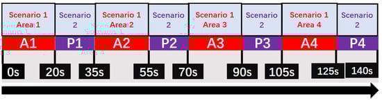
Figure 4. Timeline of scenarios. $P1$ stands for transmission location 1, and so on.

The desired transmission SINR is set to $0.6$, and the noise variance for all agents is $\eta =0.1$. The diffusion coefficients are set as ${\sigma }_s=0.1I_2$ and ${\sigma }_p=0.2I_2$. The cost function parameters are chosen as $Q_s=15I_2$, $Q_p=1$, $R_s=I_2$, and $R_p=1$. The mean field coupling function from Equation (30) is defined as

$$\begin{array}{c}\hfill {\mathrm{\Phi }}_s(m_s,e_{s,i},t)={∥e_{s,i}\left(t\right)-\mathbb{E}\left[m_s(e,t)\right]∥}^2.\end{array}$$

(46)

The initial distribution of agents’ positions is modeled as a Gaussian:

$$\begin{array}{c}\hfill m_{s,0}\sim \mathcal{N}\left(\left[\begin{array}{c}0.25\\ 0.25\end{array}\right],\left[\begin{array}{cc}0.3^2& 0\\ 0& 0.3^2\end{array}\right]\right).\end{array}$$

(47)

The simulation parameters are summarized in Table 1. A flow chart of the simulation process is provided in Figure 5. The actor, critic, and mass neural networks for both scenarios are updated separately. As shown, each agent starts by operating individually and alternates between the navigation and communication phases. In the navigation phase, the agent observes its state $x_{s,i}$, estimates the population distribution $m_s$ by solving the Fokker–Planck–Kolmogorov (FPK) equation, and computes the value function $V_s$ from the Hamilton–Jacobi–Bellman (HJB) equation. A new optimal control action $u_s$ is then generated and implemented to update the agent’s trajectory. Similarly, in the communication phase, the agent observes its relative distance $e_{s,i}$ to the remote station, updates the power distribution $m_g$ via the FPK equation, and evaluates the value function $V_p$ using the HJB equation to produce the optimal transmission power $u_p$. The new actions from both phases are implemented iteratively, allowing each agent to adapt its motion and power in real time until convergence to the mean field equilibrium occurs.

Table 1. Simulation parameters.

Parameter	Value
N	1000
Workspace size	$6\mathrm{m}\times 5\mathrm{m}$
$x_R$	$(0,0)$
$T_{\mathrm{nav}}$	$20\mathrm{s}$
$T_{\mathrm{tx}}$	$15\mathrm{s}$
$\mu$	$0.6$
$\eta$	$0.1$
${\sigma }_s$	$0.1I_2$
${\sigma }_p$	$0.2I_2$
$Q_s$	$15I_2$
$R_s$	$I_2$
$Q_p$	1
$R_p$	1
${\mathrm{\Phi }}_s(e_s,m_s)$	$\parallel e_s-\mathbb{E}\left[m_s\right]{\parallel }^2$
$m_{s,0}$	$\mathcal{N}\left(\left[\begin{array}{c}0.25\\ 0.25\end{array}\right],\left[\begin{array}{cc}0.32& 0\\ 0& 0.32\end{array}\right]\right)$
$\Delta t$	$0.05\mathrm{s}$
Neural network type	2 hidden layers, 64 neurons, ReLU
Learning rates $({\alpha }_{h,p,i},{\alpha }_{m,p,i},{\alpha }_{u,p,i})$	$({10}^{-3},{10}^{-3},5\times {10}^{-4})$

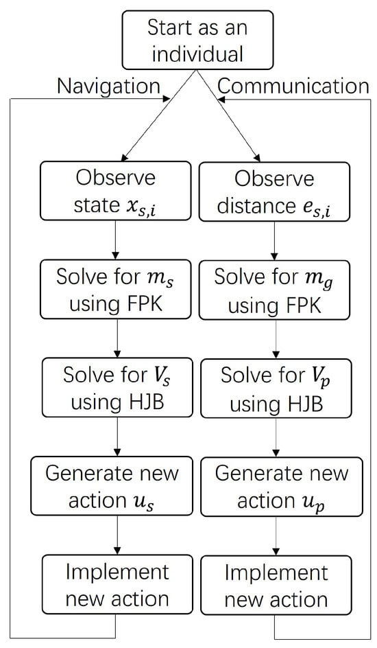
Figure 5. The flow chart of the algorithm.

To approximate the solutions of the HJB equations [Equations (31) and (16)], the FPK equations [Equations (34) and (19)], and the optimal control policies $u_{s,i}$ and $u_{p,i}$, I design and deploy three neural networks: Critic NN, Mass NN, and Actor NN.

Figure 6 illustrates the trajectories of all mobile sensors throughout the simulation. The blue curves represent the desired reference trajectories, while the data transmission points are indicated by red squares. The thin colored curves correspond to the individual trajectories of the 1000 mobile sensing agents. It can be clearly observed that the agents successfully track the desired paths with high accuracy. The detailed tracking error average and the percentage are included in Table 2. On average, the four areas achieved $2.32\%$ accuracy at the end of each stage.

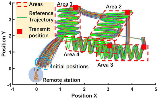
Figure 6. The overall trajectory for all sensing robots in Scenario 1. The red squares represent the transmitting points. The green curve represents the tracking reference.

Table 2. Trajectory tracking errors by time.

Area	Time	Tracking Error Average (m)	Tracking Error Percentage (m)
1	0.00	84.28	1.80
1	2.22	8.02	0.17
1	4.44	10.29	0.27
1	6.67	1.04	0.03
1	8.89	3.21	0.09
1	11.11	2.98	0.09
1	13.33	4.58	0.16
1	15.56	5.31	0.18
1	17.78	3.22	0.12
1	20.00	1.67	0.07
2	0.00	82.03	2.39
2	2.22	14.90	0.41
2	4.44	3.21	0.11
2	6.67	3.74	0.14
2	8.89	1.42	0.05
2	11.11	0.75	0.03
2	13.33	1.68	0.08
2	15.56	3.03	0.13
2	17.78	3.63	0.16
2	20.00	0.71	0.04
3	0.00	106.73	2.87
3	2.22	7.03	0.20
3	4.44	3.15	0.10
3	6.67	3.62	0.12
3	8.89	1.68	0.06
3	11.11	4.10	0.15
3	13.33	4.02	0.16
3	15.56	4.31	0.18
3	17.78	4.31	0.19
3	20.00	1.37	0.06
4	0.00	166.29	3.37
4	2.22	22.69	0.41
4	4.44	1.92	0.05
4	6.67	7.16	0.18
4	8.89	5.18	0.12
4	11.11	7.95	0.20
4	13.33	2.14	0.06
4	15.56	9.61	0.28
4	17.78	4.85	0.15
4	20.00	5.54	0.19

In addition, Figure 7b shows the time evolution of the normalized average tracking error across all agents. The tracking error remains bounded and converges close to zero, demonstrating effective trajectory tracking performance. However, due to the inherent stochasticity in the agents’ motion dynamics, the tracking error does not converge exactly to zero, which is consistent with the presence of system noise. The state density plot is shown in Figure 8 and displays similar behavior.

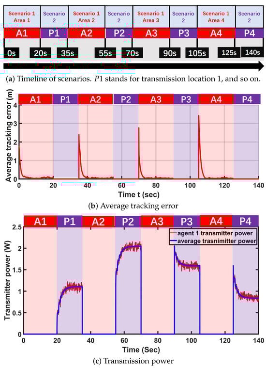
Figure 7. (a) Time evolution of scenarios. This reveals the process of the sensing networks’ workflow with respect to time. (b) Time evolution of the normalized tracking error on the x axis (red curve) and y axis (blue curve). (c) Time evolution of the transmission power for a single agent (red curve) and the population average (blue curve).

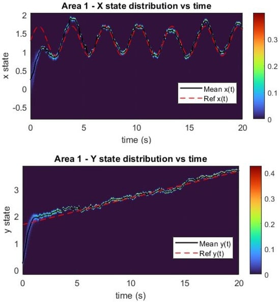
Figure 8. Navigation state density distribution evolution.

To further analyze the learning performance at the individual agent level, I examine the HJB equation residual of Robot 1 in Scenario 1 (i.e., navigation). Figure 9 plots the HJB residual over time in a stationary setting, where both the HJB and FPK equations are assumed to be time-invariant. In this scenario, the mass neural network is updated every 1 s to compute $\mathbb{E}\left[m_s\left(e_s\right)\right]$, which is then used to update the critic neural network. As shown in Figure 9, the HJB residual converges to zero within approximately 1 s. Moreover, the HJB error distribution among all robots is plotted in Figure 10.

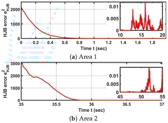
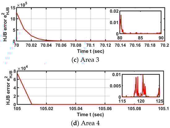
Figure 9. The plots of Robot 1’s HJB equation error, which is also the critic NN error. The small figure on the right part of each plot is the HJB error in the last 10 s of moving in each area.

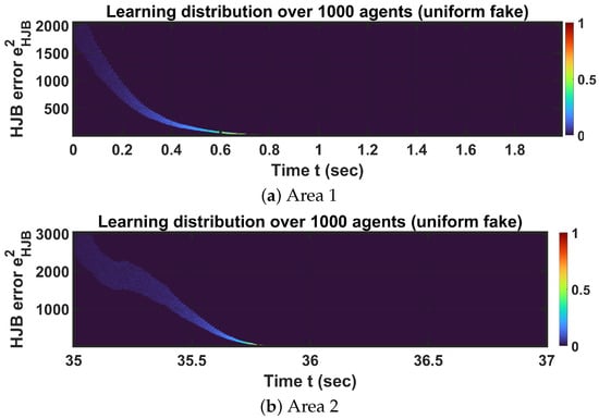
Figure 10. The plots of all robots’ HJB error distributions.

Given the convergence of both the tracking error and the HJB residual, it can be concluded that the actor, critic, and mass networks successfully converge in Scenario 1. This implies that the learned control policy, value function, and tracking error distribution converge to the solution of the mean field equation system. Therefore, the learned control policy represents the unique solution to the ${ϵ}_N$-Nash equilibrium.

Next, I analyze the performance of the Actor–Critic–Mass (ACM) algorithm in Scenario 2 (i.e., transmission). Similarly to Scenario 1, a set of three neural networks is employed to solve the coupled HJB–FPK equation system for decentralized optimal transmission power control. The evolution of the signal-to-interference-plus-noise ratio (SINR) during data transmission is shown in Figure 11. Furthermore, the SINR distribution is also plotted in Figure 12. As observed, the SINR converges to the desired target of $0.6$, confirming the effectiveness of the ACM algorithm in transmission tasks.

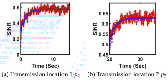
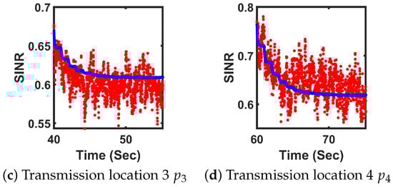
Figure 11. The plots of the average SINR and Robot 1’s SINR in all transmission locations. The red dots show Robot 1’s SINR and the blue dots represent the average SINR among all robots.

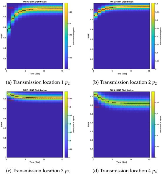
Figure 12. SINR distribution plot.

Interestingly, at transmission locations $p_3$ and $p_4$, the initial SINR values are higher but subsequently decrease and stabilize near the target value. This behavior arises from the value function design in Equation (14), which penalizes high power outputs due to the energy constraints of the low-cost mobile sensing robots. Figure 7c further illustrates that during data transmission at $p_3$ and $p_4$, the robot actively minimizes its SINR to reduce power consumption at the transmitter.

This power-saving behavior will next be compared with the performance of an alternative decentralized game theoretic method, namely the Parallel Update Algorithm (PUA) introduced in [41].

7. Results and Analysis

To evaluate the effectiveness of the proposed ACM algorithm, it is compared with the Parallel Update Algorithm (PUA) introduced in [41]. The parameters for the PUA algorithm are selected as $L=u=1$, ${\sigma }^2=0.1$, and $\lambda =0.78$, ensuring that the target SINR $\mu =0.6$ is achieved.

The transmission process in area $A_1$ is simulated using both the proposed ACM algorithm and the PUA algorithm. As shown in Figure 13, both methods achieve the target SINR. Furthermore, the total transmission power consumption across all agents converges to the same level, confirming that both algorithms reach a Nash equilibrium, as established in [41]. This validates the capability of the ACM algorithm to learn the optimal decentralized transmission strategy.

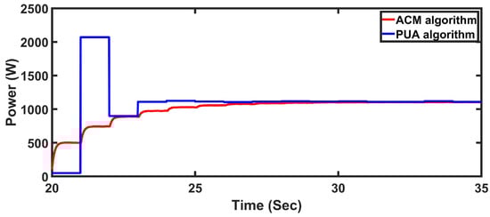
Figure 13. The transmitters’ power summation for all mobile sensing robots in Scenario 2. The red curve represents the ACM algorithm. The blue curve represents the PUA algorithm.

However, it is important to highlight key differences. The ACM algorithm updates neural network weights continuously, while the PUA algorithm performs updates every 1 s. The ACM algorithm uses $8.59\%$ less power than the PUA algorithm. Despite its slower update frequency, PUA converges faster to the Nash equilibrium. This is because the PUA algorithm does not explicitly account for the population influence (i.e., the mass effect), leading to a more aggressive strategy.

Nevertheless, Figure 13 clearly shows that the PUA algorithm results in higher transmission power levels compared to the ACM algorithm, particularly during the transmission intervals at $p_3$ and $p_4$. Such power profiles are not ideal for energy-constrained mobile sensors. In contrast, the ACM algorithm, by modeling and responding to the mean field, promotes more energy-efficient behavior.

To evaluate the overall performance, a composite cost function that penalizes both SINR deviation and power consumption is defined:

$$\begin{array}{c}\hfill J\left(t\right)={\displaystyle \frac{1}{N}}{\int }_t^T\left[\sum _{i=1}^N\left({\widehat{\mu }}_i\left(\tau \right)-\mu \right)+\sum _{i=1}^N{p}_i\left(\tau \right)\right]d\tau .\end{array}$$

(48)

The values of $J\left(t\right)$ for both algorithms are plotted in Figure 14. The results demonstrate that the ACM algorithm achieves superior performance by maintaining SINR requirements while minimizing power consumption.

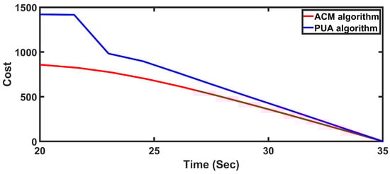
Figure 14. The transmitters’ cost for all sensing robots in Scenario 2. The red curve represents the ACM algorithm. The blue curve represents the PUA algorithm.

Notably, at approximately 21 s in Figure 13, the PUA algorithm exhibits an overshoot in total power. This behavior stems from its lack of coordination and foresight—each agent increases its transmission power independently, without considering the collective dynamics. In contrast, the ACM algorithm anticipates these interactions by estimating the power distribution (via the mass NN), thereby avoiding destructive competition.

This comparison highlights a fundamental advantage of Mean Field Games: they serve as an implicit coordination mechanism in non-cooperative multi-agent systems. Through mass feedback, each agent adapts to the aggregate behavior of the population without requiring explicit communication, enabling convergence to a socially efficient $ϵ$-Nash equilibrium. Moreover, this feature significantly reduces communication overheads and channel usage, making ACM particularly well-suited for large-scale mobile sensor networks.

8. Discussion

The proposed Actor–Critic–Mass (ACM) algorithm demonstrates scalable, decentralized optimization for large-scale mobile wireless sensor networks (MWSNs). By jointly solving the Hamilton–Jacobi–Bellman (HJB) and Fokker–Planck–Kolmogorov (FPK) equations through reinforcement learning, the ACM enables each agent to learn optimal control policies without inter-agent communication. The simulation results confirm that ACM maintains the desired signal-to-interference-plus-noise ratio (SINR) while minimizing transmission power, offering energy-efficient performance under dynamic network conditions.

Compared with recent reinforcement learning approaches, ACM provides comparable or superior energy savings while avoiding centralized coordination. El Jamous et al. [42] achieved energy-efficient WiFi power control using deep RL but relied on a global critic and full state feedback. Choi et al. [43] reported up to 70% power savings in 5G H-CRANs through centralized interference coordination, whereas ACM attains similar gains using only local feedback and the learned mean field distribution. Likewise, Soltani et al. [44] demonstrated efficiency improvements in MARL-based routing but required synchronized updates, in contrast to ACM’s asynchronous and fully distributed updates.

The observed convergence of the HJB residuals and SINR trajectories aligns with mean field control theory, which predicts ${ϵ}_N$-Nash convergence as $N\to \infty$ [15]. Unlike earlier mean field control formulations that depend on offline PDE solutions [45], ACM learns the evolving population density online, achieving faster adaptation under stochastic conditions. This emergent, energy-aware coordination behavior is comparable to that seen in other MFG-based cooperative systems such as autonomous driving [46].

9. Conclusions

This paper presents a novel decentralized co-optimization framework for mobile sensing and communication in large-scale wireless sensor networks, based on Mean Field Game (MFG) theory. The proposed Actor–Critic–Mass (ACM) algorithm leverages three neural networks—Actor NN, Critic NN, and Mass NN—to approximate the solution of the coupled Hamilton–Jacobi–Bellman (HJB) and Fokker–Planck–Kolmogorov (FPK) equations online. Two value functions are formulated to capture both navigation and communication objectives. Minimizing these functions ensures that the desired SINR is maintained and that the sensing agents accurately follow designated trajectories. The ACM algorithm achieved $2.32\%$ trajectory tracking accuracy and uses $8.59\%$ less power than the PUA algorithm. The resulting optimal policies are shown to approximate an $ϵ$-Nash equilibrium. Compared with traditional centralized and distributed optimization algorithms, the ACM framework significantly reduces communication overhead and computational complexity, enabling scalable, real-time implementation. Numerical simulations validate the effectiveness and efficiency of the approach, demonstrating high tracking accuracy and energy-efficient transmission.

Limitations: Despite these promising results, several simplifying assumptions constrain the present study. First, all agents were assumed to be homogeneous with identical dynamics and sensing capabilities; extending the framework to heterogeneous agents with distinct models and cost functions remains an open challenge. Second, communication latency, packet loss, and synchronization issues were neglected, yet such factors can significantly influence decentralized learning and coordination performance in practice. Third, the convergence guarantees rely on the infinite-population (mean field) limit, while practical deployments involve finite populations whose deviations from the mean field warrant further theoretical characterization. Future work will relax these assumptions by incorporating asynchronous updates, heterogeneous agent dynamics, and realistic wireless channel models to more accurately capture large-scale multi-agent behaviors in real-world environments.

Future Perspectives: Building on these results, several promising directions remain open. First, extending the ACM framework to heterogeneous multi-agent systems, where agents differ in sensing and communication capabilities, would improve applicability to realistic networks. Second, incorporating safety constraints, robustness against adversarial disturbances, and energy awareness into the MFG formulation is essential for deployment in safety-critical domains. Third, coupling ACM with online system identification or adaptive learning strategies could enhance robustness to dynamic or partially observed environments. Finally, exploring hierarchical and multi-layered networked systems—such as UAV–AUV–ground cooperative networks—offers a path toward general-purpose autonomous sensing and communication in real-world applications.

In practical deployments, additional challenges such as sensor drifts, intermittent communication, and packet loss can significantly affect system performance. Small but accumulating sensor drifts may distort the agents’ state estimates and consequently the learned mean field distribution. Future work will therefore incorporate online calibration mechanisms and adaptive filtering to mitigate such errors. Similarly, communication failures or delays can cause asynchronous updates among agents, leading to instability in distributed learning. To address this, we plan to integrate resilient consensus and delay compensation strategies into the ACM framework, allowing agents to maintain stability even under partial or delayed information exchange. These efforts will be validated through experiments on the planned large-scale mobile sensing testbed to ensure robustness under realistic operating conditions.

References

- Liu, L.; Zheng, Z.; Zhu, S.; Chan, S.; Wu, C. Virtual-Mobile-Agent-Assisted Boundary Tracking for Continuous Objects in Underwater Acoustic Sensor Networks. IEEE Internet Things J. 2024, 11, 9171–9183. [Google Scholar] [CrossRef]
- Huang, P.; Zeng, L.; Chen, X.; Luo, K.; Zhou, Z.; Yu, S. Edge Robotics: Edge-Computing-Accelerated Multirobot Simultaneous Localization and Mapping. IEEE Internet Things J. 2022, 9, 14087–14102. [Google Scholar] [CrossRef]
- Fernández-Jiménez, F.J.; Dios, J.R.M.d. A Robot–Sensor Network Security Architecture for Monitoring Applications. IEEE Internet Things J. 2022, 9, 6288–6304. [Google Scholar] [CrossRef]
- Lee, J.S.; Jiang, H.T. An Extended Hierarchical Clustering Approach to Energy-Harvesting Mobile Wireless Sensor Networks. IEEE Internet Things J. 2021, 8, 7105–7114. [Google Scholar] [CrossRef]
- Su, Y.; Guo, L.; Jin, Z.; Fu, X. A Mobile-Beacon-Based Iterative Localization Mechanism in Large-Scale Underwater Acoustic Sensor Networks. IEEE Internet Things J. 2021, 8, 3653–3664. [Google Scholar] [CrossRef]
- Wang, D.; Chen, H.; Lao, S.; Drew, S. Efficient Path Planning and Dynamic Obstacle Avoidance in Edge for Safe Navigation of USV. IEEE Internet Things J. 2024, 11, 10084–10094. [Google Scholar] [CrossRef]
- Ma, C.; Li, A.; Du, Y.; Dong, H.; Yang, Y. Efficient and scalable reinforcement learning for large-scale network control. Nat. Mach. Intell. 2024, 6, 1006–1020. [Google Scholar] [CrossRef]
- Huang, M.; Caines, P.E.; Charalambous, C.D. Stochastic power control for wireless systems: Classical and viscosity solutions. In Proceedings of the 40th IEEE Conference on Decision and Control (Cat. No. 01CH37228), Orlando, FL, USA, 4–7 December 2001; Volume 2, pp. 1037–1042. [Google Scholar]
- Kafetzis, D.; Vassilaras, S.; Vardoulias, G.; Koutsopoulos, I. Software-defined networking meets software-defined radio in mobile ad hoc networks: State of the art and future directions. IEEE Access 2022, 10, 9989–10014. [Google Scholar] [CrossRef]
- Zejian, Z.; Xu, H. Decentralized Adaptive Optimal Tracking Control for Massive Multi-agent Systems: An Actor-Critic-Mass Algorithm. In Proceedings of the 58th IEEE Conference on Decision and Control, Nice, France, 11–13 December 2019. [Google Scholar]
- Zejian, Z.; Xu, H. Decentralized Adaptive Optimal Control for Massive Multi-agent Systems Using Mean Field Game with Self-Organizing Neural Networks. In Proceedings of the 58th IEEE Conference on Decision and Control, Nice, France, 11–13 December 2019. [Google Scholar]
- Guéant, O.; Lasry, J.M.; Lions, P.L. Mean field games and applications. In Paris-Princeton Lectures on Mathematical Finance 2010; Springer: Berlin/Heidelberg, Germany, 2011; pp. 205–266. [Google Scholar]
- Lasry, J.M.; Lions, P.L. Mean field games. Jpn. J. Math. 2007, 2, 229–260. [Google Scholar] [CrossRef]
- Prag, K.; Woolway, M.; Celik, T. Toward data-driven optimal control: A systematic review of the landscape. IEEE Access 2022, 10, 32190–32212. [Google Scholar] [CrossRef]
- Huang, M.; Caines, P.E.; Malhamé, R.P. Large-population cost-coupled LQG problems with nonuniform agents: Individual-mass behavior and decentralized ε-Nash equilibria. IEEE Trans. Autom. Control 2007, 52, 1560–1571. [Google Scholar] [CrossRef]
- Huang, M.; Sheu, S.; Sun, L. Mean field social optimization: Feedback person-by-person optimality and the dynamic programming equation. In Proceedings of the 2020 59th IEEE Conference on Decision and Control (CDC), Jeju, Republic of Korea, 14–18 December 2020. [Google Scholar]
- Cardaliaguet, P.; Porretta, A. An Introduction to Mean Field Game Theory; Springer: Berlin/Heidelberg, Germany, 2021; pp. 1–158. [Google Scholar]
- Liu, M.; Zhao, L.; Lopez, V.; Wan, Y.; Lewis, F.; Tseng, H.E.; Filev, D. Game-Theoretic Decision-Making for Autonomous Driving; CRC Press: Boca Raton, FL, USA, 2025; pp. 236–272. [Google Scholar]
- Wei, X.; Zhao, J.; Zhou, L.; Qian, Y. Broad Reinforcement Learning for Supporting Fast Autonomous IoT. IEEE Internet Things J. 2020, 7, 7010–7020. [Google Scholar] [CrossRef]
- Liang, S.; Wang, X.; Huang, J. Actor–Critic Reinforcement Learning Algorithms for Mean Field Games in Continuous Time, State, and Action Spaces. arXiv 2024, arXiv:2401.00052. [Google Scholar] [CrossRef]
- Angiuli, A.; Subramanian, J.; Perolat, J.; Carpentier, A.; Geist, M.; Pietquin, O. Deep Reinforcement Learning for Mean Field Control and Games. arXiv 2023, arXiv:2309.10953. [Google Scholar]
- Bogunovic, I.; Pirotta, M.; Rosolia, U. Safe-M3-UCRL: Safe Mean-Field Multi-Agent Reinforcement Learning under Global Constraints. In Proceedings of the 23rd International Conference on Autonomous Agents and Multiagent Systems (AAMAS), Auckland, New Zealand, 6–10 May 2024; pp. 973–981. [Google Scholar]
- Zaman, A.; Ratliff, L.; Mesbahi, M. Robust Multi-Agent Reinforcement Learning via Mean-Field Games. In Proceedings of the 41st International Conference on Machine Learning (ICML), Vienna, Austria, 21–27 July 2024. [Google Scholar]
- Jiang, Y.; Xu, K.; Wu, Y.; Zhang, M. A Survey of Fully Decentralized Multi-Agent Reinforcement Learning. arXiv 2024, arXiv:2306.02766. [Google Scholar]
- Gabler, L.; Scheller, S.; Albrecht, S.V. Decentralized Actor–Critic Reinforcement Learning for Cooperative Tasks with Sparse Rewards. Front. Robot. AI 2024, 11, 1229026. [Google Scholar]
- Gu, Y. Centralized training with hybrid execution in multi-agent reinforcement learning via predictive observation imputation. Artif. Intell. 2025, 348, 104404. [Google Scholar] [CrossRef]
- Alam, S.; Khan, M.; Zhang, W. Actor–Critic Frameworks for UAV Swarm Networks: A Survey. Drones 2025, 9, 153. [Google Scholar] [CrossRef]
- Xu, C.; Li, P.; Sun, X. Mean-Field Multi-Agent Reinforcement Learning for UAV-Assisted V2X Communications. arXiv 2025, arXiv:2502.01234. [Google Scholar]
- Emami, N.; Joo, C.; Kim, S.C. Age of Information Minimization Using Multi-Agent UAVs Based on AI-Enhanced Mean Field Resource Allocation. IEEE Trans. Wirel. Commun. 2024, 73, 13368–13380. [Google Scholar] [CrossRef]
- Mostofi, Y.; Malmirchegini, M.; Ghaffarkhah, A. Estimation of communication signal strength in robotic networks. In Proceedings of the 2010 IEEE International Conference on Robotics and Automation, Anchorage, AK, USA, 3–7 May 2010; pp. 1946–1951. [Google Scholar]
- Malmirchegini, M.; Mostofi, Y. On the spatial predictability of communication channels. IEEE Trans. Wirel. Commun. 2012, 11, 964–978. [Google Scholar] [CrossRef]
- Charalambous, C.D.; Menemenlis, N. Stochastic models for long-term multipath fading channels and their statistical properties. In Proceedings of the 38th IEEE Conference on Decision and Control (Cat. No. 99CH36304), Phoenix, AZ, USA, 7–10 December 1999; Volume 5, pp. 4947–4952. [Google Scholar]
- Huang, M.; Malhamé, R.P.; Caines, P.E. Stochastic power control in wireless communication systems: Analysis, approximate control algorithms and state aggregation. In Proceedings of the 42nd IEEE International Conference on Decision and Control (IEEE Cat. No. 03CH37475), Maui, HI, USA, 9–12 December 2003; Volume 4, pp. 4231–4236. [Google Scholar]
- Huang, M.; Caines, P.E.; Malhamé, R.P. Individual and mass behaviour in large population stochastic wireless power control problems: Centralized and Nash equilibrium solutions. In Proceedings of the 42nd IEEE International Conference on Decision and Control (IEEE Cat. No. 03CH37475)), Maui, HI, USA, 9–12 December 2003; Volume 1, pp. 98–103. [Google Scholar]
- Aziz, M.; Caines, P.E. Computational investigations of decentralized cellular network optimization via mean field control. In Proceedings of the 53rd IEEE Conference on Decision and Control, Los Angeles, CA, USA, 15–17 December 2014; pp. 5560–5567. [Google Scholar]
- Aziz, M.; Caines, P.E. A mean field game computational methodology for decentralized cellular network optimization. IEEE Trans. Control Syst. Technol. 2016, 25, 563–576. [Google Scholar] [CrossRef]
- Haenggi, M.; Ganti, R.K. Interference in large wireless networks. Found. Trends Netw. 2009, 3, 127–248. [Google Scholar] [CrossRef]
- Baccelli, F.; Błaszczyszyn, B. Stochastic geometry and wireless networks: Volume II applications. Found. Trends Netw. 2010, 4, 1–312. [Google Scholar] [CrossRef]
- Jiang, Y.; Fan, J.; Chai, T.; Lewis, F.L.; Li, J. Tracking control for linear discrete-time networked control systems with unknown dynamics and dropout. IEEE Trans. Neural Netw. Learn. Syst. 2017, 29, 4607–4620. [Google Scholar] [CrossRef] [PubMed]
- Nourian, M.; Caines, P.E. ϵ-Nash mean field game theory for nonlinear stochastic dynamical systems with major and minor agents. SIAM J. Control Optim. 2013, 51, 3302–3331. [Google Scholar] [CrossRef]
- Alpcan, T.; Başar, T.; Srikant, R.; Altman, E. CDMA uplink power control as a noncooperative game. Wirel. Netw. 2002, 8, 659–670. [Google Scholar] [CrossRef]
- El Jamous, Z.; Davaslioglu, K.; Sagduyu, Y.E. Deep reinforcement learning for power control in next-generation wifi network systems. In Proceedings of the MILCOM 2022—2022 IEEE Military Communications Conference (MILCOM), Rockville, MD, USA, 28 November–2 December 2022; pp. 547–552. [Google Scholar]
- Choi, H.; Kim, T.; Lee, S.; Choi, H.S.; Yoo, N. Energy-Efficient Dynamic Enhanced Inter-Cell Interference Coordination Scheme Based on Deep Reinforcement Learning in H-CRAN. Sensors 2024, 24, 7980. [Google Scholar] [CrossRef]
- Soltani, P.; Eskandarpour, M.; Ahmadizad, A.; Soleimani, H. Energy-Efficient Routing Algorithm for Wireless Sensor Networks: A Multi-Agent Reinforcement Learning Approach. arXiv 2025, arXiv:2508.14679. [Google Scholar]
- Wu, Y.; Wu, J.; Huang, M.; Shi, L. Mean-field transmission power control in dense networks. IEEE Trans. Control Netw. Syst. 2020, 8, 99–110. [Google Scholar] [CrossRef]
- Zhang, H.; Lu, C.; Tang, H.; Wei, X.; Liang, L.; Cheng, L.; Ding, W.; Han, Z. Mean-field-aided multiagent reinforcement learning for resource allocation in vehicular networks. IEEE Internet Things J. 2022, 10, 2667–2679. [Google Scholar] [CrossRef]
- Zhou, Z.; Qian, L.; Xu, H. Decentralized multi-agent reinforcement learning for large-scale mobile wireless sensor network control using mean field games. In Proceedings of the 2024 33rd International Conference on Computer Communications and Networks (ICCCN), Kailua-Kona, HI, USA, 29–31 July 2024; pp. 1–6. [Google Scholar]
Disclaimer/Publisher’s Note: The statements, opinions and data contained in all publications are solely those of the individual author(s) and contributor(s) and not of MDPI and/or the editor(s). MDPI and/or the editor(s) disclaim responsibility for any injury to people or property resulting from any ideas, methods, instructions or products referred to in the content. |
© 2025 by the author. Licensee MDPI, Basel, Switzerland. This article is an open access article distributed under the terms and conditions of the Creative Commons Attribution (CC BY) license (https://creativecommons.org/licenses/by/4.0/).