Design and Real-Time Application of Explicit Model-Following Techniques for Nonlinear Systems in Reciprocal State Space

Abstract

This paper presents an efficient algorithm for Explicit Model-Following (EMF) control using an Output-derivative Feedback Control (OFC) scheme within the Reciprocal State Space (RSS) framework, aimed at overcoming the performance limitations associated with state-derivative dependence. For Lipschitz Nonlinear Systems (LNS), two approaches are proposed: a linear EMF (LEMF) strategy, which transforms the system into a Linear Parameter-Varying (LPV) representation via the Differential Mean Value Theorem (DMVT) to facilitate controller design, and a nonlinear EMF (NEMF) scheme, which enables the direct tracking of a nonlinear reference model. The stability of the closed-loop system is ensured by deriving control gains through Linear Quadratic Regulator (LQR) optimization. The proposed algorithms are validated through Real-Time Implementation (RTI) on an Arduino DUE platform, demonstrating their effectiveness and practical feasibility.

1. Introduction

Historically, expressing a system in the Standard State Space (SSS) form or in the transfer function form and using state or output feedback comprised a widely adopted approach for developing efficient and reliable control algorithms [1,2,3]. This methodology is particularly valued for its flexibility in handling various system representations [4,5,6,7,8]. Nevertheless, it faces inherent challenges, especially in real-time applications where some systems cannot be modeled in SSS form or when state-related signals are not easily accessible for feedback design. For instance, systems that exhibit open-loop behavior at infinity—such as singular systems—cannot be represented in SSS form, which renders conventional control and regulation methods ineffective. Furthermore, in many practical processes, sensors often measure state-derived quantities rather than the state variables themselves. In such cases, it is more appropriate to use feedback derived from state derivatives rather than from the states directly. This approach can help avoid the need for integrators, which may add complexity and cost to the control system implementation [9,10].

Such systems, involving output and/or state derivatives, are frequently encountered in various domains, including electrical, aerospace, and chemical systems [11,12,13]. In this context, several studies have proposed different control law synthesis approaches that address stabilization, sliding-mode control, and tracking problems via state- or output-derivative feedback in the RSS framework. These methods have been developed for both linear [14,15] and nonlinear systems [16,17]. Moreover, state-derivative feedback in RSS form has facilitated the implementation of well-established control methodologies such as pole placement, eigen-structure assignment, and LQR optimization [18,19].

Model-following approaches, as a subset of LQR-based techniques, aim to align a system’s performance output with a desired reference model. Although the closed-loop system may not perfectly replicate the model’s behavior, asymptotic stability is guaranteed. Such designs are attractive for their simplicity and cost-effectiveness, as they typically require fewer sensors and actuators compared to the number of system states—an advantage particularly relevant in large-scale or structural control applications.

Motivated by the limitations of existing methods [16,20] and the need for improved real-time implementability, this paper proposes a novel EMF approach for LNS within the RSS framework. Building upon the foundational work in [16], the proposed method integrates derivative output feedback with LQR-based gain synthesis and applies the DMVT to handle nonlinearities. The main contributions of this study are summarized as follows:

• An EMF design was developed based on derivative output feedback in the RSS framework, in contrast to conventional SSS-based approaches.
• The derivative Lipschitz property was integrated into the OFC design, where the nonlinear system is converted into an LPV representation via the principles of the DMVT.
• The reference model was explicitly included in the controller as a feed-forward compensator that drives the plant states to zero, ensuring the performance output closely tracks the model output.
• Previous RSS-based model-following designs were extended, such as [21], to nonlinear systems through the combined use of the DMVT and LQR-based optimization, enabling the explicit treatment of nonlinearities while maintaining analytical tractability and stability guarantees. The proposed design was experimentally validated through real-time HIL implementation on an Arduino DUE platform, confirming its practical feasibility.
• In contrast to recent nonlinear control strategies—such as cooperative adaptive fuzzy control for large-scale cyber-physical systems, resilient decentralized control under DoS attacks, and neural-network-based fault-tolerant schemes—the proposed EMF approach provides an explicit, optimization-based framework that remains computationally lightweight and well suited for embedded real-time applications, avoiding complex approximators while preserving transparency in controller synthesis.

The remainder of this paper is organized as follows: Section 2 presents the problem formulation and preliminaries. Section 3 details the LEMF feedback control design, which incorporates derivative output variables and employs the principles of the DMVT for LNS in RSS form. Section 4 discusses the extension to the NEMF method based on the derivative Lipschitz property. Section 5 provides the RTI results, demonstrating the effectiveness of the proposed approach on an Arduino DUE-based HIL platform.

• Notation: The notation outlined below will be used throughout this paper:

• $tr\left(\overline{V}\right)$ is the trace of matrix $\overline{V}$; ${\overline{V}}^T$ is the transposed matrix of $\overline{V}$;
• For a square matrix $\overline{V}$, the notation $\overline{V}>0$ ($\overline{V}<0$) means that $\overline{V}$ is positive definite (negative definite);
• The set $Co(\overline{a},\overline{b})=\{\alpha \overline{a}+(1-\alpha )\overline{b},0\le \alpha \le 1\}$ is the convex hull of $\overline{a},\overline{b}$;
• $l_n\left(j\right)={\left(\begin{array}{c}\underbrace{0,\dots ,0,\stackrel{j^{th}}{\overbrace{1}},0,\dots ,0}\\ n-components\end{array}\right)}^T\in {\mathbb{R}}^n$, $n\ge 1$, is the vector of the canonical basis of ${\mathbb{R}}^n$.

2. Preliminary and Problem Position

The concept of the RSS is introduced as a specific case of linear singular systems. Two approaches for linear and nonlinear systems have been explored in [16,18]. In this context, two main approaches to modeling the new RSS framework have been considered: one approach involves converting the nonlinear singular system, while the other directly incorporates state derivatives in the system representation. Additionally, the mathematical properties of the controllability, stability, and uniqueness of the solution have been thoroughly examined in [11,13,16]. Consider now the following nonlinear dynamic system expressed in RSS form:

$$\left\{\begin{array}{c}\overline{x}\left(t\right)=\overline{A}\overline{\dot{x}}\left(t\right)+\overline{B}\overline{u}\left(t\right)+\overline{\mathit{\varphi }}(\overline{\dot{x}}\left(t\right),t)\hfill \\ \overline{y}\left(t\right)=\overline{C}\overline{\dot{x}}\left(t\right)\hfill \end{array}\right.$$

(1)

where $\overline{x}\left(t\right)\in {\mathbb{R}}^n$, $\overline{u}\left(t\right)\in {\mathbb{R}}^m$, and $\overline{y}\left(t\right)\in {\mathbb{R}}^p$ are, respectively, the state vector, the input vector, and the output vector. $\overline{\mathit{\varphi }}:{\mathbb{R}}^n\to {\mathbb{R}}^q$ is a Lipschitz-continuous nonlinear vector function. Matrices $\overline{A}$, $\overline{B}$, and $\overline{C}$ are constant and have appropriate dimensions. Then the following lemmas are addressed in this brief:

Lemma 1

([22]). Let us consider the following nonlinear function: $\underline{\chi }:{\mathbb{R}}^n\to {\mathbb{R}}^n$. The following two elements are equivalent:

• χ is globally Lipschitz with respect to its argument, i.e.,

  $$\Vert \chi \left(\overline{a}\right)-\chi \left(\overline{b}\right)\Vert ⩽{\theta }_{\chi }\Vert \overline{a}-\overline{b}\Vert ,\forall \overline{a},\overline{b}\in {\mathbb{R}}^n.$$

  (2)
• There are constants $\underline{{\chi }_{ij}}$ and $\overline{{\chi }_{ij}}$ so that for all $\forall \overline{a},\overline{b}\in$${\mathbb{R}}^n$, there exist $n_i\in Co(\overline{a},\overline{b})$, $n_i\ne \overline{a}$, $n_i\ne \overline{b}$ and functions ${\chi }_{ij}:{\mathbb{R}}^n\times {\mathbb{R}}^n⟶\mathbb{R}$ satisfying the following equality:

  $$\chi \left(\overline{a}\right)-\chi \left(\overline{b}\right)={\displaystyle \sum _{i,j=1}^{q,n}}{\chi }_{ij}\left(n_i\right){∆}_{ij}(\overline{a}-\overline{b})$$

  (3)

  and $\underline{{\chi }_{ij}}⩽{\chi }_{ij}\left(z_i\right)⩽\overline{{\chi }_{ij}}$ where ${\chi }_{ij}\left(n_i\right)={\displaystyle \frac{\partial {\chi }_i}{\partial {\overline{a}}_j}}\left(n_i\right)$ and ${∆}_{ij}=l_q\left(i\right)l_n^T\left(j\right)$.

Lemma 2

([23]). Let $\overline{M}$ and $\overline{N}$ be two matrices of appropriate dimensions. Then, the following inequality is valid for any constant $\overline{\eta }>0$:

$${\overline{M}}^T\overline{N}+{\overline{N}}^T\overline{M}\le \overline{\eta }{\overline{M}}^T\overline{M}+{\overline{\eta }}^{-1}{\overline{N}}^T\overline{N}$$

(4)

Remark on impulsive modes:

The present analysis is restricted to regular and causal LNS, which inherently exclude impulsive dynamics.

It is important to note that the Reciprocal State Space (RSS) framework can be interpreted as a particular case of singular systems. However, in the present study, we restrict the analysis to LNSs that satisfy the regularity and causality conditions, which exclude impulsive solutions. The exclusion of impulsive modes implies that the proposed design applies to regular, causal singular systems without impulsive behavior. Consequently, descriptor systems exhibiting impulsive dynamics or an index higher than one are not directly covered by this study, although the extension to such systems is a promising direction for future work. It is worth noting that extending the proposed EMF methodology to descriptor systems with impulsive or high-index behavior would require additional developments in solvability analysis and index reduction. Such an extension would involve reformulating the stability proof using differential–algebraic frameworks and regularization techniques. Although this topic lies beyond the present scope, it represents a promising direction for future investigations.

This brief aims to create an EMF design with derivative OFC for LNS within the RSS framework, ensuring that the performance output closely follows the model’s output and guaranteeing the asymptotic stability of the closed-loop system through the application of LQR techniques.

3. Explicit Model-Following Design

In this section, two approaches are developed according to the choice of EMF in the performance output case for LNS in RSS form.

3.1. Linear EMF

The objective is to determine a straightforward derivative OFC law of the following form:

$$\overline{u}\left(t\right)=-\overline{{\Gamma }_y}\overline{y}\left(t\right)$$

(5)

where $\overline{{\Gamma }_y}\in {\mathbb{R}}^{m\times n}$. Next, by substituting (5) into (1), the closed-loop system is obtained as follows:

$$\overline{x}\left(t\right)=(\overline{A}-\overline{B}\overline{{\Gamma }_y}\overline{C})\overline{\dot{x}}\left(t\right)+\overline{\mathit{\varphi }}(\overline{\dot{x}}\left(t\right),t)$$

(6)

Assume that the performance output ${\overline{\mathrm{Y}}}_F$, composed of state derivatives, is given by the following:

$${\overline{\mathrm{Y}}}_F={\overline{M}}_F\overline{\dot{x}}\left(t\right)$$

(7)

The key output information is represented by the performance output ${\overline{\mathrm{Y}}}_F$, which may not be directly measurable within the system. The desired linear model that the controlled system aims to follow is given by the following:

$$\left\{\begin{array}{c}{\overline{x}}_M\left(t\right)={\overline{A}}_M{\overline{\dot{x}}}_M\left(t\right)\\ {\overline{y}}_M\left(t\right)={\overline{C}}_M{\overline{\dot{x}}}_M\left(t\right);{\overline{\mathrm{Y}}}_M={\overline{M}}_M{\overline{\dot{x}}}_M\left(t\right)\end{array}\right.$$

(8)

To ensure that (1) is asymptotically stable and adheres to the model (8), the following derivative OFC law is proposed:

Theorem 1.

For LNS (1) with OFC (5), the RSS closed-loop system is asymptotically stable if there exists a matrix $\overline{U}$ of appropriate dimensions and SPD matrices $\overline{P}$, $\overline{D}$, and $\overline{R}$, such that the following coupled equations are solvable:

$$\left\{\begin{array}{c}{\overline{\Lambda }}_1=block-diag({\overline{\Xi }}_1\left({\zeta }^1\right),\dots ,{\overline{\Xi }}_1\left({\zeta }^{2^{nq}}\right))=0\hfill \\ {\overline{\Lambda }}_2=block-diag({\overline{\Xi }}_2\left({\zeta }^1\right),\dots ,{\overline{\Xi }}_2\left({\zeta }^{2^{nq}}\right))=0\hfill \\ {\overline{\Lambda }}_3=block-diag({\overline{\Xi }}_3\left({\zeta }^1\right),\dots ,{\overline{\Xi }}_3\left({\zeta }^{2^{nq}}\right))=0\hfill \end{array}\right.$$

(9)

where ${\zeta }^i\in {\mathcal{H}}_{{\mathcal{M}}_{nq}}$ and

$$\left\{\begin{array}{c}{\overline{\Xi }}_1={\displaystyle \frac{\partial \tilde{\Lambda }}{\partial \overline{U}}}=\overline{P}{\mathcal{A}}_c+{\mathcal{A}}_c^T\overline{P}+\overline{D}+{\mathcal{C}}^T{\overline{\Gamma }}_y^T\overline{R}{\overline{\Gamma }}_y\mathcal{C}=0\hfill \\ {\overline{\Xi }}_2={\displaystyle \frac{\partial \tilde{\Lambda }}{\partial \overline{P}}}={\mathcal{A}}_c\overline{U}+\overline{U}{\mathcal{A}}_c^T+\overline{O}=0\hfill \\ {\overline{\Xi }}_3={\displaystyle \frac{\partial \tilde{\Lambda }}{\partial {\underline{\Gamma }}_y}}=\overline{R}{\underline{\Gamma }}_y\mathcal{C}\overline{U}{\mathcal{C}}^T-{\mathcal{B}}^T\overline{P}\overline{U}{\mathcal{C}}^T=0\hfill \end{array}\right.$$

(10)

with

$${\underline{\Gamma }}_y={\overline{R}}^{-1}{\mathcal{B}}^T\overline{P}\overline{U}{\mathcal{C}}^T{\left(\mathcal{C}\overline{U}{\mathcal{C}}^T\right)}^{-1}$$

(11)

Proof. 

First, the model error $\epsilon$ is defined as follows:

$$\epsilon ={\overline{{\rm Y}}}_M-{\overline{{\rm Y}}}_F={\overline{M}}_M{\overline{\dot{x}}}_M\left(t\right)-{\overline{M}}_F\overline{\dot{x}}\left(t\right)$$

(12)

where the sizes of matrices ${\overline{\mathrm{Y}}}_M$ and ${\overline{\mathrm{Y}}}_F$ must be the same. Next, by considering the augmented state as $x={\left[\begin{array}{cc}\overline{x}& {\overline{x}}_M\end{array}\right]}^T$, the augmented system will be expressed as follows:

$$x\left(t\right)=\underset{A}{\underbrace{\left[\begin{array}{cc}\overline{A}& 0\\ 0& {\overline{A}}_M\end{array}\right]}}\dot{x}\left(t\right)+\underset{B}{\underbrace{\left[\begin{array}{c}\overline{B}\\ 0\end{array}\right]}}u\left(t\right)+\underset{\overline{\Phi }(\dot{x}\left(t\right),t)}{\underbrace{\left[\begin{array}{c}I\\ 0\end{array}\right]\overline{\mathit{\varphi }}(\left[I0\right]\dot{x}\left(t\right),t)}}$$

(13)

$$y\left(t\right)=\left[\begin{array}{c}\overline{y}\left(t\right)\\ {\overline{y}}_M\left(t\right)\end{array}\right]=\left[\begin{array}{cc}\overline{C}& 0\\ 0& {\overline{C}}_M\end{array}\right]\dot{x}\left(t\right)=\mathcal{C}\dot{x}\left(t\right)$$

(14)

The objective now is to convert the LNS into an LPV system. First, by applying Lemma 2 to $\overline{\mathit{\varphi }}(\overline{\dot{x}}\left(t\right),t)$ and assuming that $\overline{\varphi }(0,t)=0$, we obtain the following:

$$\overline{\varphi }(\overline{\dot{x}}\left(t\right),t)-\overline{\varphi }(0,t)={\displaystyle \sum _{i,j=1}^{q,n}}{\sigma }_{ij}{∆}_{ij}\overline{\dot{x}}\left(t\right)=\overline{\Psi }\left(\zeta \right)\overline{\dot{x}}\left(t\right)$$

(15)

with ${\underline{\varphi }}_{ij}⩽{\sigma }_{ij}⩽{\overline{\varphi }}_{ij}$ and ${∆}_{ij}=l_q\left(i\right)l_n^T\left(j\right)$. The parameter $\zeta$ lies inside the bounded convex set ${\mathcal{M}}_{qn}$, where the set of vertices is defined by the following:

$${\mathcal{H}}_{{\mathcal{M}}_{nq}}=\{\sigma \in {\mathbb{R}}^{n\times q}\mathrm{and}{\sigma }_{ij}\in \{{\underline{\varphi }}_{ij},{\overline{\varphi }}_{ij}\}\}.$$

(16)

Then, following the approach in [24] and using (15), the affine matrix function is as follows:

$${\overline{\mathcal{A}}}_{RSS}\left(\zeta \right)\overline{\dot{x}}\left(t\right)=\overline{A}\overline{\dot{x}}\left(t\right)+\overline{\varphi }(\overline{\dot{x}}\left(t\right),t)=(\overline{A}+\overline{\Psi }\left(\zeta \right))\overline{\dot{x}}\left(t\right)$$

(17)

this yields the following augmented system:

$$x\left(t\right)=\underset{{\overline{\mathcal{A}}}_{LPV}}{\underbrace{\left[\begin{array}{cc}{\overline{\mathcal{A}}}_{RSS}& 0\\ 0& {\overline{A}}_M\end{array}\right]}}\dot{x}\left(t\right)+\underset{\mathcal{B}}{\underbrace{\left[\begin{array}{c}\overline{B}\\ 0\end{array}\right]}}u\left(t\right)$$

(18)

Then, to ensure that the controlled system behaves similarly to the model, the transient model mismatch error must be minimized [25]. This requires the proper selection of SPD matrices $\overline{Q}$ and $\overline{R}$ (error and control weighting matrices, respectively), which leads us to define the following performance criterion $\overline{J}$:

$$\overline{J}={\displaystyle \frac{1}{2}}{\int }_0^{\infty }({\epsilon }^T\overline{Q}\epsilon +{\overline{u}}^T\overline{R}\overline{u})dt$$

(19)

using (12) in (19), $\overline{J}$ can be expressed as follows:

$$\overline{J}={\displaystyle \frac{1}{2}}{\int }_0^{\infty }({\dot{x}}^T\overline{D}\dot{x}+{\overline{u}}^T\overline{R}\overline{u})dt$$

(20)

with

$$\overline{D}=\left[\begin{array}{cc}{\overline{M}}_F^T\overline{Q}{\overline{M}}_F& -{\overline{M}}_F^T\overline{Q}{\overline{M}}_M\\ ★& {\overline{M}}_M^T\overline{Q}{\overline{M}}_M\end{array}\right]$$

(21)

In (21), the matrices ${\overline{M}}_F$ and ${\overline{M}}_M$ are treated as design parameters within $\overline{D}$. The global control law can then be expressed as follows:

$$\overline{u}\left(t\right)=-{\overline{\Gamma }}_{y}y\left(t\right)=-\left[\begin{array}{cc}{\overline{\Gamma }}_y^1& {\overline{\Gamma }}_y^2\end{array}\right]y\left(t\right)=-{\overline{\Gamma }}_y^1\overline{C}\overline{\dot{x}}\left(t\right)-{\overline{\Gamma }}_y^2{\overline{C}}_M{\overline{\dot{x}}}_M\left(t\right)$$

(22)

Hence, both the plant and model outputs are essential. It is now evident that the model functions as a compensator in the proposed EMF design with state derivative feedback. Now, (22) leads to the following:

$$x\left(t\right)=({\overline{\mathcal{A}}}_{LPV}-\mathcal{B}{\overline{\Gamma }}_y\mathcal{C})\dot{x}\left(t\right)={\mathcal{A}}_c\dot{x}\left(t\right)$$

(23)

For an LPV system, global asymptotic stability is achieved if the real parts of all system poles are strictly negative. This ensures that the system has no poles at infinity or zero. Consequently, a globally asymptotically stable system can be expressed in both SSS and RSS forms. Now, using (23) and supposing that there exists a constant SPD matrix $\overline{P}$, the performance criterion $\overline{J}$ becomes the following:

$$\overline{J}={\displaystyle \frac{1}{2}}{\int }_0^{\infty }{\dot{x}}^T(\overline{D}+{\mathcal{C}}^T{\overline{\Gamma }}_y^T\overline{R}{\overline{\Gamma }}_y\mathcal{C})\dot{x}dt={\displaystyle \frac{1}{2}}{\int }_0^{\infty }-{\displaystyle \frac{d}{dt}}{x}^T\overline{P}x$$

(24)

The second term of (24) becomes:

$${\displaystyle \frac{d}{dt}}{x}^T\overline{P}x={\dot{x}}^T(\overline{P}{\mathcal{A}}_c+{\mathcal{A}}_c^T\overline{P})\dot{x}=-{\dot{x}}^T(\overline{D}+{\mathcal{C}}^T{\overline{\Gamma }}_y^T\overline{R}{\overline{\Gamma }}_y\mathcal{C})\dot{x}$$

(25)

Then, the constraint deduced from (25) is as follows:

$${\overline{\Xi }}_1=\overline{P}{\mathcal{A}}_c+{\mathcal{A}}_c^T\overline{P}+\overline{D}+{\mathcal{C}}^T{\overline{\Gamma }}_y^T\overline{R}{\overline{\Gamma }}_y\mathcal{C}=0$$

(26)

Thus, the constraint (26) can be incorporated into the performance criterion $\overline{J}$ by defining the Hamiltonian as follows:

$$\tilde{\Lambda }=tr\left(\overline{P}\overline{O}\right)+tr\left({\overline{\Xi }}_1\overline{U}\right)$$

(27)

where $\overline{O}=x_0{x}_0^T$ (representing the initial condition), and $\overline{U}$ is a symmetric matrix of Lagrange multipliers that must be determined. The partial derivatives of $\tilde{\Lambda }$ with respect to $\overline{P}$, $\overline{U}$, and ${\overline{\Gamma }}_y$ must all be set to zero in order to minimize $\overline{J}$. This leads to the coupled Equation (10), which represents necessary conditions for solving the LQR problem in the RSS framework. In addition, when $\mathcal{C}\overline{S}{\mathcal{C}}^T$ is non-singular and $\overline{R}$ is positive definite, the OFC gain is expressed by (11). Now, since the global system is a transformation to an LPV system using the Lipschitz property and the application of DMVT, (10) becomes (9).    □

It should be emphasized that the proposed EMF design does not rely on any iterative procedure for computing the feedback gain. Once the weighting matrices are specified, the algebraic equalities (10)–(11) in the linear case and (36) in the nonlinear case can be solved directly using standard algebraic solvers. Therefore, no explicit initialization of a stabilizing gain or convergence criterion is required. If numerical software is used, initialization and stopping conditions are handled internally by the solver and do not constitute a methodological issue specific to the present approach.

3.2. Nonlinear EMF

This part introduces the nonlinear desired model that the controlled system is expected to follow:

$$\left\{\begin{array}{c}{\overline{x}}_M\left(t\right)={\overline{A}}_M{\overline{\dot{x}}}_M\left(t\right)+{\overline{\varphi }}_M({\overline{\dot{x}}}_M\left(t\right),t)\\ {\overline{y}}_M\left(t\right)={\overline{C}}_M{\overline{\dot{x}}}_M\left(t\right);{\overline{{\rm Y}}}_M={\overline{M}}_M{\overline{\dot{x}}}_M\left(t\right)\end{array}\right.$$

(28)

Using the same methodology, the augmented system will be described by the following:

$$x\left(t\right)=\underset{A}{\underbrace{\left[\begin{array}{cc}\overline{A}& 0\\ 0& {\overline{A}}_M\end{array}\right]}}\dot{x}\left(t\right)+\underset{B}{\underbrace{\left[\begin{array}{c}\overline{B}\\ 0\end{array}\right]}}\overline{u}\left(t\right)+\underset{\overline{F}(\dot{x}\left(t\right),t)}{\underbrace{\left[\begin{array}{c}\overline{\varphi }(\left[I0\right]\dot{x}\left(t\right),t)\\ {\overline{\varphi }}_M(\left[0I\right]\dot{x}\left(t\right),t)\end{array}\right]}}$$

(29)

$$y\left(t\right)=\left[\begin{array}{c}\overline{y}\left(t\right)\\ {\overline{y}}_M\left(t\right)\end{array}\right]=\left[\begin{array}{cc}\overline{C}& 0\\ 0& {\overline{C}}_M\end{array}\right]\dot{x}\left(t\right)=\mathcal{C}\dot{x}\left(t\right)$$

(30)

Subsequently, adopting the same approach and steps, and integrating the expression for the control $\overline{u}\left(t\right)$, the augmented system becomes the following:

$$x\left(t\right)=(\mathcal{A}-\mathcal{B}{\underline{\Gamma }}_y\mathcal{C})\dot{x}\left(t\right)+\overline{F}(\dot{x}\left(t\right),t)={\mathcal{A}}_c\dot{x}\left(t\right)+\overline{F}(\dot{x}\left(t\right),t)$$

(31)

Now, by defining the same performance criterion $\overline{J}$, the same matrix $\overline{P}$ (25) can be rewritten as follows:

$${\displaystyle \frac{d}{dt}}\left(x^T\overline{P}x\right)={\dot{x}}^T(\overline{P}{\mathcal{A}}_c+{\mathcal{A}}_c^T\overline{P})\dot{x}+\underset{T_1}{\underbrace{{\dot{x}}^T\overline{P}\overline{F}(\dot{x}\left(t\right),t)+{\overline{F}}^T(\dot{x}\left(t\right),t)\overline{P}\dot{x}}}$$

(32)

the development and transformation of the constraint (32) can be simplified into two steps:

• Using Lemma 2, the term $T_1$ can be expressed as follows:

  $$T_1\le \overline{\eta }{\dot{x}}^T\overline{P}\overline{P}\dot{x}+{\overline{\eta }}^{-1}{\overline{F}}^T\overline{F}$$

  (33)
• Assuming that $\overline{F}(0,t)=0$ and using (15),

  $$\overline{F}(\dot{x}\left(t\right),t)-\overline{F}(0,t)\le \overline{\theta }\parallel \dot{x}\left(t\right)\parallel$$

  (34)

this allows $\frac{d}{dt}\left(x^T\overline{P}x\right)$ to be written as follows:

$${\displaystyle \frac{d}{dt}}\left(x^T\overline{P}x\right)={\dot{x}}^T(\overline{P}{\mathcal{A}}_c+{\mathcal{A}}_c^T\overline{P}+\overline{\eta }\overline{P}\overline{P}+{\displaystyle \frac{{\overline{\theta }}^2}{\overline{\eta }}}I)\dot{x}$$

(35)

Since the Hamiltonian formulation is the same as that defined in (27), this results in the following equations being solved:

$$\left\{\begin{array}{c}{\overline{\Xi }}_1=\overline{P}{\mathcal{A}}_c+{\mathcal{A}}_c^T\overline{P}+\overline{D}+{\mathcal{C}}^T{\overline{\Gamma }}_y^T\overline{R}{\overline{\Gamma }}_y\mathcal{C}+\overline{\eta }\overline{P}\overline{P}+{\displaystyle \frac{{\overline{\theta }}^2}{\overline{\eta }}}I=0\hfill \\ {\overline{\Xi }}_2={\mathcal{A}}_c^T\overline{U}+\overline{U}{\mathcal{A}}_c+\overline{O}+\overline{\eta }\overline{P}\overline{U}=0\hfill \\ {\overline{\Xi }}_3=\overline{R}{\overline{\Gamma }}_y\mathcal{C}\overline{U}{\mathcal{C}}^T-{\mathcal{B}}^T\overline{P}\overline{U}{\mathcal{C}}^T=0\hfill \end{array}\right.$$

(36)

For the case where the system output is nonlinear, $\overline{y}\left(t\right)=h(\dot{x}\left(t\right),t)$, can be handled using the DMVT. This allows the term $\overline{C}x\left(t\right)$ to be replaced with ${\mathcal{C}}_{RSS}\left(\overline{\kappa }\right)$, derived using the same approach.

Remark on weighting matrices and the solution method.

The performance weights are introduced in (19): $Q\ge 0$ for the model-tracking error and $\overline{R}>0$ for the control effort. The matrix $\overline{Q}$ does not appear explicitly in (10) and (36) because it is embedded in the matrix $\overline{D}=D(\overline{Q},M_F,M_M)$ via (21). In contrast, R appears explicitly in (10), (11), and (36). In practice, the design proceeds as follows: (i) select $(M_F,M_M)$ and the weights $(\overline{Q},\overline{R})$; (ii) build $\overline{D}$ from (21); (iii) solve the coupled algebraic equalities in (10) (linear case) or (36) (nonlinear case) to obtain $(\overline{P},\overline{U})$; and (iv) compute the gain from the closed-form expression (11). No bespoke iterative scheme is required beyond standard numerical routines for algebraic matrix equations (Lyapunov/Riccati-type or equivalent optimization solvers). Therefore, Equations (10), (11) and (36) are solved directly once $\overline{D}$ and $\overline{R}$ are specified.

4. Experimental Results

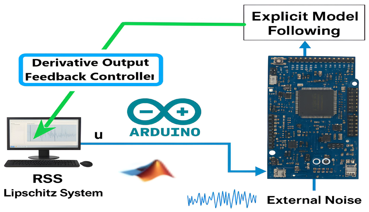
The experimental validation of the performance of the proposed approach was conducted with two examples using RTI, employing the ARDUINO DUE board as a real-time emulator. The RTI diagram is shown in Figure 1 (all technical implementation details are provided in [24] under the same conditions).

Figure 1. RTI diagram.

The RTI configuration shown in Figure 1 is implemented using an Arduino DUE board interfaced with MATLAB/Simulink R2023b in Input/Output mode.

To clarify the real-time procedure executed on the Arduino DUE, the following pseudo-code summarizes the control loop steps, as shown in Algorithm 1:

Algorithm 1 Pseudo-code of the EMF RTI

1: Initialization: Set sampling period $T_s=1$ ms; initialize states $\overline{x}\left(0\right)$, reference model $x_M\left(0\right)$, and control gain ${\Gamma }_y$. 2: while system is running do Acquire measurements $\overline{y}\left(t\right)$ from sensors. Compute derivative estimate $\dot{\overline{y}}\left(t\right)$ using filtered numerical differentiation. Evaluate control input $u\left(t\right)=-{\Gamma }_y\overline{y}\left(t\right)$. Apply $u\left(t\right)$ to the plant through the DAC output channel. Update model dynamics $x_M(t+T_s)$ and compute tracking error $\epsilon \left(t\right)={{\rm Y}}_M-{{\rm Y}}_F$. Log data for post-processing and performance evaluation. Wait until the next sampling instant: $t\leftarrow t+T_s$. 3: end while

This procedure corresponds to the Input/Output real-time communication loop between MATLAB/Simulink R2023b and the Arduino DUE board. Each iteration executes within approximately 0.42 ms, which is well below the sampling period, thereby ensuring real-time feasibility.

To minimize high-frequency noise during analog-to-digital conversion, LPF were applied to both the input and output channels of the Arduino DUE. Each LPF was implemented with a cut-off frequency of 50 Hz, which provides an efficient attenuation of measurement noise while preserving the dominant system dynamics (below 10 Hz). This filtering setup ensures accurate derivative estimation and stable closed-loop operation without significant phase delay.

Real-time experiments were conducted on an Arduino DUE microcontroller featuring an ARM Cortex-M3 processor running at 84 MHz with 96 KB of SRAM and 512 KB of flash memory. The analog input and output channels operate at 12-bit resolution. The EMF control algorithm was executed with a sampling frequency of 1 kHz (sampling period 1 ms), and the average execution latency per control cycle was approximately 0.42 ms, as measured using the Simulink Real-Time Toolbox. During the experiments, processor utilization remained below 65%, confirming that the proposed method satisfies the timing and computational constraints of low-cost embedded platforms.

A dedicated setup routine is employed to establish real-time communication between the plant emulator (system) and the host computer (model). The mathematical models of the nonlinear systems are inserted in the emulator through Embedded MATLAB Functions, ensuring efficient execution on the microcontroller. To improve signal quality, the input and output channels of the Arduino kit are filtered by low-pass filters, which suppress high-frequency noise and guarantee reliable data exchange. This setup provides a simple yet effective real-time environment to validate the proposed EMF control strategies.

4.1. Linear EMF

For the first example, the considered system is described as follows: $\overline{A}=\left[\begin{array}{cc}2.5& -2\\ 1.5& -2\end{array}\right]$; $\overline{B}=\left[\begin{array}{c}1\\ 0.5\end{array}\right]$; $\overline{\varphi }\left(\dot{x}\right)=\left[\begin{array}{c}0.25sin\left({\dot{x}}_1\left(t\right)\right)\\ 0\end{array}\right]$.

The chosen nonlinear benchmark system represents a simplified electromechanical setup in which the sinusoidal term $0.25sin\left({\dot{x}}_1\left(t\right)\right)$ emulates a bounded actuator nonlinearity. Such sinusoidal perturbations are commonly encountered in servo drives, DC motor mechanisms, and electromechanical actuators, as reported in [11,16]. The selected Lipschitz constant ${\theta }_{\phi }=0.25$ reflects a moderate nonlinearity level, ensuring realistic dynamic behavior while maintaining analytical tractability and reproducibility in RTI.

Then, the open-loop poles of the system are located at $1.6861$ and $-1.1861$. As a result, the system is unstable and will diverge from any non-zero initial condition unless it is properly controlled (from (13), ${\overline{x}}_0^T=\left[\begin{array}{cccc}0.8& 0.8& 0.7& 0.7\end{array}\right]$).

Suppose that the matrices of the desired model specified in (8) are chosen as follows: ${\overline{A}}_M=\left[\begin{array}{cc}-1& 2\\ -1.5& -1\end{array}\right]$; ${\overline{C}}_M=I_2$; ${\overline{{\rm Y}}}_F={\overline{{\rm Y}}}_M=\left[\begin{array}{cc}0.9& 0.4\end{array}\right]$.

• Note that the system poles of the desired model are at $-1\pm 1.732i$. The weighting matrices in (19) are selected as follows: $\overline{Q}=0.2$ and $\overline{R}=0.03$.

The weighting matrices $Q=0.2$ and $R=0.03$ were tuned according to a normalized energy tradeoff principle, where Q penalizes the model-tracking error, and R penalizes the control effort. This balance ensures smooth control action while maintaining accurate tracking. Increasing Q tends to accelerate convergence but may introduce oscillations, whereas increasing R smooths the control at the expense of slower dynamics. Sensitivity analysis showed that the closed-loop stability and asymptotic tracking properties remain robust for $Q\in [0.1,0.5]$ and $R\in [0.01,0.1]$, demonstrating the flexibility of the proposed EMF design for other nonlinear systems. Subsequently, the resolutions of (9) give the following control parameters:

$${\overline{\Gamma }}_y=\left[\begin{array}{cccc}5.7062& -2.3758& -1.7801& -1.8784\end{array}\right]$$

$$\overline{P}=\left[\begin{array}{cccc}0.845& 0.7307& 0.6775& 0.6772\\ ★& 0.7221& 0.6628& 0.6694\\ ★& ★& 0.6811& 0.6705\\ ★& ★& ★& 0.6844\end{array}\right]$$

$$\overline{U}=\left[\begin{array}{cccc}0.0891& -0.034& -0.047& -0.0469\\ ★& 0.071& -0.0235& -0.034\\ ★& ★& 0.0303& -0.0417\\ ★& ★& ★& 0.0469\end{array}\right]$$

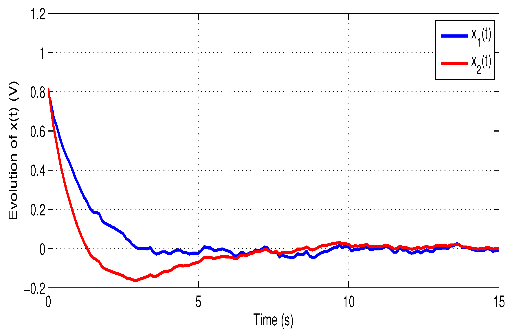
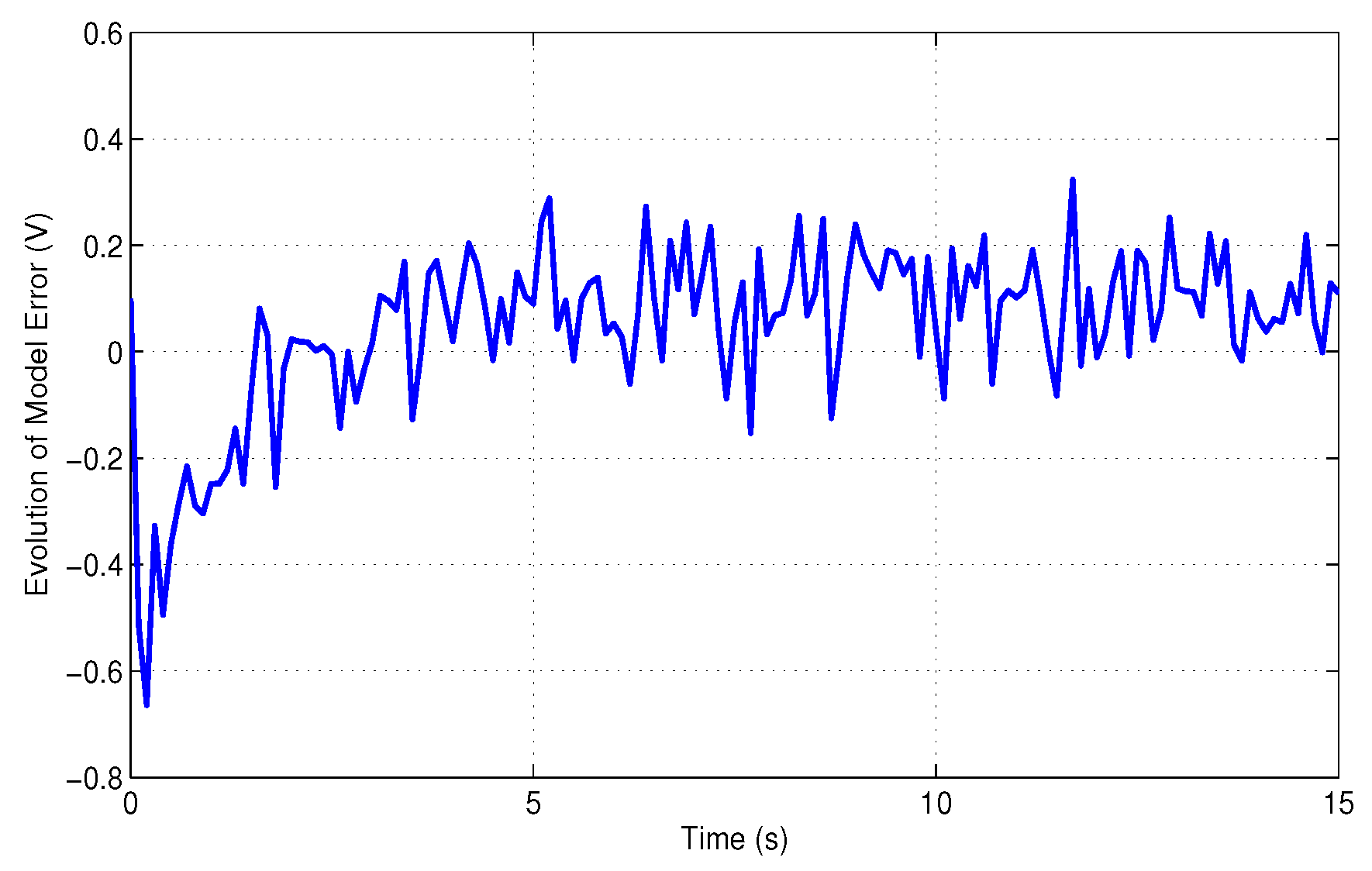
Now, Figure 2 and Figure 3 plot the evolution of states in the closed-loop system and the error dynamics between the system and model performance outputs:

Figure 2. The evolution of states $\overline{x}\left(t\right)$ under the proposed EMF controller.

Figure 3. Variation in error dynamics between system and model’s performance outputs.

According to the results presented in Figure 2 and Figure 3, it is evident that the states achieve asymptotic stability, with the model error converging to 0.

4.2. Nonlinear EMF

In this part, the same example as in the previous section is considered such that the desired nonlinear function is as follows:

$${\overline{\varphi }}_M\left(\dot{x}\right)=\left[\begin{array}{c}3.33sin\left({\dot{x}}_1\left(t\right)\right)\\ 0\end{array}\right]$$

This choice of nonlinear function is designed to evaluate a critical case: that of systems characterized by a high Lipschitz constant (that of the real system is $0.25$, and that of the desired model is $3.33$, more than 10 times greater). Now, solving (36) gives the following:

$${\overline{\Gamma }}_y=\left[\begin{array}{cccc}15.19& -3.09& 0.11& 0.83\end{array}\right]$$

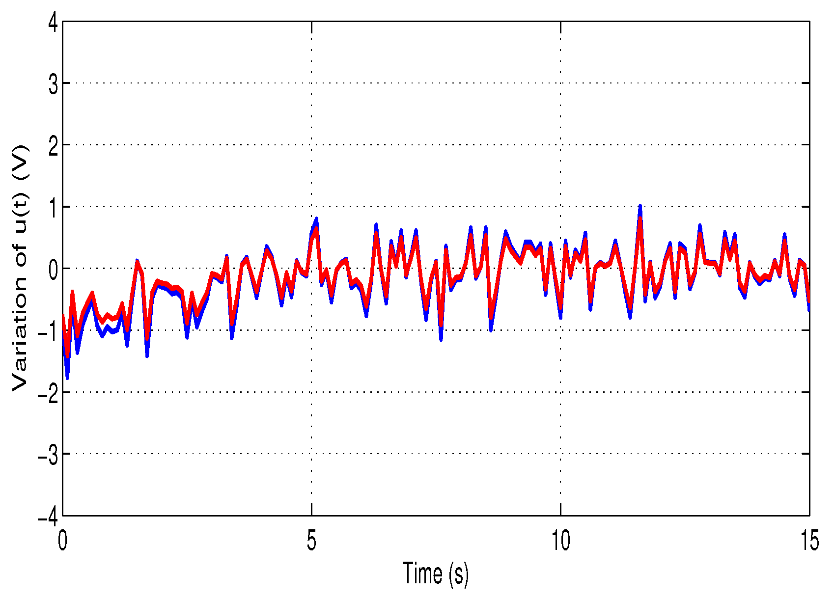
First, Figure 4 illustrates the progression of the control $\overline{u}\left(t\right)$:

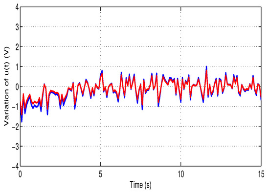
Figure 4. Control $\overline{u}\left(t\right)$ variation for NEMF (${\overline{u}}_1\left(t\right)$)-blue and ${\overline{u}}_2\left(t\right)$-red.

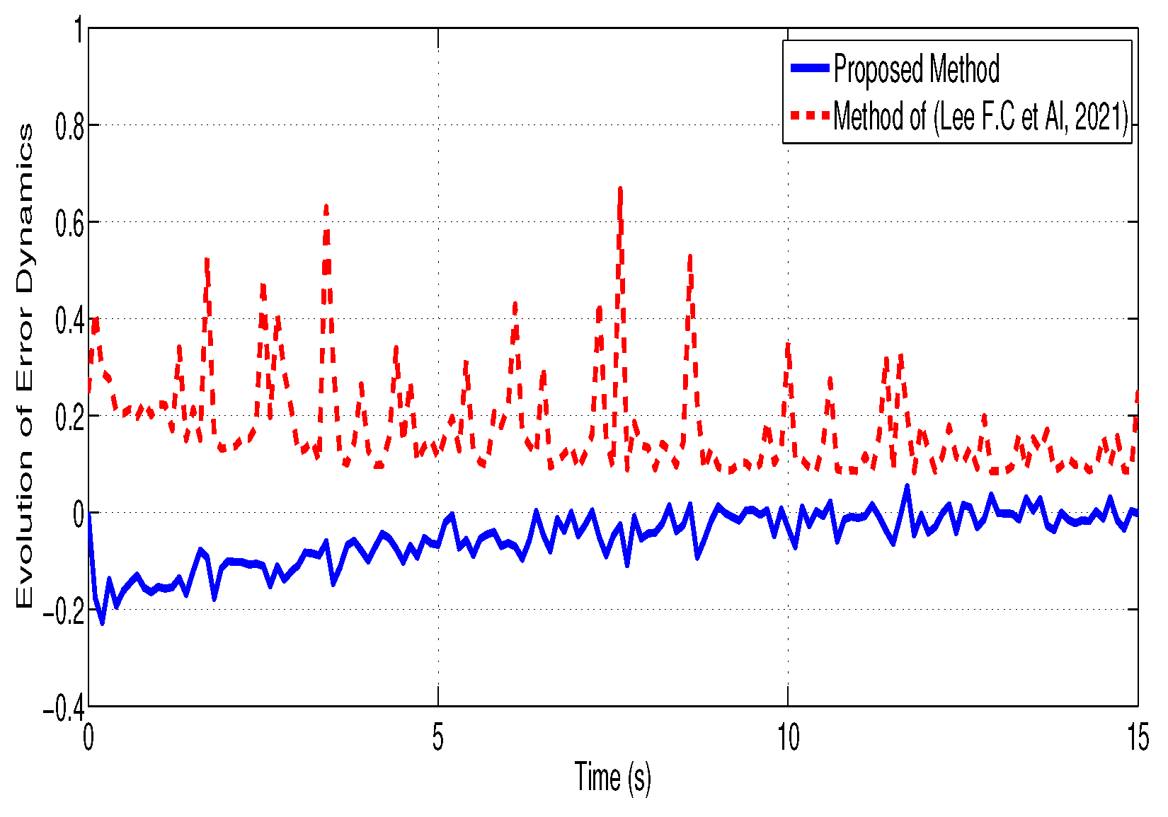
In Figure 5, the behavior of the error dynamics is presented, contrasting the model’s performance with that of [16] when the Lipschitz constant is raised to ${\theta }_{\phi }=5.25$.

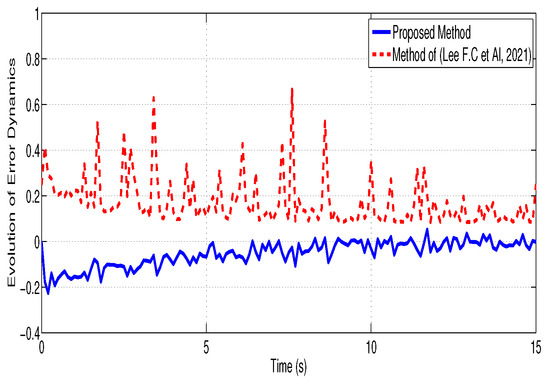
Figure 5. Evolution of error dynamics under proposed EMF controller and [16].

Figure 4 and Figure 5 reveal that the proposed EMF control law ensures the stability of the overall system, exhibiting minimal disturbances and reduced amplitude fluctuations, unlike the method from [16], which produces biased results.

From Figure 2, Figure 3, Figure 4 and Figure 5, the closed-loop states exhibit asymptotic convergence with an average decay rate of approximately 0.8 ${\mathrm{s}}^{-1}$. The steady-state tracking error norm satisfies $\parallel \epsilon \left(t\right)\parallel <0.05\mathrm{V}$ after 6 s, confirming precise alignment between the system and model outputs. Compared to the reference method in [16], the proposed EMF controller achieves a reduction of about 35% in overshoot and oscillation amplitude, leading to smoother transients and improved steady-state stability. These quantitative observations substantiate the qualitative claim of reduced oscillations and enhanced performance robustness.

Furthermore, Table 1 summarizes key quantitative performance indices obtained from the real-time experiments. For the proposed linear EMF controller, the steady-state tracking error satisfies ${\parallel \epsilon \left(t\right)\parallel }_{\infty }<0.05\mathrm{V}$ with a mean settling time of approximately 4.7 s, whereas the method reported in [16] requires about 7.2 s under the same conditions. The maximum overshoot is reduced by nearly 35%, and the control effort (RMS value of $u\left(t\right)$) decreases by 22% in the nonlinear EMF configuration. These results confirm that the proposed approach provides faster convergence, smaller oscillations, and lower control energy than the reference method.

Table 1. Quantitative performance comparison between proposed EMF method and [16].

Metric	Proposed EMF	Method [16]	Improvement (%)
Settling time (s)	4.7	7.2	34.7
Max. overshoot (%)	8.1	12.5	35.2
Steady-state error (V)	<0.05	0.08	37.5
Control RMS (V)	0.62	0.80	22.5

Discussion on Experimental Outcomes:

The experimental results demonstrate clear alignment between theoretical predictions and real-time performance. As shown in Figure 2, Figure 3, Figure 4 and Figure 5, both the system states and the tracking error exhibit smooth transient behavior, confirming the asymptotic stability guaranteed by the LQR-based design. The reduced oscillations in the control input reflect the damping effect introduced by the weighting matrix R, while the fast convergence of the model error highlights the efficiency of the derivative-based feedback in compensating nonlinearities. Furthermore, the nonlinear EMF controller maintains robustness under variations in the Lipschitz constant, indicating that the proposed design preserves stability margins even when the system operates beyond nominal conditions. Overall, these results validate the practical effectiveness of the EMF framework and bridge the gap between mathematical derivations and embedded implementation outcomes.

Note: It should be emphasized that real-time validation was intentionally performed on low-order benchmark systems to ensure computational feasibility on the Arduino DUE microcontroller. This hardware limitation does not restrict the generality of the proposed EMF approach, which remains theoretically applicable to higher-order LNSs. Extending the method to large-scale or high-dimensional systems would mainly involve optimizing the numerical solution of the algebraic equations and, if necessary, developing distributed or hierarchical implementations to preserve real-time performance. This extension will be considered in future work.

5. Conclusions

In this paper, an EMF control strategy for LNS in RSS form was presented, using derivative output feedback. By exploiting the DMVT, the nonlinear system was reformulated as an LPV representation, which simplifies the control design. The synthesis relies on an LQR-based gain computation, combined with Lipschitz conditions and supporting lemmas, to guarantee the asymptotic stability of the closed-loop system.

Experimental validation on an Arduino DUE platform demonstrated the effectiveness of the proposed approach in stabilizing nonlinear plants subject to perturbations and nonlinearities. Both the linear and nonlinear EMF designs showed satisfactory tracking performance and robustness, even in the presence of higher Lipschitz constants.

Although the validation focused on low-order benchmark systems to ensure feasibility in a real-time embedded environment, the proposed methodology is general and applicable to higher-order LNS.

Future research will focus on extending the proposed EMF control framework to large-scale and high-order LNS. This extension will address computational scalability and coupling effects among interconnected subsystems, possibly through decentralized or hierarchical architectures. Another research direction concerns robustness analysis with respect to parametric uncertainties and external perturbations, where $H_{\infty }$-based formulations and LMI relaxations can be incorporated to enhance stability margins. Moreover, developing nonlinear output feedback EMF strategies is expected to improve the applicability of the method in complex cyber-physical systems subject to communication constraints and measurement imperfections.

References

- Wang, Y.; Duan, G.; Li, P. Event-Triggered Adaptive Sliding Mode Control of Uncertain Nonlinear Systems Based on Fully Actuated System Approach. IEEE Trans. Circuits Syst. II Express Briefs 2024, 71, 2749–2753. [Google Scholar] [CrossRef]
- Xiao, W.X.; Jiang, G.R.; Mao, J.K.; Xie, F.; Zhang, B.; Qiu, D.Y.; Chen, Y.F. Adaptive Logarithmic State Feedback Control with Quasi One-Switching-Cycle Response Characteristic for Three-Phase Inverter. IEEE Trans. Circuits Syst. II Express Briefs 2024, 71, 3046–3050. [Google Scholar] [CrossRef]
- Keel, L.H.; Bhattacharyya, S.P. New Conditions for the Stability and Instability of Feedback Systems. In Proceedings of the IECON 2021—47th Annual Conference of the IEEE Industrial Electronics Society, Toronto, ON, Canada, 13–16 October 2021; pp. 1–5. [Google Scholar] [CrossRef]
- Yu, G.R. Explicit Model-Following Design of Propulsion Control Aircraft Using Genetic Algorithms. In Proceedings of the 2006 IEEE International Conference on Systems, Man and Cybernetics, Taipei, Taiwan, 8–11 October 2006; pp. 4348–4353. [Google Scholar] [CrossRef]
- Metzler, M.; Tavernini, D.; Gruber, P.; Sorniotti, A. On Prediction Model Fidelity in Explicit Nonlinear Model Predictive Vehicle Stability Control. IEEE Trans. Control Syst. Technol. 2021, 29, 1964–1980. [Google Scholar] [CrossRef]
- Hou, Z.; Xiong, S. On Model-Free Adaptive Control and Its Stability Analysis. IEEE Trans. Autom. Control 2019, 64, 4555–4569. [Google Scholar] [CrossRef]
- Zhang, J.X.; Li, K.W.; Li, Y.M. Output-Feedback Based Simplified Optimized Backstepping Control for Strict-Feedback Systems with Input and State Constraints. IEEE/CAA J. Autom. Sin. 2021, 8, 1119–1132. [Google Scholar] [CrossRef]
- Xu, J.; Bhattacharyya, S.P. Efficient Tuning of PID Controllers using Swarm-based Optimization Algorithms. In Proceedings of the 2021 9th International Conference on Systems and Control (ICSC), Caen, France, 4–26 November 2021; pp. 572–579. [Google Scholar] [CrossRef]
- Thabet, A.; Gasmi, N.; Bel Haj Frej, G. Robust state and output feedback stabilization for Lipschitz nonlinear systems in reciprocal state space: Design and real-time validation. Proc. Inst. Mech. Eng. Part I J. Syst. Control Eng. 2024, 238, 1296–1306. [Google Scholar] [CrossRef]
- Tseng, Y.W.; Wang, Y. Model following variable structure control design in reciprocal state space framework with dead-zone nonlinearity and lumped uncertainty. In Proceedings of the 7th IEEE Conf. on Industrial Electronics and Applications, Singapore, 18–20 July 2012; pp. 1627–1632. [Google Scholar] [CrossRef]
- Kaewpraek, N.; Assawinchaichote, W. H∞ fuzzy state-feedback control plus state-derivative-feedback control synthesis for photovoltaic systems. Asian J. Control 2016, 18, 1441–1452. [Google Scholar] [CrossRef]
- Tseng, Y. Control design for system with lipschitz nonlinearity of state derivative variables in reciprocal state space form. In Proceedings of the International Conference on Image Processing, Electronics and Computer Engineering, Singapore, 8–9 July 2015; pp. 26–32. [Google Scholar]
- Thabet, A. Adaptive-state feedback control for lipschitz nonlinear systems in reciprocal-state space: Design and experimental results. Proc. Inst. Mech. Eng. Part I J. Syst. Control Eng. 2019, 233, 144–152. [Google Scholar] [CrossRef]
- Sever, M.; Yazici, H. LMI-based designs for robust state and output derivative feedback guaranteed cost controllers in reciprocal state space form. Int. J. Control 2019, 94, 2224–2237. [Google Scholar] [CrossRef]
- Tseng, Y. Sliding mode control with state derivative feedback in novel reciprocal state space form. Adv. Appl. Nonlinear Control Syst. 2016, 635, 159–184. [Google Scholar]
- Lee, F.C.; Tseng, Y.; Wu, R.C.; Chen, W.C.; Chen, C.S. Inverse Optimal Control in State Derivative Space System with Applications in Motor Control. Energies 2021, 14, 1775. [Google Scholar] [CrossRef]
- Thabet, A.; Gasmi, N.; Frej, G.B.H.; Boutayeb, M. Sliding Mode Control for Lipschitz Nonlinear Systems in Reciprocal State Space: Synthesis and Experimental Validation. IEEE Trans. Circuits Syst. II Express Briefs 2021, 68, 948–952. [Google Scholar] [CrossRef]
- Tseng, Y.W.; Hsieh, J.G. Optimal Control for a Family of Systems in Novel State Derivative Space Form with Experiment in a Double Inverted Pendulum System. Abstr. Appl. Anal. 2013, 2013, 715026. [Google Scholar] [CrossRef]
- Nosrati, K.; Belikov, J.; Tepljakov, A.; Petlenkov, E. Revisiting the LQR problem of singular systems. IEEE/CAA J. Autom. Sin. 2024, 11, 2236–2252. [Google Scholar] [CrossRef]
- Yazici, H.; Sever, M. L2 gain state derivative feedback control of uncertain vehicle suspension systems. J. Vib. Control 2018, 24, 3779–3794. [Google Scholar] [CrossRef]
- Tseng, Y.W.; Wu, R.C. Model-Following Designs Using Direct State Derivative Measurement Feedback in Novel Reciprocal State Space Form. J. Appl. Math. Phys. 2019, 7, 394–409. [Google Scholar] [CrossRef]
- Zemouche, A.; Boutayeb, M. On LMI conditions to design observers for Lipschitz nonlinear systems. Automatica 2013, 49, 585–591. [Google Scholar] [CrossRef]
- Zemouche, A.; Rajamani, R.; Phanomchoeng, G.h.; Boulkroune, B.; Rafaralahy, H.; Zasadzinski, M. Circle criterion-based H∞ observer design for Lipschitz and monotonic nonlinear systems-Enhanced LMI conditions and constructive discussions. Automatica 2017, 85, 412–425. [Google Scholar] [CrossRef]
- Gasmi, N.; Boutayeb, M.; Thabet, A.; Aoun, M. Sliding window based nonlinear H∞ filtering: Design and experimental results. IEEE Trans. Circuits Syst. II Express Briefs 2019, 66, 302–306. [Google Scholar] [CrossRef]
- Liu, D.; Zhang, G.; Xie, Y. Guaranteed Cost Control for a Class of Descriptor Systems with Uncertainties. Int. J. Inf. Syst. Sci. 2009, 5, 430–435. [Google Scholar]
Disclaimer/Publisher’s Note: The statements, opinions and data contained in all publications are solely those of the individual author(s) and contributor(s) and not of MDPI and/or the editor(s). MDPI and/or the editor(s) disclaim responsibility for any injury to people or property resulting from any ideas, methods, instructions or products referred to in the content. |
© 2025 by the authors. Licensee MDPI, Basel, Switzerland. This article is an open access article distributed under the terms and conditions of the Creative Commons Attribution (CC BY) license (https://creativecommons.org/licenses/by/4.0/).