Abstract
In the context of climate change and energy transition, the growing frequency of extreme weather events threatens the safety and stability of power systems. Given the limitations of existing research on load characteristic analysis and load forecasting during extreme weather events, this paper proposes a load-integrated forecasting model that accounts for extreme weather. First, an improved power load clustering method is proposed, combining Kernel PCA for nonlinear dimensionality reduction and an enhanced k-means algorithm, enabling both qualitative analysis and quantitative representation of load characteristics under extreme weather. Second, an optimal combination forecasting model is developed, integrating improved SVM and enhanced LSTM networks. Building upon the improved power load clustering algorithm, a load-integrated forecasting model considering extreme weather is established. Finally, based on the proposed load-integrated forecasting model, a time-series production simulation model considering extreme weather is constructed to quantitatively analyze the power and electricity balance risks of the system. Case studies demonstrate that the proposed integrated forecasting model can effectively analyze load characteristics under extreme weather and achieve more accurate load forecasting, which can provide guidance for the planning and operation of new power systems under extreme weather conditions.
1. Introduction
Climate change and energy transition have been focal points of domestic and international attention. The large-scale exploitation and utilization of fossil fuels have led to a series of issues, including severe environmental pollution, energy resource shortages, and frequent extreme weather events, which will impose significant economic losses and safety risks on human society. Currently, countries worldwide are promoting green transitions and building clean, low-carbon energy structures.
In recent years, as global climate change intensifies, the frequency of extreme weather events has risen significantly. In 2021, Texas, USA, experienced extreme cold weather, leading to supply–demand imbalances and blackouts [1]. In 2022, Sichuan, China, faced extreme high temperatures, resulting in a sharp decline in hydropower generation and a surge in load demand, triggering large-scale severe power rationing [2]. In 2023, Northeast China encountered heavy rainfall and extreme cold weather, causing widespread outages at substations, transmission lines, and power consumers [3]. Moreover, the quantity and variety of power loads have undergone exponential growth alongside the development of modern power systems. The increasing proportion of renewable energy further exacerbates the volatility and uncertainty on the load side. Therefore, in the face of these challenges, conducting research on load characteristics under extreme weather conditions is imperative for ensuring the secure and stable operation of modern power systems.
Load characteristic analysis refers to the analysis of the electricity consumption behavior and characteristics of loads in power systems. This analysis offers guidance for load forecasting and grid planning, helping achieve supply–demand balance.
Load characteristic indicators help analyze the intrinsic features of load curves and reveal the patterns of load behavior. Reference [4] selects typical indicators such as maximum load utilization hours, peak–valley load differences, and load factors to analyze load curves based on load variations across different time scales. Reference [5] proposes three indicators—day–night electricity consumption differences, daily load factors, and peak–valley difference rates. Reference [6] introduces key indicators such as peak–valley load ratios, cooling-to-electricity ratios, and peak–valley difference rates to extract load characteristics.
Regarding load characteristic analysis methods, researchers worldwide have conducted extensive studies on clustering-based approaches. Reference [7] employs the fuzzy C-means clustering method to cluster daily load curves, demonstrating that this method can effectively reflect load consumption characteristics. Reference [8] adopts the K-medoids clustering algorithm for load characteristic analysis, using the obtained cluster centers as typical load curves. References [9,10] apply the k-means clustering method to classify and analyze load characteristic curves. Reference [11] proposes a spectral clustering method based on information entropy and correlation measurement for clustering analysis. Reference [12] uses the ISODATA algorithm to extract typical user categories from massive load data. Reference [13] proposes a portrait-based method for assessing the demand response potential of industrial parks. That study conducts load characteristic analysis using hierarchical clustering and k-means clustering and classifies and summarizes the typical electricity consumption behaviors of loads. Reference [14] employs a heuristic algorithm to enhance the performance of traditional clustering algorithms to a certain extent. Given the high dimensionality of load data, dimensionality reduction techniques can further improve clustering performance and computational efficiency [15]. Reference [16] proposes a power load curve clustering method incorporating PCA dimensionality reduction that enhances computational efficiency and clustering accuracy. However, linear dimensionality reduction algorithms struggle to adapt to nonlinear load clustering scenarios. Reference [17], based on a deep learning clustering method, adopts a self-organizing mapping approach for load clustering, which effectively improves the clustering effect.
Load forecasting is a critical basis for the safe and economic operation of power systems. Scholars worldwide have carried out extensive studies on traditional and modern load forecasting methods. References [18,19] use multiple linear regression and exponential smoothing methods for load forecasting, respectively, but it is difficult to maintain good prediction accuracy when there are large fluctuations in the load. Reference [20] employs a BP neural network combined with kernel density estimation for load forecasting, designing an ultra-short-term power load forecasting model based on a randomly distributed embedded framework that incorporates regional load data from Australia, meteorological parameters including dry-bulb temperature and wet-bulb temperature, and holiday information with meteorological data integrated as delay variables to achieve accurate forecasting in extreme weather scenarios. Reference [21] utilizes a support vector machine (SVM) model for load forecasting, demonstrating superior performance compared to traditional models. Reference [22] adopts a deep learning model based on Deep Belief Networks (DBNs) to extract complex features from data for accurate load forecasting. To overcome the limitations of recurrent neural networks, reference [23] applies Long Short-Term Memory (LSTM) networks to capture long-term dependencies in load sequences. Reference [24] proposes an improved deep learning model for short-term load forecasting. It utilizes random forest for feature selection and incorporates rough set theory to correct prediction results, substantially enhancing the forecasting accuracy. The Transformer model was originally proposed by Google in 2017 and has since been widely adopted in load forecasting by many researchers. Reference [25] presented an improved Transformer-based method for power load forecasting that deeply integrates the position, trend, periodicity, and weather information of load sequences, effectively capturing long-term dependencies in temporal load data.
Additionally, some studies combine multiple models to further improve forecasting accuracy. Reference [26] employs Variational Mode Decomposition combined with a bidirectional LSTM network for load forecasting, establishing a short-term power load forecasting model that integrates DBO-VMD with the IWOA-BILSTM neural network. This model processes actual grid load data from March to May 2012, where DBO-VMD decomposition reduces load data volatility, and the IWOA-optimized bidirectional LSTM enables accurate prediction of load components, effectively mitigating errors caused by load fluctuations. Reference [27] proposes a combined forecasting method based on the improved golden jackal algorithm and the LSTM network. This method processes regional load data from Henan along with meteorological variables, such as maximum, minimum, and average temperature and relative humidity, and optimizes LSTM hyperparameters through the improved algorithm to significantly enhance prediction accuracy and stability. Reference [28] leverages the strengths of both the BP and RBF neural networks to achieve nonlinear fitting and rapid, accurate load forecasting. Reference [29] constructs a combined load forecasting model by integrating multiple linear regression and temporal convolutional networks and verifies the accuracy of this method through analysis. Since power load is affected by various factors, fully considering the influencing factors of load characteristics is helpful to improve the performance of load forecasting models [30]. Reference [31] proposes a short-term load forecasting method utilizing meteorological data dimensionality reduction and hybrid deep learning. The approach inputs regional load data and seven-dimensional meteorological parameters, including temperature, humidity, and wind speed; reduces data dimensionality through sparse kernel principal component analysis; and constructs a CNN-LSTM hybrid model to achieve accurate load forecasting. Reference [32] builds a combined forecasting model based on LSTM and multi-task learning, which effectively improves the accuracy of multi-variable load forecasting. Reference [33] proposed the MSTGCN-T model, which employs a multi-scale spatiotemporal graph convolutional network to capture short-term spatiotemporal features among nodes and integrates Transformer to model long-term temporal dependencies, significantly improving the accuracy and stability of load forecasting.
Currently, most studies only consider load forecasting under normal weather conditions, while a small number of scholars have taken the impact of special situations, such as extreme weather, into account when conducting power load forecasting. Reference [34] considers different special events, including the Spring Festival period, major political events, and extreme weather. Based on the results of load decomposition, it establishes an ARIMA model for the deterministic load component, an LSSVM model for the periodic load component, and an LSTM model for the random load component. Through this approach, a combined forecasting model is constructed to achieve an accurate prediction of power load during special events. Reference [35] divides the dataset into four weather types. It calculates the correlation coefficients between meteorological factors and power load under various weather conditions and conducts cluster analysis on the influencing factors with the highest correlation. This process yields refined datasets with higher similarity, and load forecasting results are obtained based on the CNN model. Reference [36] screens out extreme high-temperature weather based on temperature and heat indices. It uses a tensor low-rank completion algorithm to supplement missing data under extreme weather and realizes load forecasting under extreme high-temperature weather through Pearson correlation analysis and the LSTM model. However, a notable research gap remains in the selection and efficacy of specific climatic variables as model inputs for extreme weather conditions. The exploration of composite indices—such as apparent temperature, wet-bulb temperature, or the wind chill index—which may more accurately represent the human-perceived weather severity and its subsequent impact on electricity demand, is still insufficient. Systematically evaluating and comparing these variables’ predictive power could be a crucial direction for future work.
In summary, existing research on load characteristic analysis mainly focuses on load curve clustering and influencing factors, with relatively limited studies considering extreme weather conditions. Meanwhile, clustering-based load characteristic analysis methods still require improvements in computational accuracy and efficiency. In terms of load forecasting, existing research lacks sufficient attention to load forecasting under extreme weather conditions. Therefore, it is necessary to establish efficient and accurate load characteristic analysis methods under extreme weather and conduct comprehensive analyses of load characteristics in such scenarios. Additionally, load forecasting should incorporate extreme weather and other influencing factors to achieve more accurate predictions.
The main contributions put forward in this paper can be summarized as follows:
- An improved power load clustering method based on the KPCA nonlinear dimensionality reduction method and the improved K-means algorithm is proposed. The effectiveness of the algorithm is evaluated based on multiple indicators, providing algorithmic support for power load forecasting under extreme weather conditions.
- An improved PSO algorithm based on the golden sine is proposed to optimize the hyperparameters of the prediction model. An optimal combination forecasting model is constructed using the improved SVM algorithm and the improved LSTM algorithm. Based on the improved power load clustering algorithm proposed in this paper, a load-integrated forecasting model considering extreme weather is built to achieve more accurate load forecasting results.
- Based on the load-integrated forecasting model, a time-series production simulation model considering extreme weather is constructed to evaluate the operation status of the power system, providing guidance for the planning and construction of the system under extreme conditions.
2. Power Load Characteristic Analysis Methods Under Extreme Weather
2.1. Construction of Multi-Dimensional Power Load Characteristic Indicators
To accurately describe the time-varying characteristics of power loads under extreme weather conditions, this section proposes multi-dimensional power load characteristic indicators and establishes an indicator system that can comprehensively reflect power load characteristics under extreme weather in two dimensions: statistical characteristics and shape characteristics. The specific indicators are shown in Figure 1. The specific explanations of the power load characteristic indicators are as follows:
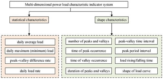
Figure 1.
Multi-dimensional power load characteristic indicator system.
- 1.
- Statistical Characteristic Analysis
- Daily average load: This is calculated by dividing the daily electricity consumption by 24 h or taking the average value of the load in each time period within a day.
- Daily maximum (minimum) load: This refers to the maximum (minimum) load values recorded in the load data of a typical day.
- Peak–valley difference rate: This is the ratio of the difference between the daily maximum and minimum loads to the maximum load.
- Daily load rate: This is the ratio of the daily average load to the daily maximum load among the loads recorded on a typical day. This indicator can effectively reflect the balance degree of load distribution throughout the day. The formula is
- 2.
- Shape Characteristic Analysis
- Number of peaks and valleys: The number of peak points and valley points in the power load curve during a specific statistical period.
- Time of peaks and valleys occurrence: The time corresponding to the maximum load and minimum load point in the power load curve during a specific statistical period.
- Duration of peaks and valleys: The duration corresponding to each load peak period and each load valley period in the power load curve during a specific statistical period.
- Peak–valley time interval: During a specific statistical period, the shortest time interval between adjacent load peaks and valleys is the peak–valley time interval.
- Peak period interval: During a specific statistical period, the shortest time interval between these peaks is the peak period interval.
- Load rising time and falling time: The power load rising time refers to the time taken for the load to rise from 1.3 times the base load to 0.6 times the peak load; the power load falling time refers to the time taken for the load to drop from 0.6 times the peak load to 1.3 times the base load. A schematic diagram of the electrical load rising time and falling time is shown in Figure 2. In this figure, and represent the daily maximum load and daily minimum load, respectively.
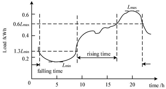 Figure 2. Schematic diagram of the rising time and falling time of an electrical load.
 - Shape of load curve: The daily load curve depicts the hourly load variation trajectory within a day, which can clearly show the dynamic change trend of the load over time, including valley-filling type, the double-peak and double-valley type, and the continuous or single-peak type.
2.2. Load Curve Clustering Method Under Extreme Weather
Most existing load characteristic analyses focus on clustering algorithms, while traditional load curve clustering methods rarely consider load variation trends under extreme weather conditions. This section studies the analysis method for power load characteristics under extreme weather conditions and proposes a load curve clustering analysis method based on dimensionality reduction technology and improved k-means. It improves the shortcomings of traditional algorithms to accurately explore the power system load characteristics under extreme weather conditions.
2.2.1. Power Load Dimensionality Reduction Method Based on KPCA
A power load usually has nonlinear characteristics and high dimensionality. Therefore, it is essential to choose a suitable method for reducing the dimensionality of load data that can also handle the nonlinear characteristics of power loads well. As a nonlinear dimensionality reduction method, KPCA (kernel principal component analysis) can effectively capture the nonlinear relationships in load data and retain global features, which is more in line with the laws of load data compared with traditional PCA.
The core idea of the KPCA method is to use kernel functions to implicitly calculate the inner product in high-dimensional space, avoiding explicit high-dimensional mapping, thereby efficiently capturing the nonlinear structure of data. Suppose the input space, , contains n samples, . A certain nonlinear mapping function, , is used to map the data to the high-dimensional space, . If in all samples , the kernel function can be expressed by the dot product of the nonlinear mapping function:
where is the kernel function between sample and sample . The commonly used kernel functions mainly include the following types:
- 1.
- Linear Kernel
- 2.
- Polynomial Kernel
- 3.
- Gaussian Kernel
The Gaussian kernel function can deal with more complex nonlinear relationships and has good adaptability, flexibility, and anti-interference abilities in cases such as extreme weather. Therefore, the Gaussian kernel function is adopted for the dimensionality reduction in power load data.
The detailed process of the power load dimensionality reduction method based on KPCA is shown in Algorithm 1.
| Algorithm 1. Power load dimensionality reduction method based on KPCA. |
| Input: Original load data |
| Output: Load data after dimensionality reduction |
|
|
|
|
|
2.2.2. Improved K-Means Method for Power Load Clustering
Under extreme weather conditions, power load changes exhibit significant nonlinearity, abruptness, and diversity. Traditional load classification and clustering methods, including the widely used K-means algorithm for extracting typical load curves, fuzzy C-means for reflecting consumption characteristics, and K-medoids for identifying cluster centers, struggle to effectively analyze power load characteristics under extreme weather. Therefore, on the basis of combining nonlinear dimensionality reduction strategies, it is necessary to make relevant improvements to traditional methods to more precisely and accurately identify typical load consumption patterns under extreme weather and realize the qualitative analysis of load characteristics under extreme weather.
K-means is a partitioning-based clustering algorithm that divides data into K clusters, , by minimizing the sum of squared Euclidean distances between samples and cluster centers. The calculation steps are as follows:
- 1.
- Initialize cluster centers: Randomly select K samples as initial cluster centers. .
- 2.
- Sample assignment: Calculate the distance from each sample to each cluster center, and assign it to the nearest cluster:
- 3.
- Update cluster centers: Recalculate the mean of each cluster as the new cluster center:
- 4.
- Repeat steps 2–3, and the algorithm terminates when the cluster centers converge or the maximum iteration count is satisfied.
The traditional k-means algorithm has strong interpretability and low complexity, but it is prone to falling into local optimal solutions, resulting in poor clustering effects. To address the shortcomings of traditional clustering algorithms and enhance the global search capabilities of the algorithm, this paper introduces probability weights to optimize the selection of initial cluster centers and combines clustering validity indices with the global convergence advantages of the improved PSO algorithm based on golden sine to find the optimal number of clusters for the k-means algorithm. This can ensure computational efficiency while obtaining more accurate and reliable load clustering results under extreme weather conditions.
- Optimization of initial cluster center selection
The initial centers are selected through probability weights to make the distribution of center points more uniform:
where is the probability weight that sample is selected as the next cluster center.
- Determination of optimal number of clusters
The silhouette coefficient index for sample i is defined as
where is the average intra-cluster distance, and is the minimum average inter-cluster distance.
The mean SC of all sample in the dataset is used as the validity index for the overall clustering effect of the algorithm. A larger SC indicates better clustering quality.
- Improved PSO Algorithm Based on Golden Sine
The PSO algorithm is introduced to dynamically adjust the number of clusters and avoid local optima. To balance convergence speed and search accuracy, a dynamically adjusted inertia weight, , is incorporated. Furthermore, this paper introduces the golden sine algorithm during the optimization process, which has strong global search capabilities. By integrating the golden section coefficient into the position update process, it can appropriately balance the global search and local optimization capabilities of the algorithm, thereby improving the algorithm’s performance.
A velocity update formula with dynamic inertia weight is introduced:
where and , respectively, represent the velocity and position of the i-th particle in the j-th dimension during the t-th iteration; pebst denotes the individual optimal solution of each particle, and gbest denotes the global optimal solution of the entire population; and are learning factors, usually ; rand is a random number between 0 and 1; is the inertia weight during the t-th iteration; and are the maximum and minimum inertia weight, respectively; and is the maximum number of iterations.
The particle position update formula based on the golden sine algorithm is
where is a random number between [0, 2π]; is a random number between [0, π]; and are coefficients obtained by the golden section method, which can reduce the search space; and is the golden section number, with a value of .
- Clustering performance evaluation index
The DBI (Davies–Bouldin index) is an evaluation indicator based on the ratio of inter-cluster and intra-cluster distances. If the similarity between clusters is higher (i.e., the DBI index is relatively high), it indicates that the distance between clusters is smaller, and thus, the clustering result is poorer. Therefore, a smaller DBI indicates a better clustering effect. Its expression is
where both and represent the sum of the average distances from all points within a cluster to the cluster center, and represents the clustering between two clusters.
The CHI (Calinski–Harabasz index) is an evaluation indicator based on the ratio of between-cluster variance to within-cluster variance. This indicator value can be expressed as the ratio of separation to compactness, so a larger value indicates a better result. The expression of the CHI index is
where represents the covariance matrix of the inter-cluster data; represents the covariance matrix of intra-cluster data; and and represent the trace of the intra-cluster scatter matrix and the trace of the inter-cluster scatter matrix, respectively.
The power load clustering method based on KPCA dimensionality reduction and an improved k-means algorithm proposed in this section can specifically analyze the impact of power load data dimensions, the selection of initial cluster centers, and the number of clusters on the load curve clustering results and more accurately identify typical load patterns under extreme weather conditions.
3. Construction of Load-Integrated Forecasting Model Considering Extreme Weather
3.1. Feature Selection Processing
There are many factors affecting power load, including time factors, meteorological factors, load types, and other factors. A load forecasting model considering multiple factors is helpful to improve the forecasting accuracy, but the model may be at risk of overfitting. Therefore, before carrying out power load forecasting considering extreme weather, in order to retain the most important features and exclude features that are irrelevant or redundant to the load, it is necessary to perform feature selection processing, thereby reducing data dimensionality and computing time and lowering the complexity of subsequent load forecasting models. This paper adopts the feature selection processing method based on the correlation coefficient.
In the process of selecting correlation coefficients for this feature selection task, the Spearman correlation coefficient is preferred. Unlike the Pearson correlation coefficient, which relies on the actual values of variables and requires data to follow a normal distribution, the Spearman correlation coefficient calculates the correlation based on the ranking order of variables. This characteristic makes it more robust to abnormal data (such as peak loads caused by extreme weather) and more adaptable to non-normal meteorological data (like skewed distribution of high-temperature days), which is highly consistent with the data characteristics in extreme weather power load forecasting.
In the correlation analysis between power load and meteorological factors, the correlation coefficient can be used to evaluate the correlation between two variables, and its value range is [−1, 1]. A negative number indicates a negative correlation, a positive number indicates a positive correlation, and zero indicates no correlation. The formula for calculating the Spearman correlation coefficient is
where represents the correlation coefficient between sequence 1 and sequence 2; and , respectively, denote the ranks of and in their respective sequences; and and , respectively, represent the average ranks of each sequence.
3.2. Improved SVM Power Load Forecasting Model
3.2.1. Principles and Shortcomings of SVM Algorithm
Support vector machine (SVM) [37] is an adaptive learning algorithm in the field of artificial intelligence. Its core idea is to introduce a nonlinear kernel function that can transform the original nonlinear problem into a linearly separable regression problem and can effectively solve the regression prediction problem of high-dimensional nonlinear systems based on small samples.
The principle of the SVM algorithm is as follows: first, it maps the input quantity to the high-dimensional feature space, H, and fits the data, , with the following function; the expression is
where is the weight vector; is the bias term; and is the nonlinear mapping that maps low-dimensional space features to high-dimensional space.
Different support vector machine models can be constructed by selecting different kernel functions. Studies have shown [38] that the Gaussian radial basis kernel function can appropriately handle the complex nonlinear relationship between sample input and output, and it has the advantages of fewer parameters to select, strong interpretability, and high computational efficiency. Therefore, SVM generally adopts the more effective Gaussian kernel function (RBF), whose expression is
where is the bandwidth of the Gaussian kernel. A larger bandwidth results in higher smoothness in the model, while a smaller bandwidth leads to higher complexity in the model.
By introducing Lagrange multipliers to the dual space, the dual representation form of the nonlinear fitting function can be obtained, with the expression as follows:
where and are dual parameters; and represents the kernel function of the support vector machine, satisfying .
To sum up, the optimization objective of the basic SVM model is
where is the penalty coefficient, representing the degree of punishment for samples exceeding the allowable error; is the insensitive loss function or allowable error; and and are slack variables, indicating the degree of outliers in the samples.
3.2.2. Improved SVM Power Load Forecasting Model Considering Extreme Weather
Under extreme weather conditions, the power load exhibits stronger volatility and uncertainty, and traditional load forecasting methods struggle to capture the changing trends of load characteristics under such conditions. To overcome the shortcomings of the traditional SVM algorithm, this section combines the improved particle swarm optimization algorithm based on golden sine (GDPSO) proposed in Section 2 with the SVM algorithm to optimize the parameters of the SVM algorithm. This can effectively overcome blindness in parameter selection, thereby improving the accuracy of load forecasting.
The steps of the improved GDPSO-SVM load forecasting model are as follows:
- Input the original data; perform preprocessing and normalization; initialize the penalty coefficient (), allowable error (), and kernel function parameter () (KernelScale) of the SVM algorithm; and set the kernel function as RBF.
- Treat parameters , , and of the SVM algorithm as particles; initialize the particle swarm parameters and SVM model parameters; and initialize the individual historical optimal positions and group historical optimal position.
- Update the velocity and position of particles, use the dynamically adjusted inertia weight proposed in Section 2 to balance the convergence speed and search accuracy, and further update the particle positions using the golden sine algorithm.
- Optimize the hyperparameters of the SVM model based on the GDPSO algorithm, and calculate the optimization objective function, which is the mean absolute error of the SVM prediction model:
- 5.
- Determine whether the GDPSO algorithm meets the termination criterion. If it is met, output the optimal values of the penalty coefficient, ; allowable error, ; and kernel function coefficient, . If not, return to step 3.
- 6.
- Retrain the SVM prediction model for load forecasting according to the optimal values of each parameter.
3.3. Improved LSTM Power Load Forecasting Model
3.3.1. Principles and Shortcomings of LSTM Algorithm
The Long Short-Term Memory (LSTM) network [39] strengthens the ability of current neurons to extract information from previous neurons through specially designed gate structures, namely the forget gate, input gate, and output gate. This effectively improves problems such as excessive weight influence and gradient vanishing during the training of the RNN (recurrent neural network) and can better capture long-term dependencies. The internal specific structure of LSTM is shown in Figure 3.
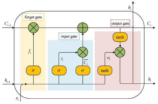
Figure 3.
Internal structure diagram of LSTM.
At time t, the inputs to the LSTM unit are the data, , at this moment; the output, , from the previous moment; and the cell state, , from the previous moment. Meanwhile, at time t, the output, , of this neuron and the cell state, , will also be passed to the next neuron. The specific formulas of LSTM at time t are as follows:
where is the sigmoid activation function, which is used to convert the input to the interval [0, 1]; , , and are the weight values of the forget gate, input gate, and output gate connecting the input and hidden layer neurons, respectively; is the weight value of the cell state; , , , and are bias values; and the tanh activation function converts the input to the interval [−1, 1].
3.3.2. Improved LSTM Power Load Forecasting Model Considering Extreme Weather
Under extreme weather conditions, the uncertainty of power load sequences increases, making load forecasting more difficult. The prediction accuracy of LSTM-based load forecasting models needs to be further improved. To enhance the model’s ability to represent and learn the correlation between front and rear nodes of the load sequence, as well as to reduce computational costs, this paper constructs a dual-layer LSTM load forecasting model in terms of network hierarchy.
In addition, since the LSTM model has many parameters, improper parameter selection will affect the model’s performance to a certain extent. Therefore, the improved particle swarm optimization algorithm based on golden sine (GDPSO) proposed in Section 2 is combined with the LSTM algorithm. Its specific optimization process is similar to that of the GDPSO-SVM model, and the objective function adopts the MAE value of the LSTM prediction model. This can further overcome the blindness in model parameter selection, save computing resources, and improve prediction accuracy.
3.4. Load-Integrated Forecasting Model Considering Extreme Weather
To avoid the shortcomings of a single load forecasting model, ensemble learning algorithms can improve prediction accuracy by combining multiple models for prediction. Therefore, a load-integrated forecasting model is proposed based on a clustering algorithm to realize accurate prediction of power load under extreme weather.
First, preprocess the load and meteorological data. Due to the complex and diverse influencing factors of load under extreme weather conditions, on the basis of load feature extraction, correlation coefficients are used for feature selection. Secondly, the improved SVM algorithm and improved multi-layer LSTM algorithm are used to construct the optimal combination forecasting model. Then, based on the improved power load clustering algorithm, the optimal combination forecasting model is established for various typical loads, thereby constructing a load-integrated forecasting model considering extreme weather. Finally, the predicted values of various typical loads are aggregated to obtain the global load forecasting result to realize load-integrated forecasting considering extreme weather and obtain the changing trend of load characteristics comprehensively considering factors such as extreme weather. The load-integrated forecasting model involves the following key steps:
- The dataset is partitioned into three subsets: training set, validation set, and test set, followed by feature selection. The true values of the validation set are denoted as .
- After initializing the model hyperparameters, the improved support vector machine (SVM) algorithm and the Long Short-Term Memory (LSTM) algorithm are trained on the training set, resulting in trained models and , respectively.
- Based on its performance on the validation set, the GDPSO optimization algorithm proposed in Section 2 is employed to adjust the hyperparameters of each model. This process continues until the maximum number of iterations is reached, yielding the optimal hyperparameter configuration. The predicted values of the improved SVM and LSTM algorithms on the validation set are denoted as and .
- The forecasting errors of the two models are calculated by comparing their predicted values with the true values on the validation set.
- The difference in errors between the two algorithms is computed.
- If the difference is below a predefined threshold, , the two models are combined.
Otherwise, the model with the smaller error is selected.
The final integrated load forecasting result is generated based on the test set.
The specific implementation diagram of the load-integrated forecasting strategy is shown in Figure 4.
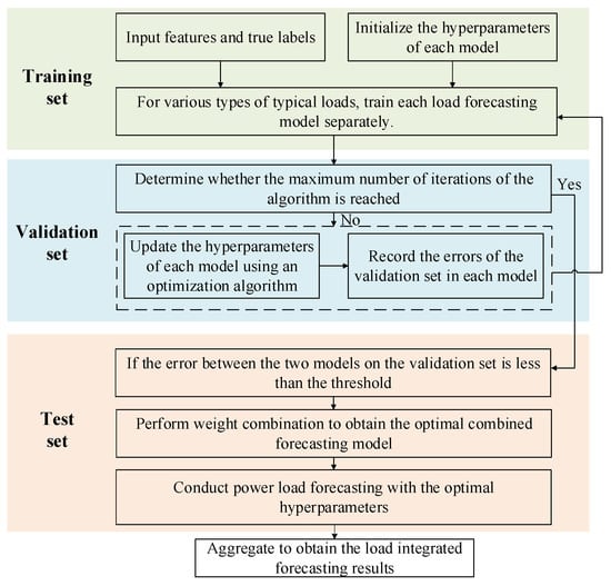
Figure 4.
Schematic diagram of the specific implementation of load forecasting.
3.5. Model Evaluation Indicators
To assess the effectiveness of the load-integrated forecasting model proposed in this paper, three indicators, MAE, RMSE, and , are selected to evaluate the model’s performance. Of these, MAE mainly focuses on the average of the absolute errors of all samples; RMSE mainly focuses on the absolute errors of all samples; and mainly focuses on the overall fitting effect. The specific formulas are as follows:
where is the number of predicted samples; is the actual value of the load; is the predicted value of the load; and is the average value of the load.
The smaller the indicator values of MAE and RMSE, the higher the prediction accuracy of the model; the value range of is [0, 1], and the larger the indicator value, the higher the prediction accuracy of the model.
4. Electric Power and Energy Balance Risk Assessment of New Power System Considering Extreme Weather
With the increase in the penetration rate of new energy and the intensification of climate change, the output of new energy is significantly affected by extreme weather. At the same time, power load fluctuations have further intensified, leading to increased uncertainty in the new power system. The resulting risk of system supply–demand balance may pose threats to its safe and stable operation. In view of this, it is necessary to conduct in-depth research on the balance risk assessment of new power systems considering extreme weather, analyzing and evaluating the risk indicators of power and electricity balance, so as to provide guidance for new power systems to cope with extreme weather.
This section constructs a time-series production simulation model for new power systems considering extreme weather, simulates the production and operation of the system, and conducts a quantitative assessment.
4.1. Time-Series Production Simulation Process Considering Extreme Weather
In the time-series production simulation model considering extreme weather, first, based on the available various types of system data, the boundary conditions for production simulation calculations are determined, including parameters of various units, principles of unit maintenance plans, etc. Then, extreme weather scenarios such as high and low temperatures are set within the research period. During extreme weather periods, adjustments are made to the output of new energy, and random sampling is performed on the upper limit curve of the new energy output to simulate its uncertainty. Meanwhile, on the basis of the original load curve, corresponding power load characteristic curves are generated during extreme weather periods using the load prediction model that takes extreme weather into account. Next, unit maintenance plans are formulated to determine the annual time-series component status of the system. The start–stop status of each unit is calculated through the unit commitment model, and the optimal new energy consumption and system operation cost are obtained based on intraday economic dispatch. Finally, a comprehensive analysis is conducted on the balance risk assessment results of the new power system considering extreme weather.
The specific implementation process of the time-series production simulation considering extreme weather is shown in Figure 5.
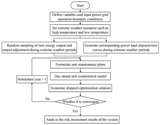
Figure 5.
Flow chart of time-series production simulation considering extreme weather.
- (1)
- Formulation of unit maintenance plans: A reasonable unit maintenance plan is formulated based on the equal reserve method. After arranging the units in a certain order, maintenance of each unit is scheduled in turn during the period of the minimum load.
- (2)
- Solution of unit commitment model: Based on the operation constraints of each unit, a system unit commitment model is established with the goal of minimizing operation costs, start–stop costs, new energy curtailment penalties, load shedding costs, etc., to determine the time-series start–stop status of each unit.
- (3)
- Optimization solution of economic dispatch: On the premise that the day-ahead unit commitment is determined, intraday economic optimization dispatch is carried out. Under the premise of meeting the constraints, the operation cost, curtailment penalty, and load shedding cost are minimized, and a commercial solver is used to determine the output of each unit.
4.2. Generation of Load Curves
This section mainly considers the changes in load levels during extreme weather periods, such as high and low temperatures. The optimal combination forecasting model proposed in Section 3 of this paper, which integrates an improved SVM algorithm and an improved LSTM algorithm, is adopted to generate corresponding power load characteristic curves for extreme weather periods and revise the corresponding periods of the original time-series load curves.
Based on the original load curves, according to the setting of extreme weather scenarios, the influencing factor characteristics of extreme weather periods and the future characteristics of the points to be predicted are taken as inputs. In a single model run, the load prediction model is called to generate hourly corresponding power load characteristic curves for extreme weather periods, such as high and low temperatures, and revise the corresponding periods of the original time-series load curves. These revised curves serve as the load curves for system production simulation. If the original temperature in a certain period of the set extreme weather scenario is already an extreme high or low temperature, the load curve of that period will not be revised. Figure 6 shows the solution process for generating load curves considering extreme weather in the time-series production simulation.
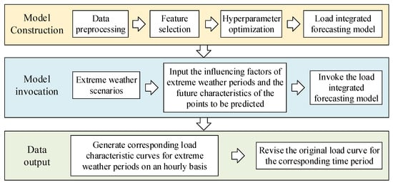
Figure 6.
Schematic diagram of the solution for load curve generation.
4.3. Model Solution and Evaluation Indicators
Based on MATLAB programming, YALMIP + Gurobi is used to optimize and solve the model, and the corresponding solution results and evaluation indicators are output to designated files. Through this, the time-series production simulation results of the power system considering extreme weather are obtained, and then, a comprehensive analysis of the system’s power and electricity balance risks is carried out.
In each simulation year, reliability indicators of the system are calculated. The specific indicators are as follows:
- (1)
- LOLP
- (2)
- EENS
- (3)
- LOLE
- (4)
- MOP
- (5)
- New Energy Consumption Rate
5. Results
The power load curve data of all users in a certain region throughout the year are selected as the research object. The time resolution of the load data is 1 h, and each user’s daily load curve has 24 data points.
Extreme weather conditions in this region are defined as days when the daily minimum temperature is less than or equal to −10 °C or the daily maximum temperature is greater than or equal to 35 °C.
The original load data are subjected to data cleaning and standardization processing so that subsequent analyses are not affected by the scale of users’ electricity consumption. Load curves with missing values reaching 5% or more were considered invalid. For data with missing values below 5%, interpolation methods were applied to fill the gaps in the load data. Finally, 4500 valid load curves are obtained.
All tests in this paper were conducted on a desktop computer equipped with an Intel(R) Core(TM) i7-8700 CPU @ 3.20 GHz and 16.0 GB RAM, and all programming was implemented based on MATLAB R2023b.
5.1. Analysis of Power Load Characteristics Under Extreme Weather Conditions
Before performing dimensionality reduction on the load curves, the traditional k-means algorithm and the improved k-means algorithm are used to cluster the power load curves under extreme weather conditions. The silhouette coefficient, DBI, and CHI are employed to evaluate the clustering effect of each algorithm, and the computational efficiency of the algorithms is assessed by comparing their execution times.
5.1.1. Comparative Analysis of Clustering Effects
The number of clusters in the traditional k-means algorithm is artificially specified, while the improved k-means algorithm proposed in this paper can automatically determine the optimal number of clusters. To make the comparison of experimental results more effective, this paper sets up k-means algorithms with different numbers of clusters (k = 4~7) for power load clustering analysis. The experimental results of different clustering algorithms are shown in Figure 7.
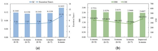
Figure 7.
Comparison of clustering results of different clustering algorithms: (a) SC and execution time; (b) DBI and CHI.
The optimal number of clusters finally obtained by the improved k-means algorithm is four. For the traditional k-means algorithm, in order to achieve the optimal clustering effect, it is necessary to set different numbers of clusters for repeated experiments. From the silhouette coefficient indicator, it can be known that the clustering effect is also relatively good when k = 4.
In Figure 7a, the silhouette coefficient of the improved k-means algorithm is higher, indicating a better clustering effect. However, due to the need for cyclic iteration to find the optimal value, its time consumption has increased.
In Figure 7b, the improved k-means algorithm has the smallest DBI index and the largest CHI index, which further indicates that the improved algorithm has a better clustering effect.
5.1.2. Comparative Analysis of Dimensionality Reduction Effects
Based on the optimal number of clusters being four, the dimensionality reduction effects of the KPCA algorithm and the PCA algorithm in this paper are compared. The relationship between the dimensionality of reduction and the SC index is shown in Figure 8.
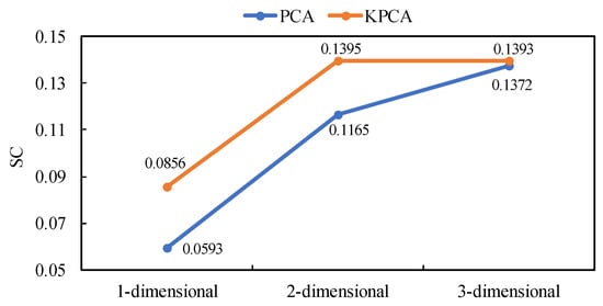
Figure 8.
Relationship between dimensionality and silhouette coefficient index.
Figure 8 shows that the SC values obtained by the KPCA algorithm are larger and more stable than those obtained by the PCA algorithm, demonstrating a better dimensionality reduction effect.
5.1.3. Analysis of Power Load Clustering Results
The power load curve clustering method proposed in this paper, which is based on the KPCA dimensionality reduction method and the improved k-means algorithm, is used to conduct clustering analysis on the power load curves of each user on typical days under extreme weather and normal weather conditions in the region.
Figure 9 and Figure 10 show the power load clustering results under extreme weather and normal weather conditions, respectively. The figures show that the power load curve clustering method put forward in this paper can obtain typical load clustering curves with higher diversity and representativeness under extreme and normal weather conditions, providing a basis for the analysis of power load characteristics under extreme weather based on multi-dimensional load characteristic indicators.
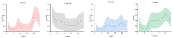
Figure 9.
Clustering results of power load under extreme weather conditions.
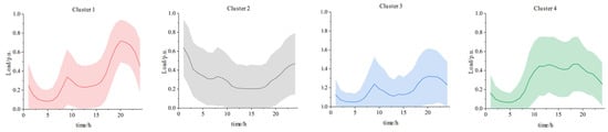
Figure 10.
Clustering results of power load under normal weather conditions.
The comparison results of power load characteristic indicators of each typical cluster under extreme and normal weather conditions are shown in Table 1.

Table 1.
Comparison of typical load characteristic indicators of each cluster.
From the clustering result graphs and the comparison results of load characteristic indicators of each cluster, it can be seen that the power loads of the four clusters present double-peak and double-valley characteristics (Type I), valley-filling characteristics, double-peak and double-valley characteristics (Type II), and continuous or single-peak characteristics. Compared with the clusters under normal weather, the power load of Cluster 1 under extreme weather fluctuates more significantly, with a relatively lower daily load rate and a larger peak–valley difference rate, which may require more peak-shaving capacity to meet the demand during load peaks. The load falling time of Cluster 2 under extreme weather is reduced to 4.1 h, which, to a certain extent, increases the difficulty of “valley-filling” for the power system. The peak–valley time interval of the power load in Cluster 3 under extreme weather still decreases significantly, increasing the difficulty of system regulation. The daily load rate of Cluster 4 under extreme weather obviously decreases, and the load distribution is more unbalanced.
In conclusion, the analysis method for power load characteristics under extreme weather proposed in this section is efficient and accurate. By constructing multi-dimensional load characteristic indicators and improving power load clustering under extreme weather, more diverse and representative typical electricity consumption patterns and their energy consumption under extreme weather on the load side can be obtained, thereby accurately exploring the power load characteristics.
5.2. Analysis of Load-Integrated Forecasting Model Considering Extreme Weather
To verify the effectiveness and generalization ability of this method, the first segment of the test set is selected from the extreme high-temperature weather period, and the second segment is selected from the extreme low-temperature weather period. In addition, two scenarios are set up for the research.
Scenario 1: Without using the load clustering algorithm, the optimal combination forecasting model based on the improved SVM and improved LSTM proposed in Section 3 is compared with other models in terms of forecasting results on the test set.
Scenario 2: Using the load-integrated forecasting strategy, a comparative analysis of forecasting results on the test set is conducted with the optimal combination forecasting model that does not adopt the clustering algorithm.
5.2.1. Feature Selection
Correlation coefficient-based feature selection is adopted to study the correlation characteristics between load and its influencing factors under different weather conditions, and the corresponding results are presented in Table 2.
Table 2.
Absolute value of correlation coefficient.
Table 2 shows that regardless of the weather conditions, the power load has a strong correlation with the moment, real-time temperature, and temperature at adjacent times. During extreme weather periods, the load is more affected by changes in real-time temperature, and the correlation coefficient between the load and real-time temperature is significantly higher. In addition, the correlation coefficient between the load and the weekday/weekend feature is relatively low. Therefore, this feature can be removed in subsequent model training to improve the computational efficiency of the model.
5.2.2. Analysis of Results for Scenario 1
The optimal combination forecasting model based on the improved SVM algorithm and improved LSTM algorithm proposed in this paper is used to predict the total load under extreme weather. Its prediction performance is compared with other prediction models such as the BP neural network model, the traditional SVM model, the traditional LSTM model, and the LSTM-SVM combined prediction model.
- Extreme high-temperature weather
The prediction results of various models under extreme high temperatures are shown in Figure 11. It can be seen from the figure that, in terms of the overall trend, all models can predict the changing trend of load characteristics to a certain extent. However, when the power load has strong volatility and uncertainty under extreme high-temperature weather, the traditional load prediction models have large errors due to their difficulty in capturing the changes in load characteristics. Compared with other single prediction models and combined prediction models, the improved LSTM-SVM optimal combination forecasting model has a higher degree of agreement with the load data under extreme high-temperature weather and thus has certain advantages in load prediction considering extreme high-temperature weather.
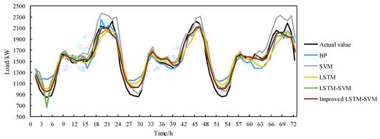
Figure 11.
Comparison of prediction results with various models under extreme high temperatures in Scenario 1.
Figure 12 shows the evaluation indicators of various models under extreme high temperatures.
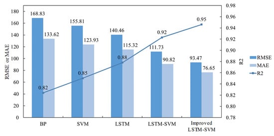
Figure 12.
Comparison of prediction errors of various models under extreme high temperatures in Scenario 1.
It can be seen that, compared with the BP, SVM, LSTM, and LSTM-SVM models, the improved LSTM-SVM optimal combination forecasting model proposed in this paper has its increased by 14.81%, 11.28%, 7.73%, and 2.51%, respectively; its RMSE decreased by 44.64%, 40.01%, 33.45%, and 16.35%, respectively; and its MAE decreased by 42.63%, 38.15%, 33.53%, and 15.60%, respectively. This model has a higher degree of agreement with the load data under extreme high-temperature weather and thus has certain advantages in load prediction considering extreme high-temperature weather.
- Extreme low-temperature weather
The prediction results under extreme low temperatures and the evaluation indicators of these prediction results are presented in Figure 13 and Figure 14, respectively. The error of the optimal combination forecasting model is relatively low.
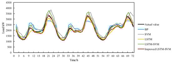
Figure 13.
Comparison of prediction results with various models under extreme low temperatures in Scenario 1.
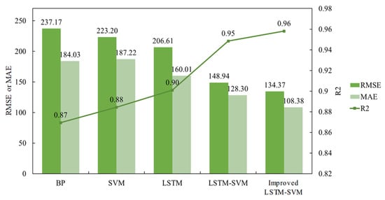
Figure 14.
Comparison of prediction errors of various models under extreme low temperatures in Scenario 1.
This indicates that the proposed optimal combination forecasting model has relatively few errors. This is because the paper uses the GDPSO algorithm for hyperparameter optimization, thereby overcoming the blindness in parameter selection. Moreover, the optimal combination forecasting model can leverage the advantages of each individual model, effectively capture the temporal characteristics of load changes under extreme weather conditions, improve the accuracy of load prediction in extreme weather situations, and possess a certain degree of generalization ability.
5.2.3. Analysis of Results for Scenario 2
To further explore the effectiveness of the proposed load-integrated forecasting model considering extreme weather, the improved clustering method proposed in Section 2 is used to conduct cluster analysis on power loads, with the number of clusters set to four. Then, for each type of typical load under extreme weather, the proposed improved LSTM-SVM optimal combination forecasting model is established to determine the optimal hyperparameters and the corresponding optimal combination forecasting model. After that, the predicted values of various typical loads are aggregated to construct a load-integrated forecasting model, and finally, the global load forecasting results under extreme weather are obtained. These results are compared and analyzed with the forecasting results of the optimal combination forecasting model without using the clustering algorithm on the test set.
- Extreme high-temperature weather
The forecasting results are shown in Figure 15. It can be seen from the figure that when the power load has strong volatility under extreme high-temperature weather, compared with the improved LSTM-SVM optimal combination forecasting model without using the clustering algorithm, the load-integrated forecasting model has a better fitting effect on the load curve under extreme high temperatures.
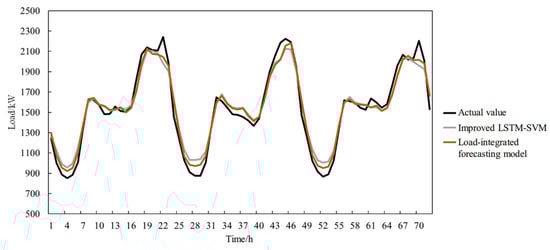
Figure 15.
Comparison of prediction results with various models under extreme high temperatures in Scenario 2.
Figure 16 shows the evaluation indicators of each cluster, the aggregated load-integrated forecasting results, and the forecasting results of the improved LSTM-SVM optimal combination forecasting model without using the clustering algorithm.
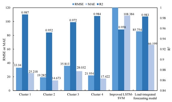
Figure 16.
Comparison of prediction errors of various models under extreme high temperatures in Scenario 2.
The prediction evaluation indicators of most clusters have been significantly improved after load clustering. Overall, the proposed load-integrated forecasting model under extreme high temperatures is superior to the improved LSTM-SVM optimal combination forecasting model. Its is closer to 1, indicating a better overall fitting effect, and both the RMSE and MAE values have been reduced to a large extent, indicating that the load-integrated forecasting model has fewer prediction errors and better prediction performance under extreme high temperatures.
- Extreme low-temperature weather
The prediction results are shown in Figure 17. Figure 18 presents the evaluation indicators of each typical cluster, the aggregated load-integrated forecasting results, and the prediction results of the improved LSTM-SVM optimal combination forecasting model without using the clustering algorithm under extreme low-temperature conditions.
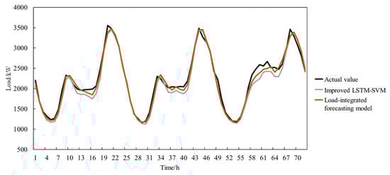
Figure 17.
Comparison of prediction results with various models under extreme low temperatures in Scenario 2.
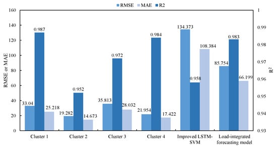
Figure 18.
Comparison of prediction errors of various models under extreme low temperatures in Scenario 2.
Through comparative analysis, it can be known that most of the prediction error indicators of each cluster have also been appropriately improved. The load-integrated forecasting model proposed in this paper under extreme low temperatures has higher prediction accuracy compared with the improved LSTM-SVM optimal combination forecasting model.
In summary, the load-integrated forecasting model considering extreme weather proposed in this paper can integrate the advantages of various models and further reduce the prediction errors caused by load fluctuations under high-temperature and low-temperature extreme weather conditions, and it has good prediction accuracy and generalization abilities. It can realize the accurate prediction of power load under extreme weather.
5.3. Analysis of Time-Series Production Simulation Model Considering Extreme Weather
This paper adopts the improved IEEE RTS79 test system to quantitatively analyze the power and electricity balance risks of the new power system considering extreme weather. The source and load conditions of the system have been adjusted based on the actual load data and new energy output data of a certain region. The topological structure of the system is shown in Figure 19. The system has a total of 24 nodes, 10 conventional thermal power units, and 38 transmission lines. To simulate the new energy output, three wind farms and three photovoltaic power stations are added to this example, and energy storage systems are configured at the nodes of the new energy stations. Some of the technical parameters of the units in the improved IEEE RTS79 test system are listed in Table 3.
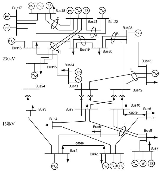
Figure 19.
Topology diagram of the improved IEEE RTS79 test system.
Table 3.
Technical parameters of units in the improved IEEE RTS79 test system.
To comprehensively analyze the impact of extreme weather on the power and electricity balance risks of the new power system, three extreme weather scenarios are set in this example analysis, which are as follows:
Scenario 1: Basic scenario; that is, no additional extreme weather conditions are set.
Scenario 2: The duration of extreme high temperature weather is set to one month (July), and the corresponding load characteristic curve during the extreme high temperature period is generated. Considering the extremely hot and windless conditions, the wind power output limit during the extreme high-temperature period is reduced to 20% of the original output in the same period.
Scenario 3: The duration of extreme low temperature weather is set to one month (January), and the corresponding load characteristic curve during the extreme low temperature period is generated. Considering the extremely cold and sunless conditions, the photovoltaic output limit during the extreme low temperature period is reduced to 20% of the original output in the same period.
5.3.1. Analysis of Load Characteristics Considering Extreme Weather
- Extreme High-Temperature Weather
Typical days are selected for extreme high-temperature weather and normal weather to conduct a comparative analysis of power load characteristics. Figure 20 presents the typical daily load curves.
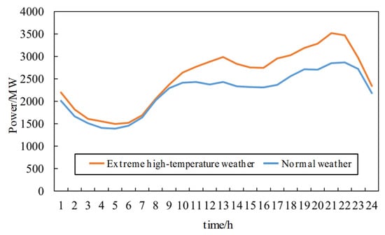
Figure 20.
Typical daily load curves for extreme high-temperature weather and normal weather.
The typical daily power loads in both extreme high-temperature weather and normal weather show a certain “double-peak and double-valley” characteristic, and the power load level during the evening peak is higher than that during the morning peak. The typical load characteristic indicators are shown in Table 4.
Table 4.
Typical load characteristic indicators.
Through load characteristic analysis, it is found that compared with normal weather, both the maximum and minimum loads on typical days in extreme high-temperature weather have significantly increased, with the average load rising by approximately 14.50%. The daily load rate in extreme high-temperature conditions has decreased, indicating that the distribution of power loads is more uneven. Additionally, the daily peak–valley difference rate under extreme high temperatures has increased, which means the power system needs greater peak-shaving capacity to satisfy the load demand in extreme high temperatures, and the difficulty of system regulation has increased.
- Extreme Low-Temperature Weather
Typical days are selected for extreme low-temperature weather and normal weather to conduct a comparative analysis of power load characteristics. The typical daily load curves are shown in Figure 21.
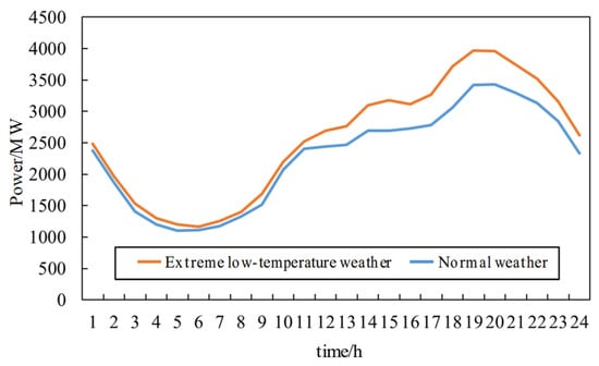
Figure 21.
Typical daily load curves for extreme low-temperature weather and normal weather.
The typical daily power loads in both extreme low-temperature weather and normal weather show an evening peak characteristic. In addition, as shown in Table 5, compared with normal weather, the average load on a typical day in extreme low-temperature weather increases by approximately 12.10%, the load rate decreases slightly, and the peak–valley difference rate rises. A lower load rate in extreme low temperatures will reduce the economy of electricity consumption, while a higher peak–valley difference rate indicates that the load has greater volatility and uncertainty. Therefore, more flexible adjustment measures need to be taken to ensure the safe and stable operation of the system in extreme low-temperature weather.
Table 5.
Comparison of typical load characteristic indicators.
Thus, during extreme weather, the average load of the system increases, the peak–valley difference rate of the load rises, and the load rate decreases. This indicates that the load volatility under extreme weather is enhanced, the load distribution is more uneven, and the system faces the risk of supply–demand balance. A certain peak-shaving capacity and flexible adjustment measures are required to meet the power load demand under extreme weather.
5.3.2. Risk Assessment Results Considering Extreme Weather
By setting corresponding boundary conditions based on the three scenarios, a time-series production simulation model considering extreme weather based on the Monte Carlo method is constructed to simulate the production and operation of the system. This allows for an analysis of the power and electricity balance risk results of the new power system under extreme weather, which mainly include the annual operation results and the production simulation results of typical days under extreme weather.
- Analysis of Annual Operation Results
The annual risk assessment results of the system are shown in Table 6.
Table 6.
The annual risk assessment results of the system.
In the table, , , , and represent the power generation of thermal power, wind power, photovoltaic, and new energy units, respectively; , , and represent the utilization rates of wind power, photovoltaic, and new energy units, respectively.
According to the system’s annual risk assessment indicators under different scenarios, compared with the basic scenario (Scenario 1), due to the decrease in wind turbine output during the extreme high-temperature period in Scenario 2, the annual power generation of wind power units in the system has slightly decreased. Meanwhile, the annual power generation of thermal power and photovoltaic units in the system has increased, thus making up for the shortage of wind power output, alleviating the pressure of ensuring power supply caused by the increase in power load under extreme high-temperature conditions.
In addition, due to the significant decrease in the photovoltaic unit output during the extreme low-temperature period in Scenario 3, the annual power generation of photovoltaic units in the system has decreased, and the utilization rate of new energy has also significantly decreased. Meanwhile, the annual power generation of thermal power and wind power units in the system has increased to a certain extent. Due to the significant decrease in photovoltaic output coupled with the increase in load demand under extreme low-temperature conditions, the system’s loss of load probability reaches 1.51%, the energy shortage reaches 60,971.39 MWh/year, and the expected power shortage time reaches 5.5 days/year. Compared with Scenario 1, the reliability level is significantly reduced, and the risk of supply–demand imbalance increases.
- Analysis of Typical Daily Operation Results
Based on the above analysis, typical days are selected during the extreme high-temperature period of Scenario 2 and the extreme low-temperature period of Scenario 3 to conduct an analysis of the system’s supply–demand balance risks, as shown in Figure 22 and Figure 23, respectively. These figures include the power load demand under extreme weather and the time-series output of each unit in the system.
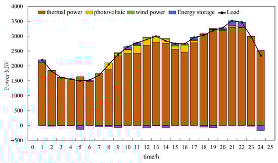
Figure 22.
Balance results for a typical day in Scenario 2.
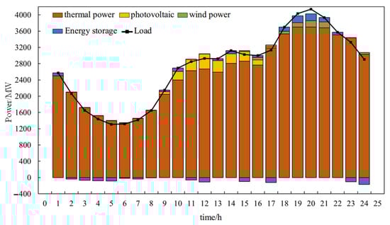
Figure 23.
Balance results for a typical day in Scenario 3.
Figure 22 shows the balance results for a typical day during the extreme high-temperature period (Scenario 2). The maximum load demand of the system on that day is 3518 MW, which is supplied by thermal power, photovoltaic power, wind power, and energy storage. As the temperature gradually rises during the day, the load demand continues to increase, requiring thermal power units to increase their output through ramping and start–stop operations. Photovoltaic output increases at noon, while wind power output remains relatively low due to the impact of extreme weather. Therefore, photovoltaic units mainly cover the peak load demand at noon, which alleviates the ramping pressure on thermal power. In order to avoid curtailment of new energy, energy storage devices store the excess electricity at this time. The power load reaches another evening peak between 19:00 and 22:00. During this period, photovoltaic output is almost zero. Moreover, due to the constraints of extreme high-temperature weather, wind turbine output is limited, resulting in an 83% drop in new energy output during this period. The combined output of thermal power and new energy is insufficient to meet the evening peak load demand, leading to a risk of load loss. However, energy storage devices quickly release the stored electricity, effectively mitigating the high fluctuations in power load demand and new energy output caused by extreme high temperatures.
Figure 23 shows the balance results for a typical day during the extreme low-temperature period (Scenario 3). The maximum load demand of the system is 4139 MW. Compared with Scenario 2, the load level in Scenario 3 is high, with a larger peak–valley difference and stronger volatility in the power load. The composition of units supplying the load is the same as that on a typical day of extreme high temperatures. The power generation of wind power units on the typical day of extreme low temperatures increases slightly overall. The wind power output during the evening peak period of load is about twice that of the same period on the typical day of extreme high temperatures. Due to the constraints of the system’s source and load conditions, the absorption rate of photovoltaic units is relatively high, and the photovoltaic output on the typical day of extreme low temperatures is relatively large during the noon period. During the low load period at night and when the new energy power generation is large at noon, energy storage maintains the system’s power and electricity balance by effectively storing electricity and discharging it quickly during peak load periods. The average load on the typical day of extreme low temperatures increases, the peak–valley difference expands, and the power load level during the evening peak period rises. The combined output of thermal power units, new energy, and energy storage discharge is still insufficient to meet the load demand during the evening peak. The insufficient adequacy of the system leads to a load loss from 19:00 to 20:00 on this typical day, with an energy shortage of 165 MW. Therefore, more flexible adjustment measures need to be taken to meet the power and electricity balance demand of the system under extreme weather.
In summary, when the load demand under extreme weather is high and the volatility of new energy is large, the system will face the risk of supply–demand imbalance. The power and electricity imbalance of the example system is more serious in the extreme low-temperature scenario. Therefore, more flexible adjustment measures need to be taken, such as flexible transformation of thermal power units, formulation of reasonable demand response strategies, and increasing the proportion of flexible resources, such as energy storage, so as to further enhance the resilience and secure operation of the new power system in the face of extreme weather.
6. Conclusions
With the advancement of global climate change and the construction of new power systems, the increasing frequency of extreme weather, coupled with the diversification and complexity of power loads, has posed severe challenges to the safe and stable operation of power systems and the balance between power supply and demand. Therefore, this paper conducts research on the analysis of power system load characteristics and the risk assessment of power and electricity balance under extreme weather.
Firstly, this paper proposes an improved power load clustering method based on the KPCA nonlinear dimensionality reduction method and the improved k-means algorithm. Case analysis shows that compared with traditional methods, the proposed method in this paper is highly efficient and accurate.
Secondly, the improved PSO algorithm proposed in Section 2 is used to optimize the hyperparameters of the prediction model. The improved SVM algorithm and the improved LSTM algorithm are adopted to construct the optimal combination forecasting model. Based on the improved power load clustering algorithm, a load-integrated forecasting model considering extreme weather is constructed. Through case verification, it can be seen that this model has better load prediction performance during extreme weather periods, enabling more accurate load prediction under extreme weather and providing data support for the subsequent system balance risk assessment considering extreme weather.
Finally, based on the load-integrated forecasting model, a time-series production simulation model for new power systems considering extreme weather is constructed, and a comprehensive comparative analysis of the power and electricity balance risks of new power systems under extreme weather is conducted. The results show that the example system exhibits different supply–demand balance risk issues in extreme scenarios. When the load demand under extreme weather is high and the volatility of new energy is large, the system will face the risk of supply–demand imbalance. More flexible adjustment measures should be taken to further enhance the resilience and secure operation of the new power system in the face of extreme weather.
In the future, in the research on power load characteristic analysis methods under extreme weather, the integration of other intelligent optimization algorithms, deep learning techniques, and data augmentation methods can further enhance the accuracy of such analysis. Subsequent studies on load forecasting methods considering extreme weather could incorporate additional factors in feature extraction—such as humidity, air pressure, and electricity prices—while leveraging various machine learning algorithms for feature selection and processing. Moreover, combining the model proposed in this paper with other more efficient approaches in load forecasting would help improve both its accuracy and generalization capabilities under extreme weather conditions. In terms of risk assessment for system balance under extreme weather, as the system scale expands, the computational efficiency of the method proposed in this paper requires further improvement. Future work may also incorporate multiple flexibility resources, electricity market mechanisms, and various extreme weather scenarios. Such enhancements would effectively improve the efficiency and comprehensiveness of balance risk assessment while ensuring solution accuracy.
Author Contributions
Conceptualization, M.S. and D.C.; methodology, M.S., C.Z., and Y.L.; software, D.C. and S.H.; validation, J.L.; formal analysis, Y.L.; investigation, C.Z.; data curation, M.S. and C.Z.; writing—original draft preparation, C.Z. and Y.L.; writing—review and editing, G.L. and Y.B.; supervision, G.L. and Y.B. All authors have read and agreed to the published version of the manuscript.
Funding
This work is supported by the Research Project of the State Grid Corporation of China (Project No. 2024YF-44).
Data Availability Statement
The original contributions presented in this study are included in the article. Further inquiries can be directed to the corresponding author.
Conflicts of Interest
Author Mingyi Sun, Dai Cui, Shubo Hu, and Jiayi Li are employed by the company State Grid Liaoning Electric Power Supply Co., Ltd. The remaining authors declare that this research was conducted in the absence of any commercial or financial relationships that could be construed as potential conflicts of interest.
References
- Zhong, H.W.; Zhang, G.L.; Cheng, T.; Ye, Y. Analysis and Enlightenment of Extremely Cold Weather Power Outage in Texas, U.S. in 2021. Autom. Electr. Power Syst. 2022, 46, 1–9. [Google Scholar]
- Gao, H.J.; Guo, M.H.; Liu, J.Y.; Liu, J.T.; He, J.S. Power Supply Challenges and Prospects in New Power System from Sichuan Electricity Curtailment Events Caused by High-temperature Drought Weather. Proc. CSEE 2023, 43, 4517–4538. [Google Scholar]
- Chen, B.; Liao, J.L. Technology for Improving Distribution Network Disaster-Prevention Capabilities for Intercurrent Natural Disasters Areas Under Extreme Weather: Review and Prospect. Electr. Power Constr. 2025, 46, 107–121. [Google Scholar]
- Zhao, J.Y.; Fu, Y.J.; Fan, H.G.; Ge, L.; Hu, C.S.; Zhao, H.F. Analysis of Non-invasive Power Grid Load Characteristics Based on Big Data Analytics. Autom. Technol. Appl. 2025, 44, 38–42. [Google Scholar]
- Ye, Q.; Chen, W.X.; Jiang, Z.Y.; Cai, Y.Q.; Xiao, Y.Q.; Jing, R.; Zhao, Y.R. Multi-city Industry-level Load Profiling and Cooling Load Measurement Considering Summer Hotwaves. Global Energy Interconnect. 2024, 7, 25–36. [Google Scholar]
- Wang, Z.; Wu, Q.; Bao, X.H.; Liu, S.H.; Zhang, G.Y.; Wang, K.F.; Zhu, J.B. Analysis on Response Potential of Comprehensive Energy User Demand Based on Quadratic Clustering. Electr. Eng. 2023, 5, 43–47. [Google Scholar]
- Song, J.Y.; He, C.; Li, X.R.; Liu, Z.G.; Tang, J.; Zhong, W. Daily Load Curve Clustering Method Based on Feature Index Dimension Reduction and Entropy Weight Method. Autom. Electr. Power Syst. 2019, 43, 65–72. [Google Scholar]
- Ji, Y.Q.; Yan, Y.B.; He, P.; Liu, X.M.; Li, C.S.; Zhao, C.; Fan, J.L. CNN-LSTM short-term load forecasting based on the K-Medoids clustering and grid method to extract load curve features. Power Syst. Prot. Control 2023, 51, 81–93. [Google Scholar]
- Xu, X.F.; Zhao, Y.; Liu, Z.Z.; Li, L.J.; Lu, Y. Daily Load Characteristic Classification and Feature Set Reconstruction Strategy for Short-term Power Load Forecasting. Power Syst. Technol. 2022, 46, 1548–1556. [Google Scholar]
- Han, F.J.; Pu, T.J.; Li, M.Z.; Taylor, G. Short-term forecasting of individual residential load based on deep learning and K-means clustering. CSEE J. Power Energy Syst. 2021, 7, 261–269. [Google Scholar]
- Lin, S.F.; Li, F.X.; Tian, E.W.; Fu, Y.; Li, D.D. Clustering load profiles for demand response applications. IEEE Trans. Smart Grid 2017, 10, 1599–1607. [Google Scholar] [CrossRef]
- Zhang, C.R. Research on Short-Term Power Load Forecasting and Load Curve Clustering Based on Machine Learning. Master’s Thesis, Zhejiang University, Hangzhou, China, 2021. [Google Scholar]
- Fan, Y.H.; Jiang, T.Y.; Huang, Q.F.; Ju, P. Portrait-based Assessment on Demand Response Potential of Industrial Parks. Autom. Electr. Power Syst. 2024, 48, 41–49. [Google Scholar]
- Qin, R.S.; Kuang, H.; He, X.; Duan, R.M. Cluster Analysis of Actual Daily Load Curve Based on Improved PSO-Kmeans Algorithm. Electr. Eng. 2022, 11, 1–6. [Google Scholar]
- Xu, S.L.; Xu, J. User Daily Load Classification Method Based on Improved Deep Clustering Under Spark Architecture. Mod. Electr. Power 2025, 42, 411–420. [Google Scholar]
- Stief, A.; Ottewill, J.R.; Baranowski, J.; Orkisz, M. A PCA and two-stage Bayesian sensor fusion approach for diagnosing electrical and mechanical faults in induction motors. IEEE Trans. Ind. Electron. 2019, 66, 9510–9520. [Google Scholar] [CrossRef]
- Chen, Z.F.; Bao, M.; Ge, L.J.; Ma, C.; Jiao, Q.Y. Deep Embedding Clustering Method of Power Load Based on Asymmetric Convolutional Autoencoder with Label Optimization. Electr. Autom. Equip. 2024, 44, 69-75+99. [Google Scholar]
- Selvi, M.V.; Mishra, S. Investigation of performance of electric load power forecasting in multiple time horizons with new architecture realized in multivariate linear regression and feed-forward neural network techniques. IEEE Trans. Ind. Appl. 2020, 56, 5603–5612. [Google Scholar] [CrossRef]
- Smyl, S. A hybrid method of exponential smoothing and recurrent neural networks for time series forecasting. Int. J. Forecast. 2020, 36, 75–85. [Google Scholar] [CrossRef]
- Li, G.Q.; Liu, Z.; Jin, G.B.; Quan, R. Ultra Short-Term Power Load Forecasting Based on Randomly Distributive Embedded Framework and BP Neural Network. Power Syst. Technol. 2020, 44, 437–445. [Google Scholar]
- Yang, Y.L.; Che, J.X.; Deng, C.Z.; Li, L. Sequential grid approach based support vector regression for short-term electric load forecasting. Appl. Energy 2019, 238, 1010–1021. [Google Scholar] [CrossRef]
- Kong, X.Y.; Li, C.; Zheng, F.; Wang, C.S. Improved deep belief network for short-term load forecasting considering demand-side management. IEEE Trans. Power Syst. 2019, 35, 1531–1538. [Google Scholar] [CrossRef]
- Gunawan, J.; Huang, C.Y. An extensible framework for short-term holiday load forecasting combining dynamic time warping and LSTM network. IEEE Access 2021, 9, 106885–106894. [Google Scholar] [CrossRef]
- Feng, Y.; Song, Y.B.; Jin, S.; Feng, J.H.; Shi, X.C.; Yu, Y.J.; Huang, X.C. Improved Deep Learning Short-Term Load Based on Random Forest Algorithm and Rough Set Theory. Power Gener. Technol. 2023, 44, 889–895. [Google Scholar]
- Huang, F.H.; Zhao, H.L.; Yi, P.Y.; Li, P.D.; Peng, J. An Improved Power Load Forecasting Method Based on Transformer. Mod. Electr. Power 2023, 40, 50–58. [Google Scholar]
- Liu, J.; Cong, L.M.; Xia, Y.Y.; Pan, G.Y.; Zhao, H.C.; Han, Z.Y. Short-Term Power Load Prediction Based on DBO-VMD and IWOA-BILSTM Neural Network Combination Model. Power Syst. Prot. Control 2024, 52, 123–133. [Google Scholar]
- Wang, Y.F.; Cao, Y.H.; Sun, J.W. Short-Term Power Load Forecasting Based on Multi-Strategy Improved Golden Jackal Algorithm-Optimized LSTM. Power Syst. Prot. Control 2024, 52, 95–102. [Google Scholar]
- Sharma, A.; Jain, S.K. A novel two-stage framework for mid-term electric load forecasting. IEEE Trans. Ind. Inf. 2024, 20, 247–255. [Google Scholar] [CrossRef]
- Li, N.; Jiang, T.; Sui, X.; Hu, Y.X. A Multi-Component Short-Term Power Load Combination Forecasting Method on a Time-Frequency Scale. Power Syst. Prot. Control 2024, 52, 47–58. [Google Scholar]
- Fan, J.M.; He, G.L.; Zhong, M.W.; Wang, X.G.; Xu, L.; Ke, Z.W. Short-Term Load Forecasting for Date Mode Equivalent and Multi-Level Parallel Convolution Modules is Considered. Power Syst. Technol. Power Syst. Technol. 2025, 49, 2554–2562. [Google Scholar]
- Shen, H.T.; Li, F.; Shi, L.; Sun, S.B.; Yang, Z.N.; Yang, T. Short-Term Power Load Forecasting Based on Reduction of Meteorological Data Dimensionality and Hybrid Deep Learning. Electr. Power Constr. 2024, 45, 13–21. [Google Scholar]
- Wang, Y.L.; Liu, Z.Q.; Dong, H.R.; Li, D.X.; Chen, X.; Guo, L.; Wang, J.R. Multivariate Load Forecasting of Integrated Energy System Based on CEEMDAN-CSO-LSTM-MTL. Electr. Power Constr. 2025, 46, 72–85. [Google Scholar]
- Meng, H.; Zhang, T.; Wang, J.; Zhang, J.Y.; Li, D.; Shi, G.R. Multi-node Short-term Power Load Forecasting Method Based on Multi-scale Spatiotemporal Graph Convolution Network and Transformer. Power Syst. Technol. 2024, 48, 4297–4311. [Google Scholar]
- Xie, Q. Research on Consumer Load Forecasting Considering Power Consumption Behavior under Special Events. Master’s Thesis, North China Electric Power University, Beijing, China, 2022. [Google Scholar]
- Dai, M.M.; Wang, K.; Li, Q.; Shi, J.F.; Deng, Y.W.; Zhang, R.R.; Liu, R.H.; Sun, G.P. Short-term Load Forecasting Method Based on Weather Classification and Convolutional Neural Network. Power Demand Side Manag. 2023, 25, 93–98. [Google Scholar]
- Feng, J.H.; Shi, X.C.; Zhang, Y.; Hu, T.; Feng, J.; Hong, C.W.; Hong, Y.; Wu, Y.T. Short-Term Load Forecasting Based on Low-Rank Completion Algorithm in Extreme Weather. Distrib. Energy. 2024, 9, 51–59. [Google Scholar]
- Vapnik, V.; Golowich, S.E.; Smola, A. Support vector method for function approximation, regression estimation, and signal processing. Adv. Neural Inf. Process. Syst. 2008, 9, 281–287. [Google Scholar]
- Yao, C.W.; Yang, Z.H.; Bai, H.M.; Wu, Y.Z.; Gong, Z.Q.; Feng, G.L. Ensemble prediction of winter precipitation in China based on Support Vector Machine Method. Chin. J. Geophys. 2024, 67, 3670–3685. [Google Scholar]
- Xu, W.; Jiang, Y.N.; Zhang, X.L.; Li, Y.; Zhang, R.; Fu, G.T. Using long short-term memory networks for river flow prediction. Hydrol. Res. 2020, 51, 1358–1376. [Google Scholar] [CrossRef]


Disclaimer/Publisher’s Note: The statements, opinions and data contained in all publications are solely those of the individual author(s) and contributor(s) and not of MDPI and/or the editor(s). MDPI and/or the editor(s) disclaim responsibility for any injury to people or property resulting from any ideas, methods, instructions or products referred to in the content. |
© 2025 by the authors. Licensee MDPI, Basel, Switzerland. This article is an open access article distributed under the terms and conditions of the Creative Commons Attribution (CC BY) license (https://creativecommons.org/licenses/by/4.0/).