Adapting Gated Axial Attention for Microscopic Hyperspectral Cholangiocarcinoma Image Segmentation

Abstract

Accurate segmentation of medical images is essential for clinical diagnosis and treatment planning. Hyperspectral imaging (HSI), with its rich spectral information, enables improved tissue characterization and structural localization compared with traditional grayscale or RGB imaging. However, the effective modeling of both spatial and spectral dependencies remains a significant challenge, particularly in small-scale medical datasets. In this study, we propose GSA-Net, a 3D segmentation framework that integrates Gated Spectral-Axial Attention (GSA) to capture long-range interband dependencies and enhance spectral feature discrimination. The GSA module incorporates multilayer perceptrons (MLPs) and adaptive LayerScale mechanisms to enable the fine-grained modulation of spectral attention across feature channels. We evaluated GSA-Net on a hyperspectral cholangiocarcinoma (CCA) dataset, achieving an average Intersection over Union (IoU) of 60.64 ± 14.48%, Dice coefficient of 74.44 ± 11.83%, and Hausdorff Distance of 76.82 ± 42.77 px. It outperformed state-of-the-art baselines. Further spectral analysis revealed that informative spectral bands are widely distributed rather than concentrated, and full-spectrum input consistently outperforms aggressive band selection, underscoring the importance of adaptive spectral attention for robust hyperspectral medical image segmentation.

1. Introduction

Medical imaging in clinical settings has two complementary requirements: security and computer-aided diagnosis and therapy (CADT). Security can be addressed using hyperchaotic image encryption in the image layer [1] and intrusion-detection-embedded chaotic encryption in the link layer [2]. Maintaining accuracy during image corruption is a parallel concern, as highlighted by robustness-oriented parsing with boundary-aware high-resolution features and a polar harmonic Fourier moment (PHFM) domain transform [3]. We emphasize the CADT side as primary for patient care; efficient and accurate medical image segmentation is central to medical image analysis and underpins computer-aided diagnosis and therapy. In this context, deep learning has become the de facto paradigm for medical-image segmentation.

The excellent performance of deep learning in ILSVRC12 has proven its capability to recognize complex images and has driven the widespread use of deep convolutional neural networks (CNNs) in computer vision (CV). CNNs have been employed not only for image classification, but also for image segmentation. Segmentation networks, including U-Net [4,5], 3D U-Net [5,6], SegResNet [7], SwinUNETR [8], and DynUNet [9], have been widely applied in different medical imaging tasks, proving that CNNs can capture anatomical and pathological information from medical images.

Recently, there has been a growing interest in transformers [10,11] for image processing, and transformers have become an alternative framework to replace traditional CNN-based methods [12,13,14]. In standard CNNs, a local receptive field exists for each convolutional kernel. Although deeper CNNs can integrate a larger spatial context at deeper layers, they also have difficulty in modeling long-range dependencies. This limitation has been largely alleviated by transformers by virtue of global-context modeling. Transformers were first introduced for natural language processing (NLP) but have recently been extended to image recognition. Studies such as [15] have demonstrated that adopting transformers in U-Net networks can be an efficient way to boost the segmentation performance. In addition to transformer-based designs, recent studies [16] have proposed hybrid detection–contour frameworks that use a deep detector to automatically initialize classical active contours and combine edge-preserving diffusion for robust boundaries, achieving competitive instance segmentation on standard datasets [17].

With the significant development of artificial intelligence, the substantially restricted information in conventional imaging modalities limits the performance of pre-existing deep neural networks. Typical grayscale and RGB images are void of any sense or dimension (spatial as well as color-wise) and hence are inadequate for delineating anatomical structures with identical intensity histograms. In cases where the organs/lesions are characterized by subtle colors, and pixel intensities are closely related to their surrounding tissues, it is very difficult to perform precise segmentation using deep neural networks.

An increasing number of deep learning models [18,19,20,21,22,23] have been applied to hyperspectral image (HSI) segmentation, taking full advantage of the rich spectral information provided by hyperspectral images. HSI is a fusion of spatial and spectral information and is commonly employed for fine-grained classification in remote sensing. In addition to Earth observations, hyperspectral imaging has been utilized in agriculture and medical services. Meanwhile, targeting the medical field, a CNN-based pixel-wise classification technique for head and neck cancer detection from medical hyperspectral datasets was presented in [24]. Despite these benefits, this method does not make full use of the spatial characteristics of hyperspectral images and is not an optimal choice for application to scenes where the spectral difference between classes is small, resulting in poor segmentation accuracy.

To solve this problem, HyperUNet was proposed in [19], in which U-Net was used for hyperspectral segmentation based on spectral-spatial features. However, the structure of the traditional U-Net is unsuitable for capturing the global spatial dependencies of hyperspectral data. To resolve this issue, Zhang et al. [23] presented the SAHIS-Net, which incorporates transformers into hyperspectral image segmentation. However, in general, spectral dimensions are treated as individual input channels for a 2D model and natural spectral correlations are not utilized. This has motivated the exploration of 3D convolutional architectures for hyperspectral segmentation. SpecTr was proposed in [18], which leverages 3D convolution to learn local spatial and spectral characteristics, and applies spectral attention to model global spectral relationships. This method greatly enhances the segmentation performance of medical hyperspectral data.

The feature pyramid network (FPN) architecture [25] fuses high-level semantic features with low-level spatial details through top-down pathways and lateral connections, making it suitable for small target segmentation and compatible with attention-based encoders. Building upon the hierarchical structure of the Swin Transformer [26], we designed GSA-Net by employing 3D depthwise convolutions in the encoder and a 3D FPN in the decoder, where the decoder also integrates a lightweight Spectral Pyramid Fusion (SPF) module for moderate multi-scale spectral refinement. The Gated Spectral-Axial Attention (GSA) module was embedded in the encoder to enhance spectral modeling by capturing the inter-band dependencies along the spectral axis. Owing to the complexities of the 3D model and difficulty of training, we introduced lightweight Multilayer Perceptron (MLP) layers and adaptive scaling coefficients into the GSA module. These modifications improve the gradient flow and stability of training in limited batches.

A key innovation in GSA-Net is the incorporation of the Gated Spectral-Axial Attention (GSA) module, which is embedded in the encoder to enhance spectral dependency modeling across hyperspectral bands. By aggregating the mean spectral features and using axial attention along the spectral dimension, GSA-Net can capture subtle spectral variations among different tissue types, which is critical for hyperspectral medical imaging. Overall, GSA-Net demonstrates that attention-based architectures can be effectively adapted and optimized for hyperspectral imaging tasks, highlighting their practical relevance for fine-grained biomedical segmentation applications.

2. Materials and Methods

The proposed model is shown in Figure 1. The input was a hyperspectral image ($X_{hsi}\in {ℝ}^{S\times H\times W}$). The number of bands in the hyperspectral image is S, height is H, and width is W. The model can be divided into two parts, encoding and decoding.

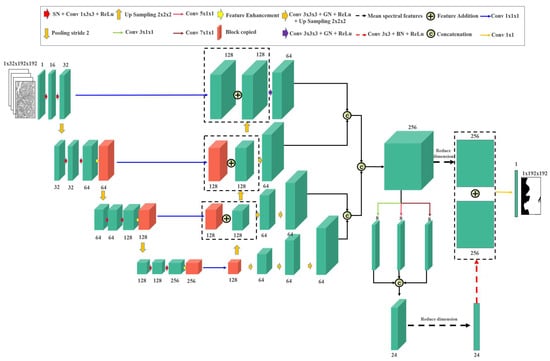
Figure 1. Overview of Gated Spectral-Axial Net (GSA-Net).

2.1. Encoder Block

The encoder consisted of several convolution and transformer blocks. Each convolution block includes spectral normalization and leaky rectified linear unit activation in addition to the convolution operation, which can be represented as:

$$\mathrm{ConvBlock}(X,W,b)=\sigma (Spectral\mathrm{Norm}(\mathrm{Conv}(W\ast X+b)))$$

(1)

where W denotes the weight parameter of the convolution kernel, which can be considered a 3D convolution kernel. SpectralNorm denotes the Spectral Normalization operation. Additionally, b denotes the bias term and $\sigma$ denotes the activation function.

The three-dimensional (3D) convolution model is shown in Figure 1. In the first layer, the hyperspectral input consisted of a single-channel feature map. Through two successive convolutional operations with a kernel size of 1 × 3 × 3 and a stride of 1 × 1 × 1, the feature representation was expanded to 32 channels, enabling the model to extract low-level spatial-spectral features effectively.

From the second layer onward, the network progressively reduced the spatial and spectral resolutions using 3D convolutions with a stride of 2 × 2 × 2, thereby building hierarchical features across scales. Each encoding stage comprises a spectral regularization module, spatial-spectral convolutional blocks, and a transformer-based feature enhancement module. Spectral normalization is performed along the spectral dimension using GroupNorm, standardizing each spectral channel independently. By contrast, conventional 3D normalization (e.g., BatchNorm3D) aggregates statistics across both spatial and spectral dimensions, effectively forcing all spectral channels to share a single distribution. For hyperspectral data, where each band has unique intensity and feature characteristics, this mixing can obscure important spectral differences. By applying normalization per spectral channel, which is conceptually similar to applying standard 2D normalization on each band separately, our approach preserves the intrinsic differences between spectral bands while reducing the spatial distribution variability within each band, thereby stabilizing optimization and improving feature learning. The subsequent transformer module models long-range spectral dependencies and enhances global context representation.

In summary, each layer of the encoder is expressed as follows.

$$E_1=\mathrm{Transformer}(g(X,W_1,b_1,\mathrm{stride}=1))$$

(2)

$$E_1^{down}=\mathrm{ConvBlock}(E_1,W_1^{\mathit{down}},b_1^{\mathit{down}},\mathrm{stride}=2)$$

(3)

$$D_k^{\mathrm{up}}=\mathrm{ConvTransposed}(D_{k+1},W_k^{\mathrm{up}},b_k^{\mathrm{up}};\mathrm{stride}=2),k=1,2,3,\dots$$

(4)

where $E_1$ denotes the first-layer encoded features, such as the red blocks in the first layer of Figure 1. $g(\cdot )$ denotes the features after two convolutional block processes, $E_1^{down}$ denotes the features after downsampling for the first-layer network, $E_{k-1}^{down}$ denotes the features after downsampling for the (k − 1)-th layer network, and $E_k$ denotes the k-th layer encoded features. $W_1$, $b_1$, $W_1^{\mathit{down}}$, $b_1^{\mathit{down}}$, $W_k$ and $b_k$ denote the weight parameters of the convolution kernel of the first-layer network, bias term of the first-layer network, weight parameters of the downsampled convolution kernel of the first-layer network, downsampled bias term of the first-layer network, weight parameters of the convolution kernel of the k-th layer network, and bias term of the k-th layer network, respectively.

2.2. Decoder Block

The decoder follows a top-down path similar to the Feature Pyramid Network (FPN) structure, where feature maps from different encoder stages are gradually upsampled and fused with higher-resolution features through skip connections. This structure enables the model to recover fine spatial details while preserving the semantic context extracted at deeper levels.

To further enhance the cross-scale representation, we employed a Spectral Pyramid Fusion (SPF) module that aggregates multi-resolution information while focusing on spectral patterns. For each decoder level, the feature map is first upsampled by a 3D transposed convolution with a stride of 2 × 2 × 2 and then added element-wise to the corresponding encoder feature map. The fused output is fed into three parallel 3D convolutional branches whose kernels extend only along the spectral axis: 3 × 1 × 1, 5 × 1 × 1, and 7 × 1 × 1. This design allows the network to adaptively model long-range spectral dependencies at multiple receptive fields while keeping the spatial footprint unchanged, leading to richer contextual cues for the subsequent decoding stages.

The overall decoder process can be formulated as follows:

$$D_k^{\mathrm{up}}=\mathrm{ConvTransposed}(D_{k+1},W_k^{\mathrm{up}},b_k^{\mathrm{up}};\mathrm{stride}=2),k=1,2,3,\dots$$

(5)

$$A_k=D_k^{\mathrm{up}}\hspace{0.33em}\oplus \hspace{0.33em}{E}_k^{down},k=1,2,3,\dots$$

(6)

$$U_k=\mathrm{Conv}3\mathrm{D}(\mathrm{Upsample}\left(A_k;s=2^{k-1}\right),W_k^u,b_k^u),k=1,2,3,\dots$$

(7)

$$S\hspace{0.33em}=\hspace{0.33em}{U}_1\hspace{0.33em}\Vert \hspace{0.33em}{U}_2\hspace{0.33em}\Vert \hspace{0.33em}\dots \Vert \hspace{0.33em}{U}_k,k=1,2,3,\dots$$

(8)

$$B_p={\mathrm{Conv}}^{p\times 1\times 1}(S,W_p,b_p),\hspace{0.33em}\hspace{0.33em}\hspace{0.33em}p\in \{3,5,7\}$$

(9)

$$F_{\mathrm{spf}}=B_3\hspace{0.33em}\Vert \hspace{0.33em}{B}_5\hspace{0.33em}\Vert \hspace{0.33em}\hspace{0.33em}{B}_7$$

(10)

$$M=\hspace{0.33em}{\mathrm{Mean}}_s(S)\oplus \mathrm{ReLU}\left(\mathrm{Norm}\right(\mathrm{Conv}2\mathrm{D}({\mathrm{Mean}}_s(F_{\mathrm{spf}}),W_{\mathrm{spf}},b_{\mathrm{spf}})))$$

(11)

$$\widehat{Y}=\sigma (\mathrm{Conv}2\mathrm{D}(M,W_{\mathrm{out}},b_{\mathrm{out}}))$$

(12)

where $D_{k+1}$ denotes the underlying decoder features, $E_k^{down}$ denotes the features after downsampling of the k-th layer network, $\mathrm{ConvTransposed}(\cdot )$ denotes the upsampling operation, $D_k^{up}$ denotes the features after upsampling of the k-th layer network, and $A_k$ denotes the element-wise sum of the decoder and skip features. $\mathrm{Upsample}\left(\cdot ;s=2^{k-1}\right)$ enlarges the spatial–spectral size such that all levels have the same resolution as the first decoder level. $U_k$ is the output of a 3D convolution applied to the upsampled characteristic $A_k$. In addition, $\Vert$ denotes a concatenation operation. $B_p$ is a branch feature of the Spectral-Pyramid-Fusion (SPF) module with spectral kernel size $p\in \{3,5,7\}$. $M$ is the feature obtained by first averaging along the spectral dimension (${\mathrm{Mean}}_s$), then applying a 2-D convolution, normalization, and ReLU. $\widehat{Y}$ denotes the final predicted segmentation map.

2.3. Transformer Block

Each convolutional kernel in the traditional CNN model can only focus on the local features of the image, whereas the stacked convolutional neural network is still unable to grasp the global context, even though it focuses on more image information in the last few layers of the network. To better extract the global features of hyperspectral images, we introduced a transformer module [27,28,29,30] in the encoding part.

Common transformer-based architectures for visual processing include the Vision Transformer (ViT), Pyramid Vision Transformer (PVT), and the Axial Transformer. ViT represents the canonical global self-attention mechanism introduced in the Vision Transformer, which effectively captures long-range dependencies, but typically requires large-scale datasets and incurs high computational costs. This architecture is widely used for sequence modeling but is less efficient for dense visual tasks. PVT introduces spatially reduced attention along with a pyramid structure to enhance scalability, making it more suitable for dense prediction tasks, such as image segmentation. This approach was adopted in the fault diagnosis of HVAC systems using thermal images and demonstrated improved spatial scalability and computational efficiency [29]. The Axial Transformer, originally proposed for medical image segmentation, factorizes 2D attention into separate height- and width-wise branches. This decomposition improves directional modeling efficiency and reduces the number of parameters.

2.3.1. Gated Axial Attention

We adopted the Gated Axial Attention (GAA) originally proposed for RGB medical images in a Medical Transformer [31]. The encoder feature map is routed to two parallel axial-attention branches, Gated Height-Axial Attention and Gated Width-Axial Attention, which independently model long-range dependencies along the height and width axes. Before each attention operation, layer normalization stabilized the training. The query, key, and value matrices $Q,K,V\in {ℝ}^{(H\times W)\times C\times S}$ are obtained using linear projections of X.

2.3.2. Gated Spectral-Axial Attention Module

Unlike its predecessor, this module retains the spectral dimension and focuses on the computation of self-attention based on the spectral orientation of feature maps. The feature maps processed by the 3D convolutional block were inputted into the gated spectral attention module, as shown in Figure 2a.

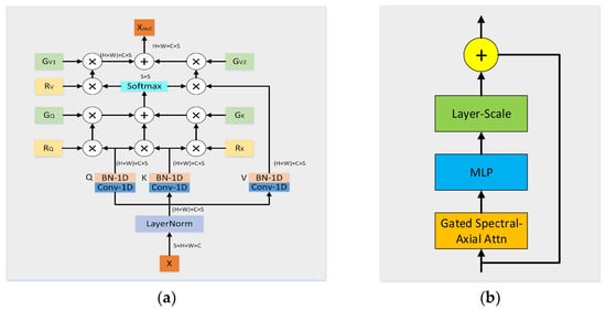
Figure 2. Framework of the proposed GSA. (a) Structure of Gated Spectral-Axial Attention; (b) Structure of GSA Block.

In summary, the spectral–axial attention module is a self-attention mechanism that performs the operation specifically along the spectral axis of the feature map. The formulation of the gated spectral axis incorporates both positional encoding and gating mechanisms.

$${\mathrm{X}}_{out}=\mathrm{softmax}((Q^{T}K+G_Q{Q}^T{R}_Q+G_K{K}^T{R}_K)(G_{V1}V+G_{V2}{R}_V))$$

(13)

where $Q,K,V\in {ℝ}^{(H\times W)\times C\times S}$ denote the linearly projected input $X$ value. $R_Q$, $R_K$, and $R_V$ denote position encoding on Q, K and V, respectively. $G_Q,G_K,G_{V1}\in ℝ$ denote the gate cells on Q, K and V, respectively. $G_{V2}\in ℝ$ denotes the gate cells in the encoding of the position V.

2.3.3. GSA Block

In more complex 3D models, relying solely on the attention mechanism may provide information on certain important features that are not effectively integrated. As shown in Figure 2b, introducing an MLP can help capture and retain this information, thereby avoiding information loss and enhancing the overall effectiveness of the model. Because the 3D input model is extended by an extra dimension, which leads to slow and unstable training during the deep-learning process, we introduce a layer-scale mechanism. LayerScale assigns scaling weights to each feature channel by introducing a learnable diagonal matrix. This approach allows the model to converge to a good result faster at the beginning of training. Compared to fixed scaling factors, the use of learnable parameters allows the model to adapt to the characteristics of different datasets and tasks, thus improving the training efficiency. LayerScale combined with GSA and MLP modules can help the model maintain more information during the feature-embedding process and reduce the effect of redundancy or noise, thereby improving the accuracy and robustness of the final task performance.

3. Results

3.1. Dataset

We used the multidimensional choledoch dataset [32] with 538 pathological images, where the micro-hyperspectral images were acquired using the Micro Hyperspectral Imaging System (MHSI) with a 20× imaging lens. In the original multidimensional choledoch dataset, each hyperspectral image contained 1280 × 1024 pixels in 60 spectral bands. All bands ranged from 550 to 1000 nm. The raw dataset was preprocessed [20], and the spatial dimension size was changed from 1280 × 1024 to 256 × 320. The Ground Truth (GT) of all the images was manually labeled by an experienced pathologist. Across all samples, the annotation masks contained 28,562,510 pixels for normal tissue and 15,510,450 pixels for cancerous tissue.

As shown in Figure 3, the red-labeled areas represent areas of cholangiocarcinoma, and the unlabeled areas were normal. The x- and y-axes show the spatial features of the hyperspectral images, and the z-axis shows the spectral features of the hyperspectral images. Cancerous tissues usually have a higher cell density and larger nuclei than normal tissues, resulting in a greater amount of light being scattered and absorbed within the tissues, thereby reducing overall reflectance. Therefore, the average spectral reflectance value of the cholangiocarcinoma region on the right side of Figure 3 was lower than that of the normal tissue region, particularly in the 550–700 nm band.

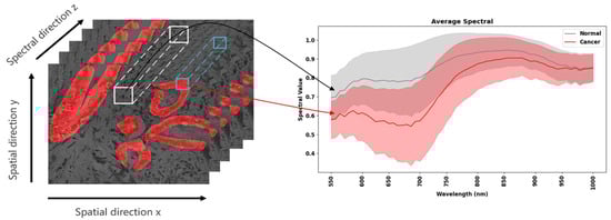
Figure 3. A sample of cholangiocarcinoma from a scenario.

3.2. Implementation Details

To evaluate the proposed method, we use a 4-fold cross-validation approach to rate the performance of the model, with the spatial dimension cropped from 256 × 320 to 192 × 192 and the spectral dimension selected for the first 32 spectral bands. Notably, this dataset was not split at the patch level; rather, the 538 hyperspectral images were divided into four folds. Therefore, there was no information overlap between patches across folds. The standard DynUNet-3d architecture contains six levels and requires multiple spectral bands of 32. However, our dataset did not provide 64 bands. Therefore, to ensure a fair comparison with the baseline model, the input number of the spectral bands was fixed at 32.

The training hyperparameters are listed in Table 1. Owing to GPU memory limitations, we used a batch size of 1. Unless otherwise noted, spectral normalization was applied during the training. We used Adam optimization, where the initial learning rate was 3 × 10⁻³ and the weight decay was 5 × 10⁻⁴. The learning rate scheduler was a cosine annealing restart with an initial annealing period of five, the period multiplication factor was set to two, and the minimum learning rate was 1 × 10⁻⁸. We employed standard data augmentation techniques, including random rotation and flipping, to address the issue of limited sample size. The number of training epochs is limited to 75. All experiments were run in Pytorch and Monai frameworks using an RTX4090 GPU with 24 GB of memory.

Table 1. Parameters of training configuration.

Image Size	Batch Size	Epoch	Optimizer	Learning Rate	LR Scheduler
192 × 192 × 32	1	75	Adam	3 × 10−3	Cosine Annealing restart
Minimum LR	Weight Decay	Initial Annealing Period		Period Factor	Loss function
1 × 10−8	5 × 10−4	5		2	0.5 × Dice + 0.5 × BCE

3.3. Evaluation Metrics

Loss and Evaluation Metric: We used the average loss of dice and BCELoss as the loss of the training process. Dice similarity coefficient (Dice), Intersection over Union (IoU), and Hausdorff Distance (HD) were evaluated.

The correlation formula is as follows:

$$Dice={\displaystyle \frac{2pg}{p+g}}$$

(14)

$${\mathcal{L}}_{\mathrm{Dice}}=1-Dice=1-{\displaystyle \frac{2pg}{p+g}}$$

(15)

$${\mathcal{L}}_{BCE}=-(g\log p+(1-g)\log (1-p))$$

(16)

$$\mathcal{L}={\displaystyle \frac{{\mathcal{L}}_{\mathrm{Dice}}+{\mathcal{L}}_{BCE}}{2}}$$

(17)

$$\mathrm{IoU} = {\displaystyle \frac{TP}{TP+FP+FN}}$$

(18)

$$d_H(X,Y)=\max \{d_{XY},d_{YX}\}=\max \left\{\underset{x\in X}{\max }\underset{y\in Y}{\min }d(x,y),\right.\left.\underset{y\in Y}{\max }\underset{x\in X}{\min }d(x,y)\right\}$$

(19)

$$F={\displaystyle \frac{{({\mu }_{\mathrm{cancer}}-{\mu }_{\mathrm{normal}})}^2}{{\sigma }_{\mathrm{cancer}}^2+{\sigma }_{\mathrm{normal}}^2}}$$

(20)

$$Contrast={\displaystyle \sum _{i,j}{(i-j)}^{2}P(i,j)}$$

(21)

where p represents the sum of the predicted values and g represents the sum of the true values. ${\mathcal{L}}_{\mathrm{Dice}}$ is the Dice loss, which measures the similarity between the predicted binary mask and the true binary mask. ${\mathcal{L}}_{BCE}$ denotes the binary cross-entropy loss, which measures the difference between the predicted value and the true label. TP denotes True Positive, FN denotes False Negative, and FP is False Positive. $d_H(X,Y)$ denotes the Hausdorff Distance between point sets X and Y. $d_{XY}$ denotes the distance between each point x in point set X and each point y in point set Y. The shortest distance was maintained and then determined. This means that for each point x in point set X, calculate its distance to each point y in point set Y, maintain the shortest distance, and then find the largest distance among the shortest distances. $d_{YX}$ denotes the distance from each point y in point set Y to each point x in point set X, maintaining the shortest distance and then finding the largest distance among the shortest distances. ${\mu }_{\mathrm{cancer}}$ and ${\mu }_{\mathrm{normal}}$ represent the mean pixel intensities of cancerous and non-cancerous regions, respectively. ${\sigma }_{\mathrm{cancer}}^2$ and ${\sigma }_{\mathrm{normal}}^2$ are corresponding variances. F denotes the Fisher Score, which quantifies the discriminative ability of a given spectral band to distinguish cancerous from non-cancerous tissues; larger values indicate stronger separability. $P(i,j)$ denotes the probability of co-occurrence of gray levels i and j within a defined spatial relationship derived from the gray-level co-occurrence matrix (GLCM). The term ${(i-j)}^2$ emphasizes the contribution of pixel pairs with high gray-level differences. $Contrast$ denotes the GLCM contrast, which quantifies the spatial texture richness of each image band. Higher values correspond to richer local spatial textures.

3.4. Experimental Results

3.4.1. Analysis of the Results of Hyperspectral Image Segmentation with Different Number of Bands

Hyperspectral images are three-dimensional data consisting of spectral data in multiple bands, which provide rich spectral information useful for pathology image segmentation. By contrast, RGB images contain only three wavelengths (red, green, and blue), which can provide relatively little information. From Table 2, it is clear that the RGB false-color images perform worse than the HSI in image segmentation, and casually, the number of hyperspectral bands increases, and the performance of hyperspectral image segmentation improves. When the number of spectral bands were selected as 60, all three evaluations yielded the best results, with mean values of 60.17%, 73.96% and 81.12 for IoU, Dice, and HD, respectively.

Table 2. Comparison of segmentation performance of False-color images and hyperspectral images of different bands in the DynUnet-2d method (Comparison of results in different spectral bands).

Bands	Method	IoU (%) ↑	Dice (%) ↑	HD (px) ↓
10, 20, 30 (False color image)	DynUNet	59.20 ± 14.54	73.29 ± 12.01	83.73 ± 43.93
1–32 (Hyperspectral image)	DynUNet	59.94 ± 14.72	73.84 ± 12.21	84.00 ± 43.04
1–60 (Hyperspectral image)	DynUNet	60.17 ± 15.18	73.96 ± 12.51	81.12 ± 42.52

Note: ↑ indicates that higher values represent better performance, and ↓ indicates that lower values represent better performance. Bold values indicate the best performance within each column.

3.4.2. Comparison of Semantic Segmentation

As shown in Table 3, we evaluated several 2D segmentation models by inputting hyperspectral images into 2D convolutional networks as multi-channel inputs. The encoder of the UNet-2d model used the pretrained ResNet-34; however, owing to the substantial differences between the RGB and hyperspectral images, direct transfer leads to the poorest performance for UNet-2d. Among these models, DynUNet-2d achieved the best performance among the baseline methods, with an IoU of 59.94%, Dice of 73.84%, and HD of 84.00 px. For 3D models that retain the spectral dimension of hyperspectral images in the input tensor, we observed an overall improved performance compared to their 2D counterparts. Our proposed GSA-Net achieved the best results among all tested models, with an IoU of 60.64%, Dice of 74.44%, and the lowest HD of 76.82 px. Compared to the best-performing 3D baseline (SpecTr), which reached 59.17% IoU, 74.01% Dice, and 78.74 px HD, GSA-Net improved by 1.47% in IoU, 0.43% in Dice, and reduced HD by 1.92 px. Furthermore, compared to DynUNet-3d, GSA-Net showed an average improvement of 3.24% in IoU and 2.86% in Dice while decreasing HD by 10.62 px. These findings confirm the benefit of preserving the spectral context through 3D convolutions and show that the proposed Gated Spectral-Axial Attention mechanism effectively enhances the extraction of spectral dependencies in hyperspectral medical image segmentation.

Table 3. Performance comparison of model segmentation in cholangiocarcinoma dataset (all metric values shown by mean ± standard deviation).

Type	Method	IoU (%) ↑	Dice (%) ↑	HD (px) ↓
2D	Unet-2d [4]	47.01 ± 21.62	60.88 ± 21.25	96.63 ± 46.62
	AttentionUnet-2d [15]	48.35 ± 13.50	64.03 ± 12.74	97.86 ± 46.85
	Kerfoot et al. (2d) [5]	58.62 ± 15.13	72.70 ± 12.82	85.35 ± 44.22
	DynUNet-2d [9]	59.94 ± 14.72	73.84 ± 12.21	84.00 ± 43.04
3D	Unet-3d [4]	48.71 ± 20.80	62.75 ± 20.09	93.92 ± 45.24
	AttentionUnet-3d [15]	50.50 ± 14.63	65.80 ± 13.60	96.54 ± 46.68
	SegResNet (3d) [7]	55.90 ± 14.89	70.48 ± 13.05	84.91 ± 43.60
	SwinUNETR (3d) [8]	56.84 ± 16.22	71.05 ± 14.02	88.75 ± 45.45
	Kerfoot et al. (3d) [5]	57.77 ± 15.93	71.88 ± 13.46	84.11 ± 43.70
	DynUNet-3d [9]	57.40 ± 15.85	71.58 ± 13.59	87.41 ± 44.69
	3D-DDA [12]	57.97 ± 15.42	72.13 ± 12.98	85.21 ± 44.07
	SpecTr [18]	59.17 ± 16.06	73.01 ± 13.33	78.74 ± 43.26
	Ours (GSA-Net)	60.64 ± 14.48	74.44 ± 11.83	76.82 ± 42.77

Note: ↑ indicates that higher values represent better performance, and ↓ indicates that lower values represent better performance. Bold values indicate the best performance within each column.

3.4.3. Computational Complexity and Inference Efficiency of the 3D Model

As shown in Table 4, under our inference setting, GSA-Net uses 2.75 million parameters and 394.9 GFLOPs—slightly fewer than SpecTr (2.82M/402.0G). Despite the comparable FLOPs, it reduces latency from 113.8 ms (SpecTr) to 66.7 ms (−41.3%) and increases FPS from 8.79 to 15.00 (+70.7%), demonstrating the efficiency of the gated spectral–axial module with LayerScale.

Table 4. Complexity and runtime comparison of 3D medical image segmentation models.

Model	Parameters (M)	FLOPs (G)	Latency (ms)	FPS
SegResNet (3d) [7]	1.18	20.9	5.5	180.99
SwinUNETR (3d) [8]	62.19	429.9	52.3	19.13
Kerfoot et al. (3d) [5]	4.81	6.7	3.5	286.79
DynUNet-3d [9]	31.18	269.2	13.4	74.68
3D-DDA [12]	36.18	392.1	45.7	21.87
SpecTr [18]	2.82	402.0	113.8	8.79
Ours (GSA-Net)	2.75	394.9	66.7	15.00

Compared to transformer-heavy SwinUNETR (62.19M parameters, 429.9 GFLOPs), GSA-Net is 95.6% smaller and 8.1% lighter in FLOPs, with similar single-image latency (<70 ms). Lightweight 3D CNNs (e.g., SegResNet-3D, Kerfoot et al.) achieve significantly higher FPS with their low computational costs (6.7–20.9 GFLOPs), while they lose in the accuracy, as shown in Table 3.

Combined with Table 3, we observed that GSA-Net achieved the highest segmentation accuracy among all models compared, while still having a low parameter budget and reasonable throughput. This indicates a better trade-off between accuracy and efficiency compared with SpecTr.

3.4.4. Visualization of Segmentation Results

A visualization of the model segmentation results is shown in Figure 4. The first image in the first row is the false color input (bands 10, 20, and 30) followed by the Ground Truth. The remaining images display the segmentation results from various models, including Unet-2d, AttentionUnet-2d, Kerfoot et al. (2d), DynUNet-2d, Unet-3d, AttentionUnet-3d, SegResNet (3d), SwinUNETR (3d), Kerfoot et al. (3d), DynUNet-3d, 3D-DDA, SpecTr (3d), and GSA-Net. A visual comparison revealed that GSA-Net and SpecTr produced a clearer and more complete segmentation of the target region, with GSA-Net providing more accurate boundary delineation. In contrast, models such as Unet-2d and AttentionUnet-2d struggle with severe artifacts or incomplete structures, highlighting the effectiveness of our Gated Spatial-Axial and Spectral-Axial attention designs over conventional spectral or spatial attention.

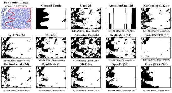
Figure 4. Comparison of the visualized model predictions.

As shown in Figure 5, we select a representative case in which most competing methods perform poorly to highlight the critical role of boundary quality in segmentation. At the interface between cancerous and non-cancerous tissues, the sample exhibited low contrast and high texture similarity. As a result, many methods generate pronounced oversegmentation (invalid regions or false positives) in these areas.

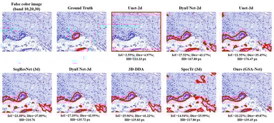
Figure 5. Comparison of segmentation boundaries on a challenging case.

2D networks (e.g., U-Net-2d, DynUNet-2d), which lack an explicit spectral context, tend to misinterpret weak boundaries as continuous tissues. This leads to contour leakage and blotchy false detections, thereby reducing the IoU/Dice and increasing HD. Although typical 3D baselines preserve the spectral dimension, they still produce contiguous false positives or jagged boundaries in texture-similar regions because of the absence of band selection and long-range spectral dependency modeling.

In contrast, GSA-Net employs Gated Spectral–Axial Attention to perform per-band gating and global correlation modeling along the spectral axis, effectively suppressing spurious background responses. Consequently, in this challenging case, GSA-Net significantly reduces invalid regions (improving specificity) while preserving the tumor core, resulting in better boundary adherence and lower HD.

This failure case suggests that simply increasing the spatial resolution is insufficient for handling low-contrast boundaries. Instead, explicit modeling of spectral dependencies is essential for suppressing spurious regions, while maintaining a balance between sensitivity and specificity.

3.4.5. Spectral Band Selection and Analysis

Recent chemometric studies [33,34,35,36,37] emphasize four complementary directions for robust spectral modeling: (i) adaptive calibration to mitigate train–test distribution shifts in multivariate calibration (e.g., MCD-based selection before PLS fitting); (ii) automated preprocessing pipelines that search over de-trending, scatter correction, smoothing, and derivative combinations to remove artifacts while preserving analyte-relevant variance; (iii) data augmentation/generation to enrich scarce calibration sets with realistic spectra paired with concentration values; and (iv) principled variable (wavelength) selection, including sequential/embedded schemes, to improve accuracy and interpretability.

Building on this line of work, our approach allows the deep model to discover informative spectral bands, and we extract the output features from the feature enhancement block located in the first layer of the GSA-Net encoder. These features were then averaged across the batch, channel, and spatial dimensions (i.e., height and width), preserving only the spectral dimension. This process yielded a set of activation values with one scalar per spectral band.

As shown in Figure 6, each fold yields attention activation values for the 32 spectral bands. For each fold, we retain the top 18 bands with the highest activation values. Since the selected bands vary slightly across folds, we further employ an UpSet plot to visualize and analyze the overlap in selected bands across different folds. Figure 7 shows an UpSet plot of the most frequently stimulated spectral channels within 4-fold cross-validation. The intersections between folds were then evaluated to uncover the spectral bands with consistently high activation. As shown, five channels appeared in the four folds, and several others were common in the three folds, demonstrating a strong level of consistency and indicating their significance for learned features.

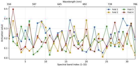
Figure 6. Attention activation values of the 32 spectral bands across the four cross-validation folds.

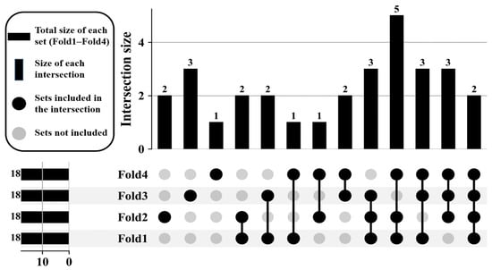
Figure 7. Intersection analysis of the top-activated spectral bands across 4-fold cross-validation.

Figure 8 shows the 16 bands identified by the UpSet intersection analysis as most frequently highlighted by the attention mechanism. These wavelengths span the visible–near-infrared range (550–770 nm) and display two distinct types of discriminative cues.

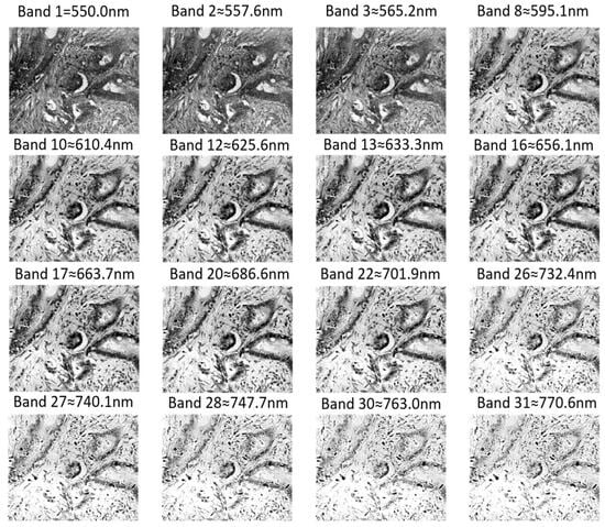
Figure 8. Spatial visualization of the most frequently activated spectral bands in the original hyperspectral image.

To further validate the biological and spatial relevance of these selected bands, we quantified their class-wise spectral separability and spatial texture richness using two complementary metrics: Fisher Score and mean gray-level co-occurrence matrix (GLCM) contrast. Specifically, the Fisher Score evaluates how well each band separates cancerous and non-cancerous tissues at the spectral level, whereas the GLCM contrast captures spatial texture variations within each band.

First, several mid-visible bands—for example, band 12 (625 nm), band 9 (603 nm), and band 11 (616 nm)—exhibit high Fisher scores (0.54–0.55) but relatively low mean GLCM contrast (<1.93 × 10³) (Table 5). This indicates that even though the spatial texture of these bands appears comparatively smooth in the grayscale images, the cancerous and normal tissues show large class-wise spectral differences in mean reflectance, providing strong spectral separability. Therefore, the attention module focuses on these wavelengths primarily because of their characteristic pathological absorption or reflectance signatures, rather than because of conspicuous spatial “inward structures or rich contrasts.”

Table 5. Top-ranked spectral bands by Fisher Score and GLCM Contrast.

Top-Ranked Bands by Fisher Score	Mean Fisher Score	Top-Ranked Bands by GLCM Contrast	Mean GLCM Contrast
Band 12	0.5449	Band 30	3255.84
Band 9	0.5433	Band 31	3243.74
Band 11	0.5428	Band 29	3237.75
Band 13	0.5425	Band 32	3200.30
Band 10	0.5418	Band 28	3146.97
Band 8	0.5386	Band 27	3024.88
Band 14	0.5379	Band 26	2870.91
Band 15	0.5336	Band 25	2712.39
Band 7	0.5316	Band 24	2555.28
Band 16	0.5263	Band 23	2406.89
Band 17	0.5174	Band 22	2273.88
Band 6	0.5156	Band 21	2159.31
Band 18	0.5050	Band 1	2113.37
Band 5	0.5003	Band 20	2058.84
Band 19	0.4890	Band 19	1990.98
Band 4	0.4880	Band 18	1927.03

Conversely, a second group of longer wavelengths, such as bands 28–31 (748–771 nm), show very high GLCM contrast (>3.14 × 10³), while their Fisher scores are moderate. The corresponding images reveal pronounced glandular boundaries and bright–dark transitions, that is, rich spatial contrast and inward structural details. In this spectral band, the spatial texture information draws the attention mechanism, resulting in a high activation value being assigned to it.

The cross-fold activation curves in Figure 6 further confirm that these two types of bands receive consistently elevated attention weights, demonstrating that the model does not simply select bands with the largest mean spectral contrast or richest spatial texture alone. Instead, the learned attention dynamically exploits both types of discriminative information—pure spectral signatures at visible wavelengths and strong spatial structures at selected near-infrared wavelengths.

As shown in Figure 9 and Table 6, although the Top-16 band setup was designed to be the most informative with regard to attention-activated strength and cross-fold consistency, the Full-32 setup outperformed it by a small margin in terms of all metrics (IoU, Dice, and HD). This implies that the other bands not selected in Top-16 still carry additional spectral information that is useful for segmentation.

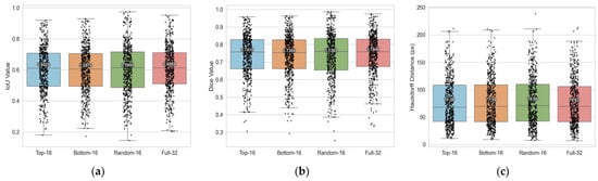
Figure 9. Comparison of segmentation performance across different spectral-band selection strategies. The Boxplots summarize per-case results pooled over the validation sets of all four cross-validation folds: (a) Intersection over Union (IoU), (b) Dice coefficient, and (c) Hausdorff Distance (HD) for Top-16, Bottom-16, Random-16, and Full-32 band inputs.

Table 6. Segmentation performance using top-, bottom-, random-, and full-band selections (mean ± std).

Input Bands	IoU (%) ↑	Dice (%) ↑	HD (px) ↓
Top-16	60.28 ± 14.32	74.18 ± 11.71	77.08 ± 42.98
Bottom-16	59.76 ± 14.84	73.68 ± 12.24	77.59 ± 42.81
Random-16	59.99 ± 16.02	73.69 ± 13.13	78.86 ± 44.80
Full-32	60.64 ± 14.48	74.44 ± 11.83	76.82 ± 42.77

Note: ↑ indicates that higher values represent better performance, and ↓ indicates that lower values represent better performance. Bold values indicate the best performance within each column.

3.4.6. Ablation Study on the GSA Block and Decoder Components

The ablation results in Table 7 show the contributions of each component of the GSA block and the decoder architecture. The baseline (without any component) achieved 55.63% IoU, 70.26% Dice, and 84.75 px HD. When modules are enabled individually, LayerScale yields the largest gain—60.62% IoU and 74.34% Dice) which corresponds to +4.99 percentage points (pp) IoU and +4.08 pp Dice, together with −6.12 px HD relative to the baseline. In comparison, using SPF alone improves accuracy by +0.97 pp IoU/+0.95 pp Dice, and Gated Units alone by +1.03 pp IoU/+0.96 pp Dice. Thus, LayerScale accounts for the majority of single-module improvement (5 pp IoU and 4 pp Dice), which is approximately four to five times greater than the gain achieved by SPF or Gated when used individually.

Table 7. Ablation study of the Gated Spectral-Axial Attention components and the SPF decoder module (all metric values shown by mean ± standard deviation).

Noise Type	Gated Spectral-Axial Attention Block		Decoder	IoU (%) ↑	Dice (%) ↑	HD (px) ↓
	Gated Units	LayerScale	SPF
None	✗	✗	✗	55.63 ± 14.81	70.26 ± 13.06	84.75 ± 44.38
	✗	✗	✔	56.60 ± 14.11 (+0.97)	71.21 ± 12.00 (+0.95)	81.85 ± 42.60 (−2.90)
	✔	✗	✗	56.66 ± 14.32 (+1.03)	71.22 ± 12.34 (+0.96)	81.88 ± 42.19 (−2.87)
	✗	✔	✗	60.62 ± 15.07 (+4.99)	74.34 ± 12.23 (+4.08)	78.63 ± 42.80 (−6.12)
	✔	✗	✔	57.25 ± 14.01 (+1.62)	71.76 ± 11.89 (+1.50)	80.48 ± 42.53 (−4.27)
	✔	✔	✗	60.63 ± 15.25 (+5.00)	74.33 ± 12.39 (+4.07)	77.49 ± 42.74 (−7.26)
	✗	✔	✔	60.63 ± 14.71 (+5.00)	74.41 ± 11.93 (+4.15)	75.79 ± 42.53 (−8.96)
	✔	✔	✔	60.64 ± 14.48 (+5.01)	74.44 ± 11.83 (+4.18)	76.82 ± 42.77 (−7.93)
Gaussian (SNR = 20)	✗	✔	✗	60.61 ± 15.30 (−0.01)	74.31 ± 12.41 (−0.03)	78.21 ± 42.82 (−0.42)
	✔	✔	✔	60.65 ± 14.68 (+0.01)	74.42 ± 12.00 (−0.02)	76.58 ± 42.93 (−0.24)
Gaussian (SNR = 10)	✗	✔	✗	59.98 ± 16.75 (−0.64)	73.57 ± 13.63 (−0.77)	79.99 ± 44.03 (+1.36)
	✔	✔	✔	60.20 ± 16.09 (−0.44)	73.84 ± 13.18 (−0.60)	78.28 ± 43.81 (+1.46)
Gaussian (SNR = 1)	✗	✔	✗	52.30 ± 21.28 (−8.32)	66.06 ± 18.96 (−8,28)	88.36 ± 46.17 (+9.73)
	✔	✔	✔	53.79 ± 20.71 (−6.85)	67.54 ± 18.20 (−6.90)	86.34 ± 45.40 (+9.52)
Gaussian (SNR = 0.1)	✗	✔	✗	50.77 ± 21.77 (−9.85)	64.54 ± 19.69 (−9.80)	90.60 ± 46.54 (+11.97)
	✔	✔	✔	52.55 ± 21.23 (−8.09)	66.30 ± 18.89 (−8.14)	87.92 ± 45.65 (+11.10)

Note: ↑ indicates that higher values represent better performance, and ↓ indicates that lower values represent better performance. “✔” indicates that the corresponding module is included; “✗” indicates that the module is excluded.

Gaussian noise was injected along the spectral dimensions. Consistent with noise-free ablation, LayerScale remains the primary effective factor and is the most stable under noise. At SNR 20 or 10, adding SPF/Gated changes IoU and Dice by no more than 0.1 percentage points, which is practically marginal. When the SNR is 1 or lower, noise-induced degradation outweighs the gains of any single module, indicating that LayerScale alone cannot fundamentally offset the heavy noise. SPF and Gated help counter part of the damage, mainly through slight boundary smoothing; however, their effects are limited and do not fully reverse the degradation.

Compared with using LayerScale alone, adding SPF or Gated leads to negligible changes in IoU and Dice (≤0.10 percentage points) and a reduction in HD of 1.1–2.8 pixels. Because HD emphasizes boundary errors, the effect of these modules manifests primarily as minor boundary adjustments. Under our experimental setup, this magnitude (≈12–34 µm, given 12 µm per pixel in our data) is small with limited practical value while introducing additional model complexity and training cost. Accordingly, we adopted the LayerScale-only variant as the default configuration. Accordingly, we adopted the LayerScale-only variant as the default configuration; in strong-noise scenarios, SPF/Gated may be enabled as optional modules. However, primary robustness still relies on noise-aware training or denoising strategies.

3.4.7. Ablation Study on the Effect of MLP and LayerScale on Convergence

Training instability and slow convergence are major problems in complex 3D architectures with high-dimensional hyperspectral inputs. To mitigate such issues, the LayerScale mechanism introduces a learnable dimension-like matrix to each feature channel, so that the model can scale features dynamically and adapt to task-specific preferences. It not only facilitates fast early convergence but also improves robustness by removing noisy or redundant signals.

As shown in Figure 10, we conducted ablation experiments to compare the effects of MLP and LayerScale on 3D deep feature modeling and convergence behavior. The corresponding training curves are also presented to illustrate the convergence stability. We quantified convergence by the initial slope of the validation curves during the first 30 epochs, where a steeper slope indicates faster convergence, and reported the final performance using Best IoU and Dice. As shown in Table 8, the baseline model achieves 56.92% IoU and 71.36% Dice but exhibits very low early slopes (6.38 × 10⁻⁴ for IoU; 3.82 × 10⁻⁴ for Dice), indicating slow and unstable early-stage learning.

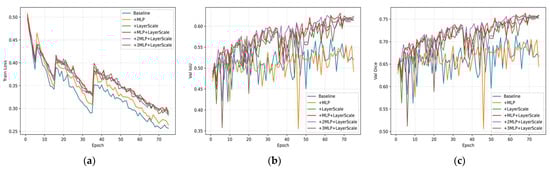
Figure 10. The curves summarize training/validation results across different ablation settings: (a) training loss, (b) validation Intersection over Union (IoU), and (c) validation Dice, over the same 75 training epochs.

Table 8. Effect of LayerScale and MLP on convergence speed and stability.

Module	Best IoU (%)	Early Slope Validation IoU	Best Dice (%)	Early Slope Validation Dice
Baseline	56.92	6.38 × 10−4	71.36	3.82 × 10−4
+MLP	55.49	6.72 × 10−4	70.50	6.44 × 10−4
+LayerScale	62.63	2.61 × 10−3	76.02	2.36 × 10−3
+MLP+LayerScale	63.11	2.75 × 10−3	76.33	2.35 × 10−3
+2MLP+LayerScale	62.57	3.23 × 10−3	75.70	2.67 × 10−3
+3MLP+LayerScale	61.99	3.29 × 10−3	75.70	2.79 × 10−3

Introducing LayerScale alone significantly accelerates and stabilizes training: the early slopes increase to 2.61 × 10⁻³ (IoU) and 2.36 × 10⁻³ (Dice), which are approximately 4.1 times and 6.2 times higher than the baseline, respectively. Final performance also improved to 62.63% IoU and 76.02% Dice, with gains of +5.71 pp and +4.66 pp, respectively. In contrast, using MLP alone leads to only marginal improvement in convergence and even slightly worse final accuracy (55.49% IoU, 70.50% Dice), suggesting that MLP alone does not effectively improve optimization dynamics without LayerScale.

Combining MLP and LayerScale yields the best performance: 63.11% IoU and 76.33% Dice, with fast early slopes (2.75 × 10⁻³ for IoU and 2.35 × 10⁻³ for Dice), representing approximately 4.3 times and 6.1 times the baseline values. Moreover, stacking additional MLP blocks (two or three MLPs with LayerScale) further increases the early slopes to approximately 0.00323–0.00329 for IoU and 0.00267–0.00279 for Dice, which are about 5.1 to 5.2 times and 7.0 to 7.3 times higher than the baseline, respectively. However, this does not lead to improved final accuracy, with the best IoU reaching only 62.57% and 61.99%, and the best Dice remaining at 75.70% in both cases. These results suggest diminishing returns and a potential trade-off in generalization.

LayerScale is the primary contributor to both faster and more stable convergence, with early slopes approximately four to six times steeper than those of the baseline. It also accounts for the majority of the accuracy improvement, contributing an increase of 5–6 percentage points (pp) in IoU and 4–5 pp in Dice. Adding a single lightweight MLP to LayerScale provides the best trade-off between accuracy and computational efficiency. However, stacking two or more MLPs while further accelerating early convergence leads to a slight decline in the final performance, indicating mild over-parameterization for this dataset.

3.4.8. Ablation Study on Attention-Module Substitution

As shown in Table 9, we compared the four attention modules on the same GSA-Net backbone in terms of segmentation performance (excluding PVT), model complexity, and inference efficiency. Our proposed GSA module achieved the best overall performance, with the highest IoU (60.64% ± 14.48) and Dice (74.44% ± 11.83), the fewest parameters (2.75M), the lowest FLOPs (394.9G), and the fastest inference speed (15.00 FPS). Compared to GAA and ViT Self-Attention, GSA not only improves accuracy but also reduces computational cost and increases throughput. Although the FPS values may vary with hardware, the relative ranking demonstrates GSA’s efficiency–accuracy advantage of the GSA.

Table 9. Comparison of alternative attention modules on the same GSA-Net backbone.

Attention Module	IoU (%)	Dice (%)	Params (M)	FLOPs (G)	FPS
ViT	60.12 ± 15.25	73.92 ± 12.46	2.82	402.0	11.02
PVT	-	-	8.50	447.6	11.48
GAA	59.98 ± 14.30	73.94 ± 11.73	3.14	404.9	7.98
GSA (ours)	60.64 ± 14.48	74.44 ± 11.83	2.75	394.9	15.00

4. Discussion

In this study, we investigated the practical utility of Gated Spectral-Axial Attention (GSA) for hyperspectral medical-image segmentation. The proposed GSA-Net incorporates spectral-axis attention within a 3D architecture to effectively model inter-band dependencies and enhance spectral feature discrimination. Our extensive experiments further demonstrate that segmentation-relevant information is not confined to the most salient spectral bands but is distributed across the full spectrum. This highlights the importance of preserving a comprehensive spectral context and justifies the integration of attention-based mechanisms.

Despite the merits of 3D maps in simultaneously representing spectral and spatial information, their computational expense and dependency on large-scale data make them daunting for small- to medium-scale medical tasks. To alleviate these problems, it is necessary to develop lightweight and effective 3D networks designed for hyperspectral data in clinical settings. The high cost and lack of availability of hyperspectral cameras are significant limitations to their widespread use, and post-imaging processing is often required.

Cross-modal learning strategies have immense potential to mitigate the limits of hardware acceleration in HS medical image segmentation for better-quality spectral richness. Using knowledge transfer between various imaging modalities [38,39,40], converting RGB or multispectral input to spectral vectors similar to hyperspectral allows us to replicate the advantages of full-spectrum data without requiring expensive and specialized acquisition devices. This reduces reliance on hyperspectral hardware; however, models can use rich spatial-spectral information, leading to better segmentation accuracy. Such cross-modal generation can also be exploited as a form of data augmentation, and we plan to extend our future work in this regard.

5. Conclusions

Future research directions could include using spectral information to estimate hyperspectral-like representations from commonly acquired data such as RGB, CT, or MRI. Cross-modal spectral reconstruction could potentially lift conventional medical images to bring them near the level of diagnostic richness of hyperspectral data, considering the fine spectral information delivered by the HSI. Brought to broader clinical applications, this approach should allow HSI models of great diagnostic utility to be retrained on more ubiquitous full-spectral HSI data, moving away from reliance upon highly specialized, costly hyperspectral acquisition systems but retaining the benefits of spectrally aware modeling for use in everyday clinical practice.

References

- Gao, S.; Ding, S.; Ho-Ching Iu, H.; Erkan, U.; Toktas, A.; Simsek, C.; Wu, R.; Xu, X.; Cao, Y.; Mou, J. A three-dimensional memristor-based hyperchaotic map for pseudorandom number generation and multi-image encryption. Chaos Interdiscip. J. Nonlinear Sci. 2025, 35, 073105. [Google Scholar] [CrossRef]
- Zeng, W.; Zhang, C.; Liang, X.; Xia, J.; Lin, Y.; Lin, Y. Intrusion detection-embedded chaotic encryption via hybrid modulation for data center interconnects. Opt. Lett. 2025, 50, 4450–4453. [Google Scholar] [CrossRef]
- Liu, Y.; Wang, C.; Lu, M.; Yang, J.; Gui, J.; Zhang, S. From simple to complex scenes: Learning robust feature representations for accurate human parsing. IEEE Trans. Pattern Anal. Mach. Intell. 2024, 46, 5449–5462. [Google Scholar] [CrossRef]
- Ronneberger, O.; Fischer, P.; Brox, T. U-net: Convolutional networks for biomedical image segmentation. In Medical Image Computing and Computer-Assisted Intervention~MICCAI 2015; Springer International Publishing: Munich, Germany, 2015; pp. 234–241. [Google Scholar]
- Kerfoot, E.; Clough, J.; Oksuz, I.; Lee, J.; King, A.P.; Schnabel, J.A. Left-ventricle quantification using residual u-net, Statistical Atlases and Computational Models of the Heart. In Atrial Segmentation and LV Quantification Challenges—9th International Workshop, STACOM 2018; Springer International Publishing: Cham, Switzerland, 2019; pp. 371–380. [Google Scholar]
- Hwang, H.; Rehman, H.Z.U.; Lee, S. 3d u-net for skull stripping in brain mri. Appl. Sci. 2019, 9, 569. [Google Scholar] [CrossRef]
- Myronenko, A. 3d mri brain tumor segmentation using autoencoder regularization. In Brainlesion: Glioma, Multiple Sclerosis, Stroke and Traumatic Brain Injuries~4th International Workshop, BrainLes 2018, Held in Conjunction with MICCAI 2018; Springer International Publishing: Cham, Switzerland, 2019; pp. 311–320. [Google Scholar]
- Hatamizadeh, A.; Nath, V.; Tang, Y.; Yang, D.; Roth, H.R.; Xu, D. Swin unetr: Swin transformers for semantic segmentation of brain tumors in mri images. In International MICCAI Brainlesion Workshop; Springer International Publishing: Cham, Switzerland, 2021; pp. 272–284. [Google Scholar]
- Futrega, M.; Milesi, A.; Marcinkiewicz, M.; Ribalta, P. Optimized u-net for brain tumor segmentation. In International MICCAI Brainlesion Workshop; Springer International Publishing: Cham, Switzerland, 2021; pp. 15–29. [Google Scholar]
- Devlin, J.; Chang, M.W.; Lee, K.; Toutanova, K. Bert: Pre-training of deep bidirectional transformers for language understanding. In Proceedings of the 2019 Conference of the North American Chapter of the Association for Computational Linguistics: Human Language Technologies, Minneapolis, MN, USA, 2–7 June 2019; pp. 4171–4186. [Google Scholar]
- Han, K.; Xiao, A.; Wu, E.; Guo, J.; Xu, C.; Wang, Y. Transformer in transformer. Adv. Neural Inf. Process. Syst. 2021, 34, 15908–15919. [Google Scholar]
- Do, N.T.; Vo-Thanh, H.S.; Nguyen-Quynh, T.T.; Kim, S.H. 3d-dda: 3d dual-domain attention for brain tumor segmentation. In Proceedings of the 2023 IEEE International Conference on Image Processing (ICIP) (IEEE), Kuala Lumpur, Malaysia, 8–11 October 2023; pp. 3215–3219. [Google Scholar] [CrossRef]
- He, K.; Gkioxari, G.; Dollár, P.; Girshick, R. Mask r-cnn. In Proceedings of the IEEE International Conference on Computer Vision, Venice, Italy, 22–29 October 2017; pp. 2961–2969. [Google Scholar] [CrossRef]
- Kido, S.; Hirano, Y.; Hashimoto, N. Detection and classification of lung abnormalities by use of convolutional neural network (cnn) and regions with cnn features (r-cnn). In Proceedings of the 2018 International Workshop on Advanced Image Technology (IWAIT) (IEEE), Chiang Mai, Thailand, 7–9 January 2018; pp. 1–4. [Google Scholar] [CrossRef]
- Oktay, O.; Schlemper, J.; Folgoc, L.L.; Lee, M.; Heinrich, M.; Misawa, K.; Mori, K.; McDonagh, S.; Hammerla, N.Y.; Kainz, B.; et al. Attention u-net: Learning where to look for the pancreas. arXiv 2018, arXiv:1804.03999. [Google Scholar] [CrossRef]
- Chen, Y.; Zhang, F.; Wang, G.; Weng, G.; Fontanelli, D. An Active Contour Model Based on Fuzzy Superpixel Centers and Nonlinear Diffusion Filter for Instance Segmentation. IEEE Trans. Instrum. Meas. 2025, 74, 1–13. [Google Scholar] [CrossRef]
- Lin, T.Y.; Maire, M.; Belongie, S.; Hays, J.; Perona, P.; Ramanan, D.; Dollár, P.; Zitnick, C.L. Microsoft coco: Common objects in context. In Proceedings of the European conference on computer vision, Zurich, Switzerland, 6–12 September 2014; Springer International Publishing: Cham, Switzerland, 2014; pp. 740–755. [Google Scholar]
- Yun, B.; Lei, B.; Chen, J.; Wang, H.; Qiu, S.; Shen, W.; Li, Q.; Wang, Y. Spectr: Spectral transformer for microscopic hyperspectral pathology image segmentation. IEEE Trans. Circuits Syst. Video Technol. 2023, 34, 4610–4624. [Google Scholar] [CrossRef]
- Zhan, G.; Uwamoto, Y.; Chen, Y.W. Hyperunet for medical hyperspectral image segmentation on a choledochal database. In Proceedings of the 2022 IEEE International Conference on Consumer Electronics (ICCE) (IEEE), Nha Trang, Vietnam, 27–29 July 2022; pp. 1–5. [Google Scholar] [CrossRef]
- Zhang, Q.; Li, Q.; Yu, G.; Sun, L.; Zhou, M.; Chu, J. A multidimensional choledochal database and benchmarks for cholangiocarcinoma diagnosis. IEEE Access 2019, 7, 149414–149421. [Google Scholar] [CrossRef]
- Du, D.; Gu, Y.; Liu, T.; Li, X. Spectral reconstruction from satellite multispectral imagery using convolution and transformer joint network. IEEE Trans. Geosci. Remote Sens. 2023, 61, 1–15. [Google Scholar] [CrossRef]
- Zhang, Y.; Wang, Y.; Zhang, B.; Li, Q. A hyperspectral dataset of precancerous lesions in gastric cancer and benchmarks for pathological diagnosis. J. Biophotonics 2022, 15, e202200163. [Google Scholar] [CrossRef]
- Zhang, Y.; Dong, J. Sahis-net: A spectral attention and feature enhancement network for microscopic hyperspectral cholangiocarcinoma image segmentation. Biomed. Opt. Express 2024, 15, 3147–3162. [Google Scholar] [CrossRef]
- Ma, L.; Lu, G.; Wang, D.; Wang, X.; Chen, Z.G.; Muller, S.; Chen, A.; Fei, B. Deep learning based classification for head and neck cancer detection with hyperspectral imaging in an animal model. Proc. SPIE Int. Soc. Opt. Eng. 2017, 10137, 101372G. [Google Scholar] [CrossRef]
- Lin, T.Y.; Dollár, P.; Girshick, R.; He, K.; Hariharan, B.; Belongie, S. Feature pyramid networks for object detection. In Proceedings of the IEEE Conference on Computer Vision and Pattern Recognition, Honolulu, HI, USA, 21–26 July 2017; pp. 2117–2125. [Google Scholar] [CrossRef]
- Liu, Z.; Lin, Y.; Cao, Y.; Hu, H.; Wei, Y.; Zhang, Z.; Lin, S.; Guo, B. Swin transformer: Hierarchical vision transformer using shifted windows. In Proceedings of the IEEE/CVF International Conference on Computer Vision, Virtual, 11–17 October 2021; pp. 10012–10022. [Google Scholar] [CrossRef]
- Han, K.; Wang, Y.; Chen, H.; Chen, X.; Guo, J.; Liu, Z.; Tang, Y.; Xiao, A.; Xu, C.; Xu, Y.; et al. A survey on vision transformer. IEEE Trans. Pattern Anal. Mach. Intell. 2022, 45, 87–110. [Google Scholar] [CrossRef] [PubMed]
- Park, S.; Kim, J.; Kim, J.; Wang, S. Fault Diagnosis of Air Handling Units in an Auditorium Using Real Operational Labeled Data across Different Operation Modes. J. Comput. Civ. Eng. 2025, 39, 04025065. [Google Scholar] [CrossRef]
- Wang, S. Development of approach to an automated acquisition of static street view images using transformer architecture for analysis of Building characteristics. Sci. Rep. 2025, 15, 29062. [Google Scholar] [CrossRef]
- Ho, J.; Kalchbrenner, N.; Weissenborn, D.; Salimans, T. Axial attention in multidimensional transformers. arXiv 2019, arXiv:1912.12180. [Google Scholar] [CrossRef]
- Valanarasu, J.M.J.; Oza, P.; Hacihaliloglu, I.; Patel, V.M. Medical transformer: Gated axial-attention for medical image segmentation. In Medical Image Computing and Computer-Assisted Intervention–MICCAI 2021; Springer International Publishing: Cham, Switzerland, 2021; pp. 36–46. [Google Scholar]
- Wang, Q.; Sun, L.; Wang, Y.; Zhou, M.; Hu, M.; Chen, J.; Wen, Y.; Li, Q. Identification of melanoma from hyperspectral pathology image using 3d convolutional networks. IEEE Trans. Med. Imaging 2020, 40, 218–227. [Google Scholar] [CrossRef]
- Huang, X.; Huang, G.; Chen, X.; Xie, Z.; Ali, S.; Chen, X.; Yuan, L.; Shi, W. An adaptive strategy to improve the partial least squares model via minimum covariance determinant. Chemom. Intell. Lab. Syst. 2024, 249, 105120. [Google Scholar] [CrossRef]
- Chen, X.; Xie, Z.; Tauler, R.; He, Y.; Nie, P.; Peng, Y.; Shu, L.; Ali, S.; Huang, G.; Shi, W.; et al. An automated preprocessing framework for near infrared spectroscopic data. Chemom. Intell. Lab. Syst. 2025, 267, 105542. [Google Scholar] [CrossRef]
- Huang, G.; Zhao, X.; Chen, X.; Ali, S.; Shi, W.; Xie, Z.; Chen, X. Generating spectral samples with analyte concentration values using the adversarial autoencoder. Chemom. Intell. Lab. Syst. 2024, 252, 105194. [Google Scholar] [CrossRef]
- Yeo, C.; Suh, N.; Kim, Y. Fused LassoNet: Sequential feature selection for spectral data with neural networks. Chemom. Intell. Lab. Syst. 2025, 257, 105315. [Google Scholar] [CrossRef]
- Liu, S.; Liu, X.; Wang, S.; Hu, C.; Fang, L.; Yan, X. Dual-Stage Variable Selection: Integrating Static Filtering and Dynamic Refinement for High-Dimensional NIR Analysis. Chemom. Intell. Lab. Syst. 2025, 267, 105533. [Google Scholar] [CrossRef]
- Zhang, J.; Su, R.; Fu, Q.; Ren, W.; He, F.; Nie, Y. A survey on computational spectral reconstruction methods from rgb to hyperspectral imaging. Sci. Rep. 2022, 12, 11051. [Google Scholar] [CrossRef] [PubMed]
- Akhtar, N.; Mian, A. Hyperspectral recovery from rgb images using gaussian processes. IEEE Trans. Pattern Anal. Mach. Intell. 2018, 42, 100–113. [Google Scholar] [CrossRef]
- Shi, Z.; Chen, C.; Xiong, Z.; Liu, D.; Wu, F. Hscnn+: Advanced CNN-based hyperspectral recovery from rgb images. In Proceedings of the IEEE Conference on Computer Vision and Pattern Recognition Workshops, Salt Lake City, UT, USA, 18–23 June 2018; pp. 939–947. [Google Scholar]
Disclaimer/Publisher’s Note: The statements, opinions and data contained in all publications are solely those of the individual author(s) and contributor(s) and not of MDPI and/or the editor(s). MDPI and/or the editor(s) disclaim responsibility for any injury to people or property resulting from any ideas, methods, instructions or products referred to in the content. |
© 2025 by the authors. Licensee MDPI, Basel, Switzerland. This article is an open access article distributed under the terms and conditions of the Creative Commons Attribution (CC BY) license (https://creativecommons.org/licenses/by/4.0/).