Research on Sensorless Control of a Permanent Magnet Synchronous Motor Based on an Improved Sliding Mode Controller with Improved Phase-Locked Loop

Abstract

The ISMC+IPLL (Improved Sliding Mode Control method with Improved Phase-Locked Loop) is proposed to reduce the jitter phenomenon of sensorless control for a permanent magnet synchronous motor (PMSM). Through influence analysis for the structure parameters of SMO to PMSM performance, the basis for determining the switching function and forming coefficient of ISMC+IPLL is constructed. Compared with traditional PI control and anti-integral saturation ASR control, the observation behavior of the ISMC+IPLL under step load and step speed is optimized to varying degrees, which effectively weakens the inherent jitter phenomenon of sensorless control for PMSM and provides a theoretical basis for establishing a high-performance control strategy for PMSM in the whole operation stage.

1. Introduction

Sensorless control technology is a technology that has important value in multiple application areas, and it has achieved cost reduction, system complexity reduction, and manufacturing cost reduction by eliminating dependence on sensors [1]. At the same time, the reliability of the system is improved by reducing the risk of sensor failure due to environmental factors. In addition, sensorless control technology makes the system smaller and lighter, making it ideal for portable devices or space-constrained scenarios. Without sensors, there are fewer potential points of failure and maintenance costs, and less maintenance effort at the same time. Therefore, it is widely used in aerospace, intelligent manufacturing, and other fields, especially in electronic electric drive systems with high requirements for dynamic responses [2].

The application of sensorless control technology in permanent magnet synchronous motors (PMSM) has a number of significant advantages. In terms of design, sensorless PMSM systems are cleaner and easier to install, without regard for installation location and wiring. This control strategy also enhances the flexibility of the system and can integrate into complex automation systems easily. Sensorless vector control has a dynamic performance with fast response and precise speed control. These advantages make sensorless vector-controlled PMSMs suitable for enclosed or difficult-to-maintain environments, and the competitiveness of this motor system in the market has significantly improved with the advancement of technology [3,4].

To achieve sensorless vector control of the PMSM, it is necessary to select a suitable controller in the control structure for speed regulation, while using various types of observers to track rotor position and speed. Several types of speed control strategies are commonly used, including $\mathrm{H}\mathrm{\infty }$ robust control [5], PI control [6], anti-windup automatic speed regulator (ASR) [7], sliding mode control (SMC) [8], predictive current control (PCC) [9], fuzzy logic control (FLC) [10], and artificial neural network (ANN) control [11]. Estimates of PMSM rotor position and speed can be achieved by measuring voltages and currents in a medium to high-speed range. Such observer models have been classified and described in the literature [12], and the main types of observation methods include the Luenberger observer (LO) [13], flux observer (FO) [14], sliding mode observer (SMO) [15], model reference adaptive system (MRAS) [16], extended Kalman filter (EKF) [17], and other types of observers [18]. The speed control and various types of observation methods in the PMSM sensorless vector control structure are described in Table 1, and their advantages and disadvantages are compared.

Table 1. Comparison of different speed control and position detection approaches for sensorless control in PMSM.

Speed Control	Advantages	Disadvantages
$\mathrm{H}\mathrm{\infty }$ robust controller	Suitable for systems with small stability margins Estimating the range of variation in uncertainties Better suppression of system load disturbance Short system settling time	Poor steady-state accuracy Complex drive system design
PI controller	Simple system design Easy to implement in practice Fast system response time	Larger system overshooting Difficult parameter adjustment
Anti-windup ASR controller	Limiting the output to reduce static error Reduces the difficulty of controller parameter adjustment	Slight system overshooting
SMC controller	Insensitive to parameter changes of the controlled object and external disturbance Simple system structure design Smaller system steady-state error Easy system implementation	Inevitable system jitter Slower convergence speed
PCC controller	Simple control algorithm and easy to implement	Relies on the mathematical model of the motor Longer system settling time
FLC controller	Simplifies design complexity for nonlinear time-varying system Does not rely on the exact model of the controlled object Good robustness, adaptability and fault-tolerant capability Short settling time	Unsuitable for complex system control Slight system overshoot
ANN controller	High control performance for complex systems No system overshooting Effectively reduces system steady-state oscillations	System design requires a large number of parameters Difficult to interpret the output
Position detection	Advantages	Disadvantages
Luenberger observer (LO)	Relatively simple algorithm Fast dynamic response and high tracking accuracy	Poor adaptability to motor parameters
Flux observer (FO)	No need for motor speed information, suitable for vector control system without speed sensor	Poor observer performance at low speed Cannot directly detect the flux of the motor rotor
Sliding mode observer (SMO)	Overcomes system uncertainty, strong robustness for disturbances, suitable for PMSM sensorless control Simple algorithm, strong robustness for system parameter changes	System chatter problems from discontinuous switching characteristics
Model reference Adaptive system (MRAS)	Strong robustness for motor parameter changes and external disturbances	Effectiveness of the identification depends on the accuracy of the model parameters
Extended Kalman filter (EKF)	Strong anti-interference capability and adaptive capability in a wide speed range Simple implementation	Reference model accuracy affects observation performance

In sensorless control of PMSM, the forming coefficient (SC) is key to regulating sliding mode control (SMC) performance. For the improved SMO combined with SMC, core switching functions (hyperbolic, saturation, power, sigmoid) all depend on SC to optimize control, such as SC shapes, hyperbolic curve steepness, saturation boundary layer range, and power function piecewise intervals. Improper SC can lead to larger errors, weaker jitter suppression, or slower response. Therefore, exploring the impact of SC on SMC and finding its optimal value is crucial for improving PMSM control accuracy and stability.

It should be emphasized that sensorless control of PMSM is a core technology for high-end equipment, but its traditional control schemes have two major bottlenecks. One is the inherent jitter of the traditional sliding mode observer (SMO) that affects the control accuracy in precision scenarios, and the other is the balance of dynamic and steady-state performance. Aiming at the gaps in existing research such as single-link improvement and lack of collaborative design, the ISMC+IPLL is proposed to reduce the jitter phenomenon of sensorless control for PMSM. The basis for determining the switching function and forming coefficient of ISMC+IPLL is constructed by analyzing the influence on PMSM performance of structure parameters under SMO control. This paper is structured as follows: the process of the implementation of the ISMC+IPLL control strategy is described in Section 2. The models of traditional PI control, anti-windup ASR control, and the ISMC+IPLL control proposed are described in Section 3. The results of the simulation and experimental analysis using different controllers are described in Section 4. The related conclusions are stated in Section 5. The main contributions of this paper are as follows:

(1)

An improved sliding mode control law is derived based on the theory of sliding mode variable structure, and the functional implementation process of the ISMC+IPLL is detailed.

(2)

The system behavior of the ISMC+IPLL control is analyzed with the external conditions and system parameters changing perturbatively, and compared with traditional PI control and anti-windup ASR control.

(3)

The observation ability of the ISMC+IPLL, the traditional SMO for motor rotor position, speed information under different operating conditions, and the suppression effect of system jitter are compared.

(4)

The effects of different switching functions and SC values on the observation performance for ISMC+IPLL are verified, and the experimental results are analyzed and summarized.

2. ISMC+IPLL Control Strategy

Taking the surface-mounted PMSM as an example, the mathematical model of PMSM in the $\alpha \beta$ stationary reference frame is as follows:

$$\left[\begin{array}{c}{\dot{i}}_{\alpha }\\ {\dot{i}}_{\beta }\end{array}\right]={\displaystyle \frac{1}{L_s}}\left[\begin{array}{cc}-R_s& 0\\ 0& -R_s\end{array}\right]\left[\begin{array}{c}{i}_{\alpha }\\ i_{\beta }\end{array}\right]+{\displaystyle \frac{1}{L_s}}\left[\begin{array}{c}{u}_{\alpha }-e_{\alpha }\\ u_{\beta }-e_{\beta }\end{array}\right]$$

(1)

where $u_{\alpha },{ u}_{\beta }$ and $i_{\alpha },{ i}_{\beta }$ are the stator voltages and currents of $\alpha ,\beta$-axis, respectively; $R_s$ is the stator resistance; $L_s=L_d=L_q$, and $L_d,{ L}_q$ are the direct and quadrature axis inductances, respectively; $e_{\alpha },e_{\beta }$ are the back-electromotive force (back-EMF) components of $\alpha ,\beta$-axis, respectively, which can be written as:

$$\left\{\begin{array}{c}{e}_{\alpha }=-{\psi }_f{\omega }_{e}sin{\theta }_e\\ e_{\beta }={\psi }_f{\omega }_{e}cos{\theta }_e\end{array}\right.$$

(2)

where ${\psi }_f={\displaystyle \frac{2}{3}}{\displaystyle \frac{k_t}{p_n}}={\displaystyle \frac{k_e}{p_n}}$ is the flux generated by the rotor permanent magnet, $k_t$ is the constant of motor torque, $k_e$ is the constant of EMF, and $p_n$ is the number of pole pairs, ${\omega }_e$ and ${\theta }_e$ are the rotor electric angular velocity and electric angle, respectively.

From the above, the $e_{\alpha }$ and $e_{\beta }$ contain electromechanical angle and electrical angular velocity information. By designing the current SMO and the normalized PLL to form the ISMC+IPLL, the position information required in PMSM vector control can be effectively obtained, thus realizing sensorless control of the motor.

To address the problem that the linear sliding mode surface is slow in reaching mode, a nonlinear integral sliding mode surface is used to replace the linear one for the design of the ISMC+IPLL. By reasonably selecting the initial state of the integrator, the system is placed on the sliding mode surface at the start, thus reducing the jitter and improving the robustness of the system.

The expression of the integral sliding mode surface is given by:

$$\mathit{s}=c_1\overline{\mathit{i}}+c_2\int \overline{\mathit{i}}dt$$

(3)

where $\mathit{s}={\left[\begin{array}{cc}{s}_{\alpha }& s_{\beta }\end{array}\right]}^T$, $\overline{\mathit{i}}={\left[\begin{array}{cc}{\widehat{i}}_{\alpha }-i_{\alpha }& {\widehat{i}}_{\beta }-i_{\beta }\end{array}\right]}^T$, $c_1>0$, $c_2>0$.

The traditional SMO is designed with an isokinetic reaching law $\dot{s}=-\epsilon sign\left(s\right), \epsilon >0$. To obtain a faster convergence speed and reduce the jitter, the exponential reaching law is chosen to design the SMO of the ISMC+IPLL, which has the general form: $\dot{s}=-\epsilon sign\left(s\right)-ks, \epsilon >0, k>0$.

The rewritten exponential reaching law is:

$$\dot{s}=-\left(k+\zeta \right)f\left(s\right)-ls$$

(4)

where $k, \zeta , l>0$ are the observer gain values and $f\left(s\right)$ is the switching function to be designed.

The expression of the second-order sliding mode observer (SOSMO) using $\alpha , \beta$-axis stator currents as state variables is defined as [19]:

$$\left[\begin{array}{c}{\dot{\widehat{i}}}_{\alpha }\\ {\dot{\widehat{i}}}_{\beta }\end{array}\right]={\displaystyle \frac{1}{L_s}}\left[\begin{array}{cc}-R_s& 0\\ 0& -R_s\end{array}\right]\left[\begin{array}{c}{\widehat{i}}_{\alpha }\\ {\widehat{i}}_{\beta }\end{array}\right]+{\displaystyle \frac{1}{L_s}}\left[\begin{array}{c}{u}_{\alpha }-{\nu }_{\alpha }\\ u_{\beta }-{\nu }_{\beta }\end{array}\right]$$

(5)

where ${\widehat{i}}_{\alpha }, {\widehat{i}}_{\beta }$ are the observed values of the $\alpha , \beta$-axis currents, respectively; ${\nu }_{\alpha },{ \nu }_{\beta }$ are the observer feedback signals.

Differentiating Equation (5) from Equation (1) yields the observer error equation:

$$\left[\begin{array}{c}{\dot{\overline{i}}}_{\alpha }\\ {\dot{\overline{i}}}_{\beta }\end{array}\right]={\displaystyle \frac{1}{L_s}}\left[\begin{array}{cc}-R_s& 0\\ 0& -R_s\end{array}\right]\left[\begin{array}{c}{\overline{i}}_{\alpha }\\ {\overline{i}}_{\beta }\end{array}\right]+{\displaystyle \frac{1}{L_s}}\left[\begin{array}{c}{e}_{\alpha }-{\nu }_{\alpha }\\ e_{\beta }-{\nu }_{\beta }\end{array}\right]$$

(6)

where ${\overline{i}}_{\alpha }$ and ${\overline{i}}_{\beta }$ represent the errors between the observed and measured currents.

The expression for the improved sliding mode control law can be obtained by combining Equations (3), (4) and (6) as follows:

$$\nu ={\displaystyle \frac{L_s}{c_1}}\left[\left(k+\zeta \right)f\left(s\right)+ls\right]+\mu +\left({\displaystyle \frac{c_2{L}_s}{c_1}}-R\right)\overline{i}$$

(7)

where $\mu$ is the constant to be designed.

From Equation (7), when the integral sliding mode signal $\mathit{s}\left(t\right)$ enters the observer, the output feedback signal $\mathit{z}={\left[\begin{array}{cc}{z}_{\alpha }& z_{\beta }\end{array}\right]}^T={\left[\begin{array}{cc}{\nu }_{\alpha }& {\nu }_{\beta }\end{array}\right]}^T$ is obtained by the switching function $f\left(s\right)$.

$$\left[\begin{array}{c}{z}_{\alpha }\\ z_{\beta }\end{array}\right]={\displaystyle \frac{L_s}{c_1}}\left[\left(k+\zeta \right)f\left(\mathit{s}\left(t\right)\right)+l\mathit{s}\left(t\right)\right]+\mu +\left({\displaystyle \frac{c_2{L}_s}{c_1}}-R\right)\overline{\mathit{i}}$$

(8)

where $\mathit{s}\left(t\right)=\left[\begin{array}{c}{s}_{\alpha }\\ s_{\beta }\end{array}\right]=c_1\left[\begin{array}{c}{\overline{i}}_{\alpha }\\ {\overline{i}}_{\beta }\end{array}\right]+c_2\left[\begin{array}{c}\int {\overline{i}}_{\alpha }dt\\ \int {\overline{i}}_{\beta }dt\end{array}\right]$, $\overline{\mathit{i}}=\left[\begin{array}{c}{\overline{i}}_{\alpha }\\ {\overline{i}}_{\beta }\end{array}\right]=\left[\begin{array}{c}{\widehat{\mathit{i}}}_{\mathit{\alpha }}-{\mathit{i}}_{\mathit{\alpha }}\\ {\widehat{\mathit{i}}}_{\mathit{\beta }}-{\mathit{i}}_{\mathit{\beta }}\end{array}\right]$.

To reduce system jitter, four types of continuous switching functions are introduced, as shown in Figure 1.

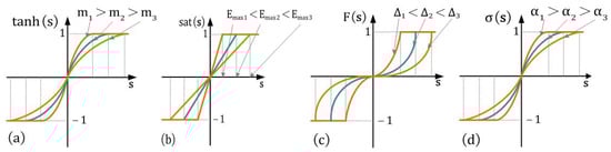
Figure 1. Four types of switching function curves: (a) hyperbolic, (b) saturation, (c) power, and (d) sigmoid.

The hyperbolic function $tanh\left(x\right)$ is defined as follows:

$$f\left(x\right)=tanh\left(x\right)={\displaystyle \frac{e^{mx}-e^{-mx}}{e^{mx}+e^{-mx}}}$$

(9)

where $m$ is the SC of the hyperbolic function, and the different shapes of the hyperbolic function can be constructed by assigning values to the SC. The observer feedback signal $\mathit{z}={\left[\begin{array}{cc}{z}_{\alpha }& z_{\beta }\end{array}\right]}^T$ under the hyperbolic function is:

$$\left[\begin{array}{c}{z}_{\alpha }\\ z_{\beta }\end{array}\right]={\displaystyle \frac{L_s}{c_1}}\left(k+\zeta \right)\left[\begin{array}{c}{\displaystyle \frac{e^{m{s}_{\alpha }}-e^{-m{s}_{\alpha }}}{e^{m{s}_{\alpha }}+e^{-m{s}_{\alpha }}}}\\ {\displaystyle \frac{e^{m{s}_{\beta }}-e^{-m{s}_{\beta }}}{e^{m{s}_{\beta }}+e^{-m{s}_{\beta }}}}\end{array}\right]+{\displaystyle \frac{L_s}{c_1}}l\left[\begin{array}{c}{s}_{\alpha }\\ s_{\beta }\end{array}\right]+\mu +\left({\displaystyle \frac{c_2{L}_s}{c_1}}-R\right)\left[\begin{array}{c}{\overline{i}}_{\alpha }\\ {\overline{i}}_{\beta }\end{array}\right]$$

(10)

The saturation function $sat\left(x\right)$ is defined as follows:

$$f\left(x\right)=sat\left(x\right)=\left\{\begin{array}{c}1, x>E_{max}\\ {\displaystyle \frac{x}{E_{max}}},\left|x\right|\le E_{max}\\ -1,x<-E_{max}\end{array}\right.$$

(11)

where $E_{max}$ is the forming coefficient of the saturation function. The observer feedback signal $\mathit{z}={\left[\begin{array}{cc}{z}_{\alpha }& z_{\beta }\end{array}\right]}^T$ under the saturation function is:

$$\left[\begin{array}{c}{z}_{\alpha }\\ z_{\beta }\end{array}\right]={\displaystyle \frac{L_s}{c_1}}\left(k+\zeta \right)\left[\begin{array}{c}sat\left(s_{\alpha }\right)\\ sat\left(s_{\beta }\right)\end{array}\right]+{\displaystyle \frac{L_s}{c_1}}l\left[\begin{array}{c}{s}_{\alpha }\\ s_{\beta }\end{array}\right]+\mu +\left({\displaystyle \frac{c_2{L}_s}{c_1}}-R\right)\left[\begin{array}{c}{\overline{i}}_{\alpha }\\ {\overline{i}}_{\beta }\end{array}\right]$$

(12)

The segmented power function with variable boundary layer thickness is as follows:

$$f\left(x\right)=F\left(x\right)=\left\{\begin{array}{c}1,x>\Delta \\ {\displaystyle \frac{x\left|x\right|}{{∆}^2}},\left|x\right|\le \Delta \\ -1,x<-\Delta \end{array}\right.$$

(13)

where $\Delta$ is the SC and the boundary layer thickness of the power function. Then the feedback signal $\mathit{z}={\left[\begin{array}{cc}{z}_{\alpha }& z_{\beta }\end{array}\right]}^T$ under the power function is:

$$\left[\begin{array}{c}{z}_{\alpha }\\ z_{\beta }\end{array}\right]={\displaystyle \frac{L_s}{c_1}}\left(k+\zeta \right)\left[\begin{array}{c}F\left(s_{\alpha }\right)\\ F\left(s_{\beta }\right)\end{array}\right]+{\displaystyle \frac{L_s}{c_1}}l\left[\begin{array}{c}{s}_{\alpha }\\ s_{\beta }\end{array}\right]+\mu +\left({\displaystyle \frac{c_2{L}_s}{c_1}}-R\right)\left[\begin{array}{c}{\overline{i}}_{\alpha }\\ {\overline{i}}_{\beta }\end{array}\right]$$

(14)

The sigmoid function is defined as follows:

$$f\left(x\right)=\sigma \left(x\right)={\displaystyle \frac{2}{1+e^{-\alpha x}}}-1$$

(15)

where $\alpha$ is the SC of the sigmoid function. The observer feedback signal $\mathit{z}={\left[\begin{array}{cc}{z}_{\alpha }& z_{\beta }\end{array}\right]}^T$ under the sigmoid function is:

$$\left[\begin{array}{c}{z}_{\alpha }\\ z_{\beta }\end{array}\right]={\displaystyle \frac{L_s}{c_1}}\left(k+\zeta \right)\left[\begin{array}{c}{\displaystyle \frac{2}{1+e^{-\alpha s_{\alpha }}}}-1\\ {\displaystyle \frac{2}{1+e^{-\alpha s_{\beta }}}}-1\end{array}\right]+{\displaystyle \frac{L_s}{c_1}}l\left[\begin{array}{c}{s}_{\alpha }\\ s_{\beta }\end{array}\right]+\mu +\left({\displaystyle \frac{c_2{L}_s}{c_1}}-R\right)\left[\begin{array}{c}{\overline{i}}_{\alpha }\\ {\overline{i}}_{\beta }\end{array}\right]$$

(16)

The sigmoid function has the same mathematical form as the hyperbolic function, which can be used instead of the sigmoid function when it is met: $m=0.5\alpha$.

The speed of the system convergence to the sliding mode surface is also related to the magnitude of the gain value in the reaching law. The fixed synovial gain cannot meet the dynamic performance simultaneously in both reaching mode and sliding mode. Therefore, an algorithm that can adjust the sliding mode gain online under different operating conditions is needed.

From Equation (1), the estimated back-EMF is related to the speed. To reduce the jitter and improve the convergence speed, the following adaptive sliding mode gain algorithm is designed.

$$\zeta =\left\{\begin{array}{c}{\displaystyle \frac{{\omega }_{ref}}{{\omega }_0}}{\zeta }^{\prime },\left|x\right|>\sigma \\ {\displaystyle \frac{\left|\dot{x}\right|}{\left|x\right|+\left|\dot{x}\right|}}·{\displaystyle \frac{{\omega }_{ref}}{{\omega }_0}}{\zeta }^{\prime },\left|x\right|\le \sigma \end{array}\right.$$

(17)

where $\sigma >0$ is the set error limit, ${\omega }_{ref}$ is the reference speed, ${\omega }_0$ is the rated speed, ${\zeta }^{\prime }$ is the reference sliding mode gain, and $x$ is the observation error.

The improved SMO principle of ISMC+IPLL is shown in Figure 2. After the system reaches the sliding mode surface, there is $\mathit{s}={\left[\begin{array}{cc}{s}_{\alpha }& s_{\beta }\end{array}\right]}^T=0$, while $\mathit{i}={\left[\begin{array}{cc}{\overline{i}}_{\alpha }& {\overline{i}}_{\beta }\end{array}\right]}^T=0$, which is brought into Equation (8) to obtain the estimated initial value $\mathit{z}={\left[\begin{array}{cc}{z}_{\alpha }& z_{\beta }\end{array}\right]}^T$ of the back-EMF, and the final estimate $\mathit{e}={\left[\begin{array}{cc}{\widehat{e}}_{\alpha }& {\widehat{e}}_{\beta }\end{array}\right]}^T$ is obtained after LPF.

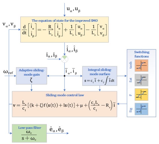
Figure 2. Schematic diagram of the improved SMO for ISMC+IPLL.

The stability of the SMO for ISMC+IPLL is proved by using Lyapunov’s theorem and constructing a Lyapunov function to determine whether the observer remains stable in the equilibrium state $\left(s_{\alpha ,\beta }=0\right)$.

The Lyapunov function is established as:

$$V={\displaystyle \frac{1}{2}}{\mathit{s}}^T\mathit{s}$$

(18)

To ensure the system stability, the Lyapunov condition ${\displaystyle \frac{dV}{dt}}<0$ needs to be met, and the derivative of the Lyapunov function $V_{\alpha ,\beta }$ yields:

$${\displaystyle \frac{ dV}{dt}}={\mathit{s}}^T·\dot{\mathit{s}}$$

(19)

Bringing Equations (3) and (6) into Equation (19) above, the following polynomial is obtained.

$${\displaystyle \frac{dV}{dt}}=\left[\begin{array}{cc}{s}_{\alpha }& s_{\beta }\end{array}\right]\left[\begin{array}{c}{c}_1{\dot{\overline{i}}}_{\alpha }+c_2{\overline{i}}_{\alpha }\\ c_1{\dot{\overline{i}}}_{\beta }+c_2{\overline{i}}_{\beta }\end{array}\right]=\left[\begin{array}{cc}{s}_{\alpha }& s_{\beta }\end{array}\right]\left[\begin{array}{c}{c}_1\left(-{\displaystyle \frac{R_s}{L_s}}{\overline{i}}_{\alpha }+{\displaystyle \frac{1}{L_s}}{e}_{\alpha }-{\displaystyle \frac{1}{L_s}}{\nu }_{\alpha }\right)+c_2{\overline{i}}_{\alpha }\\ c_1\left(-{\displaystyle \frac{R_s}{L_s}}{\overline{i}}_{\beta }+{\displaystyle \frac{1}{L_s}}{e}_{\beta }-{\displaystyle \frac{1}{L_s}}{\nu }_{\beta }\right)+c_2{\overline{i}}_{\beta }\end{array}\right]$$

(20)

Bringing the sliding mode control law expression (7) into the above Equation (20), the stability determination equation is obtained as follows:

$${\displaystyle \frac{dV}{dt}}=\left[\begin{array}{cc}{s}_{\alpha }& s_{\beta }\end{array}\right]\left[\begin{array}{c}{\displaystyle \frac{c_1}{L_s}}\left(e_{\alpha }-\mu \right)-\left\{\left(k+\zeta \right)f\left(s_{\alpha }\right)+l{s}_{\alpha }\right\}\\ {\displaystyle \frac{c_1}{L_s}}\left(e_{\beta }-\mu \right)-\left\{\left(k+\zeta \right)f\left(s_{\beta }\right)+l{s}_{\beta }\right\}\end{array}\right]<0$$

(21)

If the above equation holds, then the following equation is given:

$${\displaystyle \frac{c_1}{L_s}}\left(e_{\alpha }-\mu \right)s_{\alpha }-\left(k+\zeta \right)f\left(s_{\alpha }\right)s_{\alpha }-l{s}_{\alpha }^2+{\displaystyle \frac{c_1}{L_s}}\left(e_{\beta }-\mu \right)s_{\beta }-\left(k+\zeta \right)f\left(s_{\beta }\right)s_{\beta }-l{s}_{\beta }^2<0$$

(22)

According to Lyapunov’s theorem, since $\left|f\left(s_{\alpha ,\beta }\right)\right|\le 1$ and $f\left(s_{\alpha ,\beta }\right)$ have the same sign as $s_{\alpha ,\beta }$, and $k, \zeta , l>0,$ therefore, when the constant $\mu$ to be determined in the SMO satisfies the following relation:

$$\mu >max\left(\left|e_{\alpha }\right|,\left|e_{\beta }\right|\right)$$

(23)

Then there are:

$${\mathit{s}}^T·\dot{\mathit{s}}\le -\left(k+\zeta \right)\left[f\left(s_{\alpha }\right)s_{\alpha }+f\left(s_{\beta }\right)s_{\beta }\right]-l\left(s_{\alpha }^2+s_{\beta }^2\right)\le 0$$

(24)

Therefore, the constant $\mu$ of the improved SMO for ISMC+IPLL must be greater than the magnitude of the $e_{\alpha }$, ${ e}_{\beta }$ to ensure the system stability and thus produce a stable sliding mode motion. When the sliding mode surface function satisfies $\mathit{s}={\left[\begin{array}{cc}{s}_{\alpha }& s_{\beta }\end{array}\right]}^T=0$, its current observation will gradually converge to the actual value, i.e., $\widehat{\mathit{i}}=\mathit{i}$. The control quantity can be obtained from Equation (7) as:

$$\left[\begin{array}{c}{\nu }_{\alpha }\\ {\nu }_{\beta }\end{array}\right]=\left[\begin{array}{c}{\displaystyle \frac{L_s}{c_1}}\left[\left(k+\zeta \right)f\left(s_{\alpha }\right)+l{s}_{\alpha }\right]+\mu +\left({\displaystyle \frac{c_2{L}_s}{c_1}}-R_s\right){\overline{i}}_{\alpha }\\ {\displaystyle \frac{L_s}{c_1}}\left[\left(k+\zeta \right)f\left(s_{\beta }\right)+l{s}_{\beta }\right]+\mu +\left({\displaystyle \frac{c_2{L}_s}{c_1}}-R_s\right){\overline{i}}_{\beta }\end{array}\right]$$

(25)

The high-frequency component is filtered out by the LPF after the traditional SMO has obtained the information of the back-EMF. After filtering to obtain the final estimate, the $arctan$ function or PLL circuit is used to acquire the electrical angle position value from the estimated back-EMF component. In this paper, the latter method is used to obtain position information, and a normalization process is added to the PLL.

The expressions of the position and speed equations can be obtained from the expression of the back-EMF in Equation (1) as:

$$\left\{\begin{array}{c}{\theta }_e=arctan\left(-e_{\alpha }/e_{\beta }\right)\\ {\omega }_e=\sqrt{e_{\alpha }^2+e_{\beta }^2}/{\psi }_f\end{array}\right..$$

(26)

The improved SMO of ISMC+IPLL normalized PLL section is shown in Figure 3.

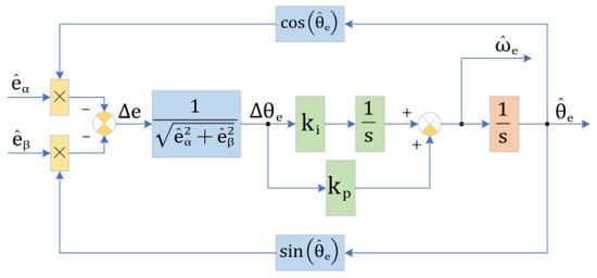
Figure 3. Normalized PLL structure diagram.

After obtaining the back-EMF ${\widehat{e}}_{\alpha },{ \widehat{e}}_{\beta }$, the position error signal of the PLL input can be given as:

$$\Delta e=-{\widehat{e}}_{\alpha }\mathit{cos}{\widehat{\theta }}_e-{\widehat{e}}_{\beta }\mathit{sin}{\widehat{\theta }}_e$$

(27)

Bringing Equation (1) into the above equation yields:

$$\Delta e=E_{ex}\mathit{sin}{\theta }_e\mathit{cos}{\widehat{\theta }}_e-E_{ex}\mathit{cos}{\theta }_e\mathit{sin}{\widehat{\theta }}_e=E_{ex}\mathit{sin}\left({\theta }_e-{\widehat{\theta }}_e\right)$$

(28)

where $E_{ex}={\psi }_f{\omega }_e$. When the observer approaches a steady-state with ${\theta }_e-{\widehat{\theta }}_e\approx 0$, then $\mathit{sin}\left({\theta }_e-{\widehat{\theta }}_e\right)\approx {\theta }_e-{\widehat{\theta }}_e$. The normalization is performed in the system, which is given by Equation (29):

$${\psi }_f{\omega }_e=\sqrt{e_{\alpha }^2+e_{\beta }^2}$$

(29)

Then the position error signal can be approximated as:

$$\Delta {\theta }_e=\mathit{sin}\left({\theta }_e-{\widehat{\theta }}_e\right)\approx {\theta }_e-{\widehat{\theta }}_e$$

(30)

Since the transfer function of the PI regulator is $k_p+{\displaystyle \frac{k_i}{s}}$, the signal $\Delta {\theta }_e$ passes through a PI controller and then through an integrator into an estimated electrical angle ${\widehat{\theta }}_e$, the following equation is obtained:

$$\left({\theta }_e-{\widehat{\theta }}_e\right)·\left(k_p+{\displaystyle \frac{k_i}{s}}\right)·{\displaystyle \frac{1}{s}}={\widehat{\theta }}_e$$

(31)

According to Equation (31), the normalized processing PLL section closed-loop transfer function $G_{PLL}\left(s\right)$ can be obtained as:

$$G_{PLL}\left(s\right)={\displaystyle \frac{{\widehat{\theta }}_e}{{\theta }_e}}={\displaystyle \frac{k_{p}s+k_i}{s^2+k_{p}s+k_i}}$$

(32)

The rotor position error transfer function ${\Phi }_e\left(s\right)$ is:

$${\Phi }_e\left(s\right)={\displaystyle \frac{s^2}{s^2+k_{p}s+k_i}}$$

(33)

When the system is running steadily, the output error is:

$$e_{ss}=\underset{s\to 0}{\mathit{lim}}s·{\displaystyle \frac{1}{s^2}}·{\Phi }_e\left(s\right)=\underset{s\to 0}{\mathit{lim}}{\displaystyle \frac{s}{s^2+k_{p}s+k_i}}=0$$

(34)

From the above Equation (34), the improved PLL can achieve effective tracking of the rotor position, while the observation performance is not affected by the change in speed.

3. ISMC+IPLL Function Implementation

3.1. Traditional PI Control

A PI controller is often used in PMSM vector control, where the input is the difference between the feedback speed ${\omega }_e$ and the reference speed ${\omega }_{ref}$ [20]. The model of the PI controller is represented as $e_0=K_p·e+K_i\int edt$, where $e={\omega }_e-{\omega }_{ref}$. Despite the design being simple, the PI controller cannot regulate when the system parameters change and the load is disturbed. The general structure of PI control is shown in Figure 4.

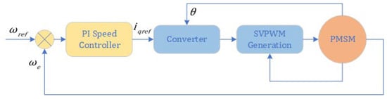
Figure 4. Basic structure of PI controller.

3.2. Anti-Windup ASR Control

Based on the PI control, the anti-windup ASR controller is built to avoid integration saturation by limiting the output of the integrator. The basic structural components of the anti-windup ASR controller and the control flow are given in Figure 5. Although the saturation of the integrator is limited, the controller also becomes slower for the system response and still generates some overshooting.

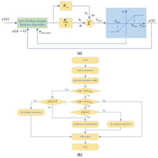
Figure 5. (a) Basic principle of anti-windup ASR controller. (b) Control decision flow diagram of anti-windup ASR controller.

3.3. Proposed ISMC+IPLL Control

The system can make a high-frequency, small-amplitude sliding mode motion along a defined trajectory under certain conditions by using the ISMC+IPLL instead of the PI speed regulator to control the motor. Since the sliding mode is independent of disturbances, the controller has better robustness.

The model of the PMSM in the $d, q$ reference frame is as follows [21]:

$$\left\{\begin{array}{c}{u}_d=R_s{i}_d+L_s{\displaystyle \frac{d{i}_d}{dt}}-{\omega }_e{L}_s{i}_q\\ u_q=R_s{i}_q+L_s{\displaystyle \frac{d{i}_q}{dt}}+{\omega }_e{L}_s{i}_d+{\omega }_e{\psi }_f\end{array}\right.$$

(35)

The equation of mechanical motion of the motor is:

$$\left\{\begin{array}{c}J{\dot{\omega }}_e=p_n{T}_e-p_n{T}_L-B{\omega }_e\\ T_e={\displaystyle \frac{3}{2}}{p}_n{\psi }_f{i}_q\end{array}\right.$$

(36)

where $u_d, u_q$ and $i_d, { i}_q$ are the $dq$-axis components of the stator voltages and currents, respectively; $T_L$ is the loadon the rotor shaft; $B$ is the natural damping coefficient; $J$ is the inertia.

Considering ${\omega }_e=p_n{\omega }_m$, Equation (36) can be rewritten as:

$$J{\dot{\omega }}_m={\displaystyle \frac{3}{2}}{p}_n{\psi }_f{i}_q-B{\omega }_m-T_L$$

(37)

The mechanical angular velocity ${\omega }_m$ is selected as the variable for sliding mode control. Since the control strategy of $i_d=0$ is used, the following Equation (38) can be acquired from Equations (35) and (37).

$$\left\{\begin{array}{c}{\displaystyle \frac{d{i}_q}{dt}}={\displaystyle \frac{1}{L_s}}\left(-R_s{i}_q+u_q-p_n{\psi }_f{\omega }_m\right)\\ {\displaystyle \frac{d{\omega }_m}{dt}}={\displaystyle \frac{1}{J}}\left({\displaystyle \frac{3}{2}}{p}_n{\psi }_f{i}_q-B{\omega }_m-T_L\right)\end{array}\right.$$

(38)

The $x_1$ and $x_2$ are chosen as the state variable of the controller and the state variable expression is written for the PMSM as:

$$\left\{\begin{array}{c}{x}_1={\omega }_{ref}-{\omega }_m\\ x_2={\int }_{-\infty }^t\left({\omega }_{ref}-{\omega }_m\right)dt\end{array}\right.$$

(39)

where ${\omega }_{ref}$ is the reference value of mechanical angular speed; ${\omega }_m$ is the actual value of the mechanical angular speed fed by the observer.

Bringing Equation (38) into Equation (39) yields:

$$\left\{\begin{array}{c}{\dot{x}}_1=-{\dot{\omega }}_m=-{\displaystyle \frac{1}{J}}\left({\displaystyle \frac{3}{2}}{p}_n{\psi }_f{i}_q-B{\omega }_m-T_L\right) \\ {\dot{x}}_2=x_1={\omega }_{ref}-{\omega }_m\end{array}\right.$$

(40)

The sliding mode surface function is chosen as:

$$s=x_1+{cx}_2$$

(41)

Since the system state variables contain the integral term, the initial state of $x_2$ is chosen as:

$$Q_0={\int }_{-\infty }^0{x}_1\left(\xi \right)d\xi =-{\displaystyle \frac{x_0}{c}}$$

(42)

where $c>0$ is the integration constant; $x_0$ is the initial state of $x_1$, and $Q_0$ is the initial state of the variable $x_2$.

The derivative of the expression (41) yields:

$$\dot{s}={\dot{x}}_1+c{\dot{x}}_2={\dot{x}}_1+c{x}_1$$

(43)

To ensure that the system has a fast convergence speed, the controller is designed based on the exponential reaching law and the saturation function, and the sliding mode surface should satisfy the following reaching law.

$$\left.\begin{array}{c}\dot{s}=-\epsilon sat\left(s\right)-qs\\ sat\left(s\right)=\left\{\begin{array}{c}1,s>E_{max}\\ {\displaystyle \frac{s}{E_{max}}},\left|s\right|\le E_{max}\\ -1,s<-E_{max}\end{array}\right.\end{array}\right\}$$

(44)

where $\epsilon , q>0$; $E_{max}$ is the boundary thickness of the saturation function.

Combining Equations (41), (43) and (44) yields the following expression:

$$\dot{s}={\dot{x}}_1+c{x}_1=-\epsilon sat\left(s\right)-qs$$

(45)

The expression under the exponential reaching law is obtained as follows:

$$i_q\left(t\right)={\displaystyle \frac{2J}{3p_n{\psi }_f}}\left[c{x}_1+{\displaystyle \frac{B}{J}}{\omega }_m+{\displaystyle \frac{T_L}{J}}+\epsilon sat\left(s\right)+qs\right]$$

(46)

The ISMC+IPLL controller simulation model is shown in Figure 6.

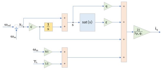
Figure 6. Block diagram of the ISMC+IPLL controller.

If the disturbance error $d_{error}\left(t\right)$ is considered, the derivative of the system sliding mode surface is:

$$\dot{s}\left(t\right)={\dot{x}}_1\left(t\right)+c{x}_1\left(t\right)+d_{error}\left(t\right)$$

(47)

The controller function under disturbance is obtained as:

$$i_q\left(t\right)={\displaystyle \frac{2J}{3p_n{\psi }_f}}\left[c{x}_1+{\displaystyle \frac{B}{J}}{\omega }_m+{\displaystyle \frac{T_L}{J}}+\epsilon sat\left(s\right)+qs+d_{error}\right]$$

(48)

Since the $d_{error}\left(t\right)$ is an unknown disturbance term that is introduced, it is essential to calibrate its upper and lower bounds and write the expression of the exponential reaching law. Let $d_{Lower}\le d_{error}\left(t\right)\le d_{Upper}$, so that $d_{actual}\left(t\right)$ is the determined value of the disturbance term, then the reaching law can be acquired as:

$$\dot{s}=-\epsilon sat\left(s\right)-qs+d_{actual}\left(t\right)-d_{error}\left(t\right)$$

(49)

To satisfy the stability condition, a positive definite Lyapunov function is constructed as $V={\displaystyle \frac{1}{2}}{s}^2\ge 0, s\ne 0$, and after the derivation this yields:

$$\dot{V}=s·\dot{s}=-\epsilon s·sat\left(s\right)-q{s}^2+\left[d_{actual}\left(t\right)-d_{error}\left(t\right)\right]s<0$$

(50)

If $s>0$, then $d_{actual}\left(t\right)=d_{Lower}$ can be taken, and if $s<0$, then $d_{actual}\left(t\right)=d_{Upper}$ can be taken. Combining the above gives the determined value of disturbance as follows:

$$d_{actual}\left(t\right)={\displaystyle \frac{d_{Upper}+d_{Lower}}{2}}-{\displaystyle \frac{d_{Upper}-d_{Lower}}{2}}sign\left(s\right)$$

(51)

The expression of the $q$-axis current under disturbance can be given as:

$$i_q\left(t\right)={\displaystyle \frac{2J}{3p_n{\psi }_f}}\left[c{x}_1+{\displaystyle \frac{B}{J}}{\omega }_m+{\displaystyle \frac{T_L}{J}}+\epsilon sat\left(s\right)+qs+d_{actual}\left(t\right)\right]$$

(52)

By selecting the appropriate parameter values $c, \epsilon$, and $q$, the $q$-axis reference current $i_{qref}$ can be solved quickly using the improved ISMC. In the exponential reaching law, to ensure fast convergence while weakening the system jitter, the $\epsilon$ should be reduced while increasing $q$.

4. Analysis of Simulation and Experiment

The proposed ISMC+IPLL control is compared with the traditional PI control and the anti-windup ASR control, and the effectiveness of the strategy is verified by simulation and experiment; the system behavior under different controllers is also analyzed. The structure diagram of sensorless vector control under different controller modes is given in Figure 7.

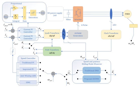
Figure 7. Structure of sensorless vector control of PMSM in different controller modes.

4.1. Simulation Results

The main parameters and the control coefficients used in the simulation process are defined in Table 2. The controller behavior is compared under step changes in load and speed by building simulation models of different controllers in MATLAB/Simulink 2024b. Moreover, to compare the fault-tolerance ability, the control performance of different controllers is verified when the load and speed are disturbed.

Table 2. Main simulation parameters of PMSM used in MATLAB/Simulink.

PMSM Parameters	Value	PMSM Parameters	Value
Rated voltage/V	200	Rated speed/rpm	3000
Rated torque/N·m	10	Peak current/A	30
Moment of inertia J/kg·m2	0.0034	Number of pole pairs ${\mathrm{p}}_{\mathrm{n}}$	4
Stator phase resistance Rs/Ω	0.045	Direct inductance $L_d$/mH	0.235
Flux amplitude of the permanent magnets ${\psi }_f$/Wb	0.048517	Quadratic inductance $L_q$/mH	0.235
SVPWM switching frequency $f$/kHz	10	SVPWM control coefficient	0.9
Cut-off frequency of the LPF ${\omega }_c$/Hz	500

4.1.1. Analysis of Controller Behavior Under Step Load Change

To ensure the objectivity of the comparative experiment, the test device applies load torque to the rotor shaft in a timed and quantitative manner. Specifically, a step load torque of 0 N·m to 6 N·m is applied at 0.8 s, and the load is removed at the preset time when necessary (e.g., a 0.6 N·m load is added at 0.4 s and removed at 0.8 s in subsequent observer performance tests). This loading method avoids randomness in load application and ensures that the response differences of different controllers are only caused by their own control characteristics, rather than inconsistent load conditions.

Figure 8 shows the system response for different controllers under step load change from 0 to 6 N·m at 0.8 s and gives the comparative relationship between the torque $T_e$ and speed $n$ of the system. Dynamic and steady-state evaluation indexes are given for the dynamic response of different controllers, including rise time ($T_r$), peak time ($T_p$) and peak overshoot (${\sigma }_p$) and steady-state error ($E_{ss}$). The results of torque and speed response for traditional PI, improved PI, anti-windup ASR, and the ISMC control proposed in this paper under sudden changes in load are summarized in Table 3. From the table, it can be seen that the traditional PI controller shows the worst performance in terms of speed response at startup and torque response when the load suddenly changes. After parameter optimization, the steady-state error of the improved PI controller decreases from 6.59 rpm to 0.06 rpm. The steady-state error of torque and overshoot are smaller than those of the traditional PI and anti-windup ASR controllers after the abrupt load change.

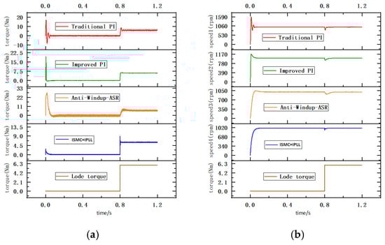
Figure 8. (a) Torque response of different controllers under step change in load torque. (b) Speed response of different controllers under step change in load torque.

Table 3. System behavior under step change in load torque.

Controller Category	Torque Response (N·m)
	${\mathbf{T}}_{\mathbf{r}}\left(\mathbf{s}\right)$	${\mathbf{T}}_{\mathbf{p}}\left(\mathbf{s}\right)$	${\mathbf{E}}_{\mathbf{s}\mathbf{s}}$	${\mathbf{\sigma }}_{\mathbf{p}}$
Traditional PI	0.006	0.012	1.11	2.98
Improved PI	0.005	0.011	0.06	0.43
Anti-windup-ASR	0.031	0.068	0.78	2.08
ISMC+IPLL	0.0004	0.001	0.11	2.96
Controller Category	Speed Response (rpm)
	${\mathbf{T}}_{\mathbf{r}}\left(\mathbf{s}\right)$	${\mathbf{T}}_{\mathbf{p}}\left(\mathbf{s}\right)$	${\mathbf{E}}_{\mathbf{s}\mathbf{s}}$	${\mathbf{\sigma }}_{\mathbf{p}}$
Traditional PI	0.006	0.011	6.59	579
Improved PI	0.007	0.009	0.06	168
Anti-windup-ASR	0.042	0.062	0.81	41
ISMC+IPLL	0.148	——	0.35	——

Although the overshoot for the speed response of the anti-windup ASR controller is only 41 rpm, the load torque shows serious jitter throughout the whole stage. The ISMC+IPLL controller has no overshoot in speed at startup, and the starting torque is much smaller than the other three types of controllers. The speed rise time of the ISMC+IPLL controller reaches 0.148 s at startup without overshoot, but the torque response time is only 0.0004 s when the load changes abruptly, which indicates that the torque tracking performance of the ISMC+IPLL controller is better than that of the other three types under an abruptly changing load.

4.1.2. Analysis of Controller Behavior Under Dynamic Changes in Load

Figure 9 shows the torque and speed response using different controllers under dynamic load changes. The dynamic load change experiment adopts a staged loading strategy. The load torque is adjusted from 1 N·m to 4 N·m, 5 N·m, 7 N·m, and 3 N·m at 0.4 s, 0.6 s, 0.8 s, and 1.0 s, respectively. The load is applied by the torque loading module of the experimental platform, which realizes precise torque control through the closed-loop adjustment of the motor drive system, ensuring that the load amplitude and timing meet the experimental design requirements. The specific results of the dynamic and steady-state evaluation indexes at startup for the four different controllers are given in Table 4.

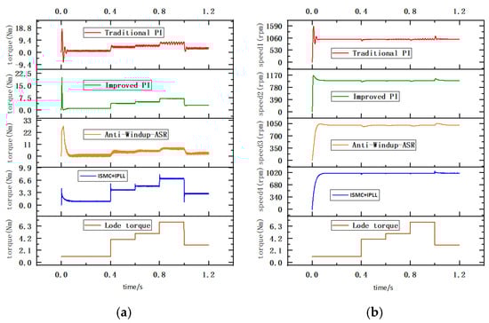
Figure 9. (a) Torque response of different controllers under dynamic changes in load torque. (b) Speed response of different controllers under dynamic changes in load torque.

Table 4. System behavior under dynamic change in load torque.

Controller Category	Torque Response (N·m)
	${\mathbf{T}}_{\mathbf{r}}\left(\mathit{s}\right)$	${\mathbf{T}}_{\mathbf{p}}\left(\mathit{s}\right)$	${\mathbf{E}}_{\mathbf{s}\mathbf{s}}$	${\mathbf{\sigma }}_{\mathbf{p}}$
Traditional PI	0.0005	0.005	0.65	16.74
Improved PI	0.0009	0.005	0.061	18.96
Anti-windup-ASR	0.0012	0.018	1.197	25.99
ISMC+IPLL	0.0004	0.0014	0.076	3.364
Controller Category	Speed Response (rpm)
	${\mathbf{T}}_{\mathbf{r}}\left(\mathit{s}\right)$	${\mathbf{T}}_{\mathbf{p}}\left(\mathit{s}\right)$	${\mathbf{E}}_{\mathbf{s}\mathbf{s}}$	${\mathbf{\sigma }}_{\mathbf{p}}$
Traditional PI	0.0065	0.012	7.94	575.5
Improved PI	0.0068	0.011	0.004	158.1
Anti-windup-ASR	0.046	0.064	1.001	34.27
ISMC+IPLL	0.139	——	0.421	——

From the figure, it can be seen that the improved ISMC+IPLL controller has a better torque response than the other three types of controllers at startup, and the steady-state error and overshoot of torque are only 0.076 N·m and 3.364 N·m.

4.1.3. Analysis of Controller Behavior Under Disturbance in Load and Speed

To verify the fault tolerance of the proposed ISMC+IPLL, different levels of external disturbances are introduced when the load and reference speed change, and the tracking ability of the system under different controller modes in load and speed disturbance are discussed. The load changes from 1 N·m to 7 N·m at 0.6 s when the external disturbances introduced in the system, from 5% to 15% of the rated torque. The comparative results of the torque and speed jitter values for different levels of load disturbance in different controller modes are given in Table 5. The behavior of the system torque and speed response is shown in Figure 10, when a 10% load disturbance is introduced.

Table 5. System behavior under different levels of disturbances in load torque.

Controller Category	Torque Response (N·m)
	0%	5%	10%	15%
Traditional PI	1.1815	1.2195	1.353	1.411
Improved PI	0.0705	0.2415	0.423	0.629
Anti-windup-ASR	1.128	1.178	1.199	1.215
ISMC+IPLL	0.155	0.3095	0.625	0.882
Controller Category	Speed Response (rpm)
	0%	5%	10%	15%
Traditional PI	26.561	28.854	34.11	40.65
Improved PI	0.0365	3.5555	6.841	10.46
Anti-windup-ASR	1.136	1.618	1.858	2.241
ISMC+IPLL	1.365	3.855	7.567	11.78

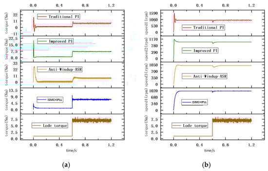
Figure 10. (a) Torque response of different controllers under 10% disturbance in load torque. (b) Speed response of different controllers under 10% disturbance in load torque.

As shown in Figure 10, the dynamic tracking performance of the controller experienced varying degrees of distortion after introducing load disturbances. The fault tolerance for load disturbances under 10% disturbance of traditional PI controllers is far inferior to that of other types of controllers, with fluctuation values of torque and speed response reaching 1.353 N m and 34.11 rpm, respectively. The improved PI controller and the ISMC+IPLL controller have better torque tracking ability for load disturbance than the other two types of controllers, and the best performance for speed tracking is shown by the anti-windup ASR controller, where the maximum speed fluctuation is only 1.858 rpm under 10% disturbance. Although there is not much difference in the tracking performance of torque and speed between the improved PI and the ISMC+IPLL, the ISMC+IPLL can quickly return to the reference value when the load changes suddenly, and its comprehensive dynamic performance is better than that of other types of controllers.

Table 6 shows the comparison of the torque and speed jitter for different controllers when the disturbances occur at reference speed. The initial speed is set to 1000 rpm, and the reference speed is disturbed in different levels at 0.6 s. Figure 11 shows the behavior of the torque and speed response under 15% speed disturbance. From the figure, it can be seen that, when different levels of disturbances are introduced in the reference speed, the improved PI controller shows worse tracking performance for torque and speed than the anti-windup ASR and ISMC+IPLL controllers, with speed fluctuation error reaching 89.35 rpm under 15% speed disturbance. The torque fluctuation of the ISMC+IPLL controller is much smaller than that of the other controllers at different levels of disturbance, and the maximum torque jitter is only 0.243 N·m, even under 15% disturbance in speed. Meanwhile, the speed fluctuation value of the ISMC+IPLL controller is the smallest, with a value of only 12.59 rpm, which indicates that the designed ISMC+IPLL controller can achieve stable tracking of load and reference speed when the rated parameters of the system are disturbed.

Table 6. System behavior under different levels of disturbances in reference speed.

Controller Category	Torque Response (N·m)
	0%	$5\mathbf{\%}$	10%	15%
Traditional PI	0.644	1.167	2.458	3.011
Improved PI	0.068	3.096	4.505	6.151
Anti-windup-ASR	1.422	1.7985	2.847	3.757
ISMC+IPLL	0.1045	0.1155	0.168	0.243
Controller Category	Speed Response (rpm)
	0%	5%	10%	15%
Traditional PI	7.9755	29.629	54.81	77.39
Improved PI	0.046	27.616	54.95	89.35
Anti-windup-ASR	1.366	7.911	12.09	16.47
ISMC+IPLL	1.166	4.4375	8.169	12.59

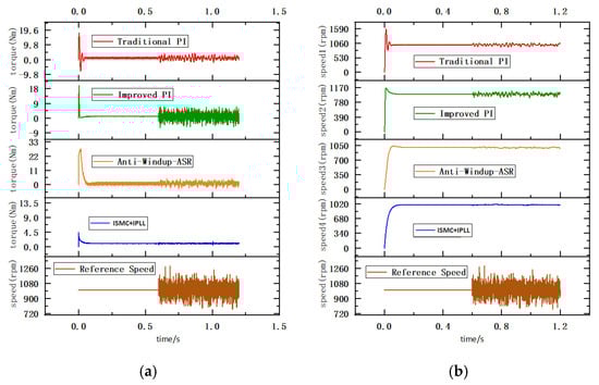
Figure 11. (a) Torque response of different controllers under 15% disturbance in reference speed. (b) Speed response of different controllers under 15% disturbance in reference speed.

4.1.4. System Behavior of ISMC+IPLL Control

Figure 12 shows the system behavior of the optimal ISMC+IPLL control under different conditions. The response under different conditions is presented in Figure 12a–d, and the same arrangement is used for all picture results.

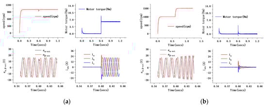
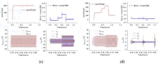
Figure 12. (a) System behavior of ISMC+IPLL control under step load. (b) System behavior under step change in reference speed. (c) System behavior under dynamic changes in load. (d) System behavior under dynamic changes in reference speed.

(1)

The upper left picture shows the speed response curve during the whole process.

(2)

The upper right picture shows the torque tracking curve under different conditions.

(3)

The bottom left picture shows the estimated curve of the rotor back-EMF ${\widehat{\mathrm{e}}}_{\alpha },{\widehat{\mathrm{e}}}_{\beta }$ in a definite time range after LPF filtering.

(4)

The bottom right picture shows the response curve of the three-phase current ${\mathrm{i}}_{\mathrm{a}\mathrm{b}\mathrm{c}}$ when the load and reference speed change.

Figure 12a shows the system response behavior under the step load. The load is changed from 0 N·m to 6 N·m at 0.6 s. From the figure, it can be seen that the speed shows a certain drop when the load increases instantly, but it is still able to return to the reference value in a short time. The torque response of the system shows some overshoot at startup and time in load changing, but the overall tracking ability for load torque is good. The estimated back-EMF ${\widehat{\mathrm{e}}}_{\alpha },{\widehat{\mathrm{e}}}_{\beta }$ does not show a large fluctuation at 0.55–0.65 s, and only a small waveform drop phenomenon occurs at 0.6 s. The three-phase current $i_{abc}$ can be quickly adjusted and achieves stability after the load changes abruptly.

Figure 12b shows the system behavior when the reference speed changes from 1000 to 1500 rpm. From the figure, it can be seen that the system torque $T_e$ and three-phase current $i_{abc}$ both produce a certain fluctuation when the speed changes, but they can return to the reference value in a short time. The amplitude of the estimated back-EMF ${\widehat{\mathrm{e}}}_{\alpha },{\widehat{\mathrm{e}}}_{\beta }$ will become larger, consequently, due to the increase of the reference speed, which causes the waveform frequency to become faster and allows the SMO to effectively track the rotor at high speed.

Figure 12c shows the response of the system when the load is 20%, 50%, and 100% of the rated value. Despite the load changing continuously, the effect on speed and torque is slight, while the three-phase current ${\mathrm{i}}_{\mathrm{a}\mathrm{b}\mathrm{c}}$ can produce a stable tracking waveform under different levels of load.

Figure 12d shows the behavior of the system under dynamic changes in the reference speed. The reference value increases from 500 rpm to 800 rpm at 0.4 s, increases to 1000 rpm after 0.6 s and then decreases to 300 rpm at 0.8 s. The system torque and three-phase current $i_{abc}$ fluctuate at the moment when the reference speed value changes. In the process of reference speed increase, the waveform amplitude and frequency of the estimated back-EMF ${\widehat{\mathrm{e}}}_{\alpha },{\widehat{\mathrm{e}}}_{\beta }$ observed by SMO of ISMC+IPLL can accurately track the change of speed due to the adaptive sliding mode gain algorithm; this enables the ISMC+IPLL controller to still demonstrate good control performance under different operating conditions.

4.1.5. Comparison of the Observed Performance of Improved SMO for ISMC+IPLL and Traditional SMO

(a)

Comparison of observation performance under step load

The initial speed is set to 418 rad/s, and the 0.6 N·m load is added at 0.4 s and removed at 0.8 s. The observation results of the traditional SMO and the improved SMO for ISMC+IPLL under three different types of controllers are given in Table 7. The rise time ${\mathrm{T}}_{\mathrm{r}}$ and the steady-state error $E_{ss}$ after speed stabilization are used as evaluation indexes for rotor speed tracking. After the system parameters stabilize, the jitter of the observer in tracking speed and position errors is used as the main observation indicator, including the speed tracking error jitter value $\overline{\Delta {\omega }_{\mathrm{e}}}$ and the position tracking error jitter value $\overline{\Delta {\theta }_{\mathrm{e}}}$.

Table 7. Comparison of SMO observation performance under step load.

Experiment	Controller	Traditional SMO				Improved SMO
		${\mathbf{T}}_{\mathbf{r}}\left(\mathbf{s}\right)$	${\mathbf{E}}_{\mathbf{s}\mathbf{s}}$	$\overline{\mathbf{\Delta }{\omega }_{\mathbf{e}}}$	$\overline{{\mathbf{\Delta }\mathbf{\theta }}_{\mathbf{e}}}$	${\mathbf{T}}_{\mathbf{r}}\left(\mathbf{s}\right)$	${\mathbf{E}}_{\mathbf{s}\mathbf{s}}$	$\overline{\mathbf{\Delta }{\mathbf{\omega }}_{\mathbf{e}}}$	$\overline{\mathbf{\Delta }{\mathbf{\theta }}_{\mathbf{e}}}$
A	Traditional PI	0.076	8.176	14.06	0.0674	0.096	4.699	9.3115	0.056
B	Anti-windup-ASR	0.090	3.496	3.566	0.0417	0.096	1.587	2.0658	0.032
C	ISMC+IPLL	0.124	6.835	7.576	0.0476	0.125	3.417	4.9997	0.042

Figure 13, Figure 14 and Figure 15 show the observed behavior curves of the traditional SMO and improved SMO under traditional PI control, anti-windup ASR control, and the ISMC+IPLL control mode designed in this paper, respectively. The left figure shows the tracking curve of rotor speed by traditional SMO and improved SMO, and the right figure shows the rotor position observation error curve. The same level of step load is added and removed at the same time to ensure the reliability of the observations. From Table 7 it can be seen that, although the tracking performance of the traditional SMO and the improved SMO for rotor speed and position in the anti-windup ASR controller mode are better than the other two types of controllers, the steady-state errors $E_{ss}$ of the speed tracking after reaching the reference speed are 3.496 rad/s and 1.587 rad/s, respectively. The speed tracking curves of the ISMC+IPLL controller do not overshoot under either the traditional SMO or the improved SMO, and the tracking error jitter values $\overline{{\Delta \theta }_{\mathrm{e}}}$ for the rotor position are not much different, compared to the anti-windup ASR control mode.

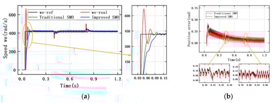
Figure 13. (a) Tracking curve for rotor speed of traditional PI controller under step load. (b) Rotor position observation error curve of traditional PI controller under step load.

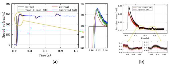
Figure 14. (a) Tracking curve for rotor speed of anti-windup ASR controller under step load. (b) Rotor position observation error curve of anti-windup ASR controller under step load.

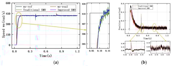
Figure 15. (a) Tracking curve for rotor speed of ISMC+IPLL controller under step load. (b) Rotor position observation error curve of ISMC+IPLL controller under step load.

Compared with the observation results of the traditional SMO, the rise time $T_r$ of the improved SMO for ISMC+IPLL is larger, which is mainly due to the adaptive sliding mode gain control strategy used in the improved SMO for ISMC+IPLL. The gain value of the improved SMO is much smaller than the traditional SMO at the low speed, which leads to a larger rise time $T_r$, but the steady-state error $E_{ss}$ and the tracking error jitter values $\overline{{\Delta \omega }_e}$ and $\overline{{\Delta \theta }_e}$ after the system reaches the reference speed are smaller than the traditional SMO. The comparative results of SMO average observation error ${\Delta \omega }_e$ and ${\Delta \theta }_e$ for different controllers under step load are given in Figure 16. From the figure, it can be seen that the observation performance of the traditional SMO and the improved SMO for ISMC+IPLL control mode are better than the other two types of controllers. The average observation errors of the traditional SMO for speed and position are −1.24633 rad/s and 0.057 rad, respectively, while the average observation errors of the improved SMO are only −0.504 rad/s and 0.044 rad. Therefore, compared with the traditional SMO using the fixed gain, the tracking performance of the proposed improved SMO under step load is enhanced, and the jitter inherent in the traditional observer can be more effectively suppressed.

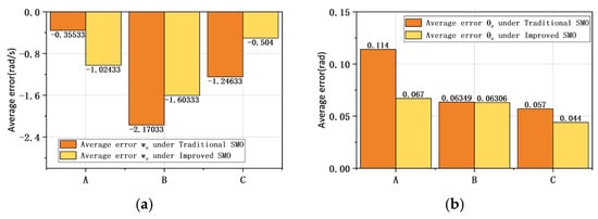
Figure 16. A-PI control. B-anti-windup ASR control. C-ISMC+IPLL control. (a) Average observation error ${\Delta \omega }_{\mathrm{e}}$ of SMO for different controllers under step load. (b) Average observation error ${\Delta \theta }_{\mathrm{e}}$ of SMO for different controllers under step load.

Table 8 shows the observation results of the traditional SMO and the improved SMO under the step change in reference speed. The initial speed is set to 418 rad/s, and the reference speed increases to 628 rad/s at 0.6 s. Figure 17, Figure 18 and Figure 19 show the speed tracking and position error curves of the traditional SMO and the improved SMO for ISMC+IPLL under the three types of controller modes, respectively. The results show that the observation performance under the anti-windup ASR control mode is better than that of the PI control and the ISMC+IPLL control. However, overshoot appears in the speed response of the anti-windup ASR control mode. The observation curve under the ISMC+IPLL control mode reaches the reference speed for the longest time without overshoot. The jitter of the speed tracking error of the improved SMO in different control modes is smaller than that of the traditional SMO, and the jitter in the anti-windup ASR control mode is only 1.389 rad/s.

Table 8. Comparison of SMO observation performance under step change in reference speed.

Experiment	Controller	Traditional SMO				Improved SMO
		${\mathbf{T}}_{\mathbf{r}}\left(\mathit{s}\right)$	${\mathbf{E}}_{\mathbf{s}\mathbf{s}}$	$\overline{{\mathbf{\Delta }\mathbf{\omega }}_{\mathbf{e}}}$	$\overline{\mathbf{\Delta }{\mathbf{\theta }}_{\mathbf{e}}}$	${\mathbf{T}}_{\mathbf{r}}\left(\mathbf{s}\right)$	${\mathbf{E}}_{\mathbf{s}\mathbf{s}}$	$\overline{\mathbf{\Delta }{\mathbf{\omega }}_{\mathbf{e}}}$	$\overline{\mathbf{\Delta }{\mathbf{\theta }}_{\mathbf{e}}}$
D	Traditional PI	0.032	6.815	10.713	0.0603	0.04	4.821	8.1185	0.051
E	Anti-windup-ASR	0.096	1.788	3.0788	0.0378	0.042	1.059	1.389	0.034
F	ISMC+IPLL	0.067	6.637	7.6708	0.0568	0.068	4.321	4.9063	0.047

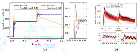
Figure 17. (a) Tracking curve for rotor speed of traditional PI controller under step change in reference speed. (b) Rotor position observation error curve of traditional PI controller under step change in reference speed.

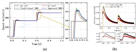
Figure 18. (a) Tracking curve for rotor speed of anti-windup ASR controller under step change in reference speed. (b) Rotor position observation error curve of anti-windup ASR controller under step change in reference speed.

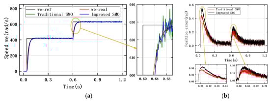
Figure 19. (a) Tracking curve for rotor speed of ISMC+IPLL controller under step change in reference speed. (b) Rotor position observation error curve of ISMC+IPLL controller under step change in reference speed.

Figure 20 gives the comparison results of the average observation error ${\Delta \omega }_e$ and ${\Delta \theta }_e$ for different controllers under the step change in reference speed. From the figure, it can be seen that the average error ${\Delta \omega }_e$ of the improved SMO for speed tracking is smaller than that of the traditional SMO in both the anti-windup ASR and ISMC+IPLL control modes, while it is higher than the traditional SMO in the PI control mode. The average observation error ${\Delta \theta }_e$ of the improved SMO for rotor position tracking is larger than the traditional SMO only in the anti-windup ASR control mode. Therefore, compared with the traditional SMO, the performance of the improved SMO is slightly optimized under the step change in reference speed.

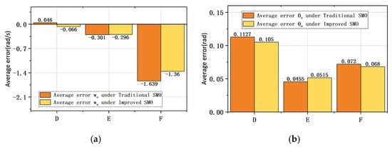
Figure 20. D-PI control. E-anti-windup ASR control. F-ISMC+IPLL control. (a) Average observation error ${\Delta \omega }_{\mathrm{e}}$ of SMO for different controllers under step change in reference speed. (b) Average observation error ${\Delta \theta }_{\mathrm{e}}$ of SMO for different controllers under step change in reference speed.

4.1.6. Hardware Implementation of PMSM Sensorless Control

To verify the observation performance of the improved SMO for ISMC+IPLL under different switching functions, a current closed-loop control with $i_d=0$ is used for the surface-mounted PMSM, and the block diagram of the system software is given in Figure 21. The detailed parameters and main control coefficients used in the experimental process are given in Table 9.

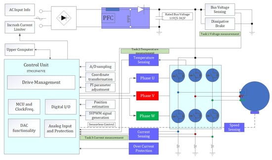
Figure 21. System block diagram of the experimental software.

Table 9. Detailed parameters and main control coefficients of PMSM used in the experiment.

Parameter	Value	Parameter	Value
Stator resistance $R_s$/Ω	0.86$\pm$ 10% ohms	Stator inductance $L_d/L_q$ (mH)	0.59 $\pm$ 20% mH
Flux linkage ${\psi }_{\mathrm{f}}$/Wb	0.1194	No. of pole pairs ${\mathrm{p}}_{\mathrm{n}}$	4
Rated speed $n_N$/rpm	3000	Rated torque $M_N$/N·m	0.6
Rated power $P$/W	62	Rated current $I_N$/A	4
Non-load current $I_P$/A	0.14	Rated voltage $U_{dc}$/V	24
Rotor inertia $J$/kg·m2	0.0027	Dead-time $T_d$/us	2
Voltage constant${ K}_e$/(V/K rpm)	4.3	SVPWM switching frequency f/KHz	20
PI controller/(kp/ki)	1/200	Current PI controller/(kp/ki)	1/40
PLL/(kp/ki)	50/600	Cut-off frequency of the LPF $f_{LPF}$/Hz	500

To address the non-ideal characteristics and errors of components in the hardware system that may degrade the accuracy and reliability of the experimental results, the following targeted measures are implemented:

Reliable hardware and software integration. The experimental platform is built by ourselves using STM32F407VE DSP microcontroller, and the executable code of the controller is generated using MATLAB/Simulink. This approach ensures consistency between the control algorithm design and hardware implementation, minimizing errors caused by manual code writing and hardware adaptation.

Inverter dead-time compensation. A dead-time is set to suppress current distortion caused by the non-ideal switching characteristics of power devices, which optimizes the accuracy of stator current sampling.

Adaptation to component parameter tolerances. Key parameters of PMSM components are clearly marked with their tolerance ranges. The adaptive sliding mode gain algorithm (Equation (17)) in the improved SMO for ISMC+IPLL is adopted to dynamically adjust the gain value, which mitigates the impact of parameter drift on the observation performance.

Current closed-loop control. A current closed-loop control strategy is employed for the surface-mounted PMSM (Figure 21). This strategy stabilizes the stator current output, reduces speed and position observation errors caused by current fluctuations, and provides a reliable current sampling foundation for the SMO of ISMC+IPLL.

High-frequency noise filtering. A low-pass filter (LPF) with a cut-off frequency is used to process the observed back-electromotive force (back-EMF) signals. This effectively filters out high-frequency noise introduced by hardware circuits, improving the signal-to-noise ratio of the observation results.

Consistent experimental variables: When testing the performance of the improved SMO under different switching functions and shaping coefficients (SC), the same SMO and phase-locked loop (PLL) circuits are used (Section 4.2). This eliminates interference caused by differences in hardware circuits, ensuring the objectivity of the comparative analysis of observation performance.

The proposed scheme is verified on the STM32F407VE-based DSP microcontroller experimental platform, as shown in Figure 22. The executable code of the controller is generated using MATLAB/Simulink to achieve sensorless control.

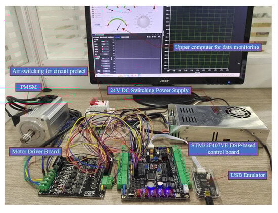
Figure 22. Experimental platform.

4.2. Comparison of Observation Performance Under Different Switching Functions and SC

In order to analyze the effect of different switching functions and SC values on the performance of the observer, the same SMO and PLL circuits are used to experimentally test the performance of the four switching functions to provide the most objective comparison results. The same level of step load is loaded on the rotor shaft during the experiment.

The initial reference speed is set to 41.8 rad/s, and the observer cannot achieve effective tracking of the rotor when the speed is below this value. The speed reaches 418 rad/s after 1.5 s. The sensorless control stage of the system is from 2 s to 8 s. The speed starts to decrease and return to the initial value at 8 s. Different types of switching functions and SC values are selected for testing, and the experimental results are presented in Figure 23, Figure 24, Figure 25, Figure 26 and Figure 27, with the same arrangement of all experimental results pictures.

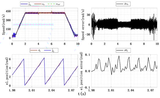
Figure 23. Experimental results of speed and position estimation under signum function.

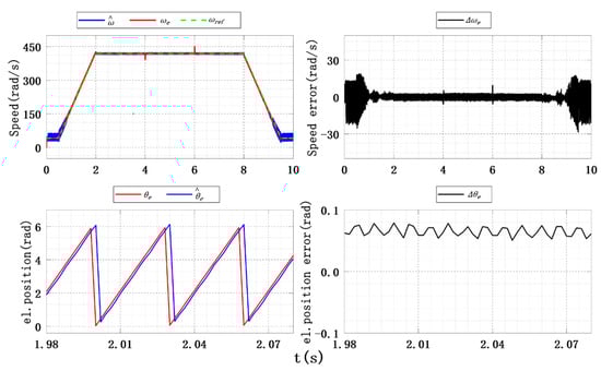
Figure 24. Experimental results of speed and position estimation under hyperbolic function, $m=0.02$.

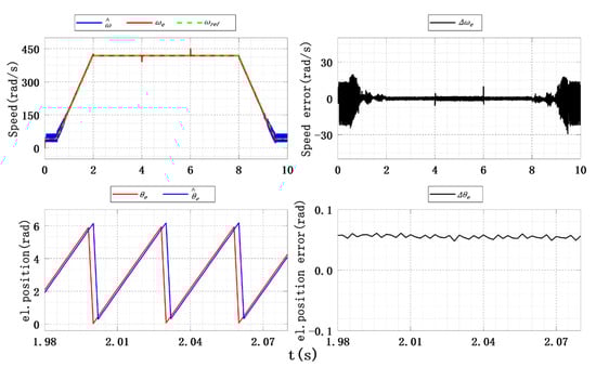
Figure 25. Experimental results of speed and position estimation under saturation function, $E_{max}=50$.

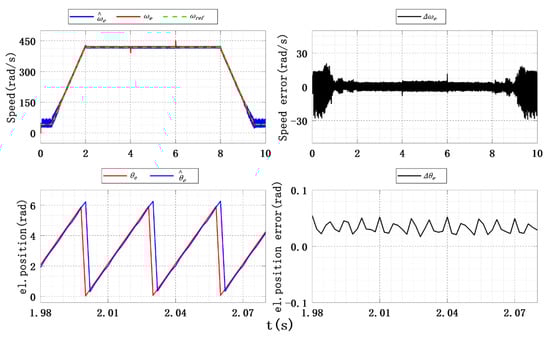
Figure 26. Experimental results of speed and position estimation under the power function, $\Delta =40$.

Figure 27. Experimental results of speed and position estimation under sigmoid function, $\alpha =0.04$.

(1)

The upper left picture shows the response curves of the actual speed and estimated speed of the improved SMO under different switching functions;

(2)

The upper right picture gives the rotor speed error $({\Delta \omega }_e={\omega }_e-{\widehat{\omega }}_e)$ curve of the improved SMO and indicates the sensorless control stage.

(3)

The bottom left picture shows a partial detail of the actual and estimated electrical angle waveforms under the sudden load.

(4)

The bottom right picture gives the waveform curve of the error $({\Delta \theta }_e={\theta }_e-{\widehat{\theta }}_e)$ when the load is suddenly added.

Figure 23 shows the experimental results of the rotor speed and position estimation under the signum function. The jitter can be observed obviously in the waveform, the speed error ${\Delta \omega }_e$ is about $\pm$38.5 rad/s at the startup, and the tracking error decreases to a certain extent during the speed increase. The average observation error in the sensorless control stage is about $\pm$15 rad/s, but the speed error decreases clearly when the load is added. The waveform of position error ${\Delta \theta }_e$ shows obvious jitter after the load is added, and the maximum tracking error reaches 0.1 rad. Therefore, the observation error of the SMO designed by using the signum function is relatively large for low speed and variable load, even in the sensor case.

The performance of the improved SMO for ISMC+IPLL using the hyperbolic function was experimented on under six different SC$\left(m\right)$ values, and the results are given in Table 10. The experimental results of the improved SMO for ISMC+IPLL designed using hyperbolic functions at $m=0.02$ are shown in Figure 24. Compared with the traditional SMO, the improved SMO for ISMC+IPLL using the hyperbolic function slightly reduced the speed error ${\Delta \omega }_{e }$ in the sensorless control stage, and effectively weakened the observed jitter. The waveform amplitude of the position tracking error ${\Delta \theta }_e$ after the load changes abruptly becomes smoother, and the maximum position tracking error is only 0.062 rad. Table 10 shows that the different shaping coefficients$m$ may make the average speed tracking error ${\Delta \omega }_e$ and the speed error jitter $\overline{{\Delta \omega }_e}$ larger again. However, the average error ${\Delta \theta }_e$ of position tracking shows a decreasing trend as the SC$\left(m\right)$ increases.

Table 10. Observation errors of speed and position measurement under different switching functions and SC.

Switching Function	SC	$\mathbf{\Delta }{\mathbf{\omega }}_{\mathbf{e}}(\mathbf{r}\mathbf{a}\mathbf{d}/\mathbf{s})$	$\overline{\mathbf{\Delta }{\mathbf{\omega }}_{\mathbf{e}}}(\mathbf{r}\mathbf{a}\mathbf{d}/\mathbf{s})$	$\mathbf{\Delta }{\mathbf{\theta }}_{\mathbf{e}}\left(\mathbf{r}\mathbf{a}\mathbf{d}\right)$	$\overline{\mathbf{\Delta }{\mathbf{\theta }}_{\mathbf{e}}}\left(\mathbf{r}\mathbf{a}\mathbf{d}\right)$
hyperbolic	$\mathrm{m}=0.004$	0.570	2.3975	0.188	0.014
hyperbolic	$\mathrm{m}=0.008$	0.693	3.446	0.121	0.02
hyperbolic	$\mathrm{m}=0.015$	0.797	3.564	0.077	0.023
hyperbolic	$\mathrm{m}=0.02$	0.636	3.526	0.062	0.0175
hyperbolic	$\mathrm{m}=0.05$	0.614	3.064	0.045	0.0165
hyperbolic	$\mathrm{m}=0.06$	0.585	2.92	0.038	0.0135
saturation	${\mathrm{E}}_{\mathrm{m}\mathrm{a}\mathrm{x}}=10$	0.78	1.6405	0.047	0.011
saturation	${\mathrm{E}}_{\mathrm{m}\mathrm{a}\mathrm{x}}=20$	0.842	1.7395	0.035	0.0105
saturation	${\mathrm{E}}_{\mathrm{m}\mathrm{a}\mathrm{x}}=35$	0.815	1.644	0.04	0.0125
saturation	${\mathrm{E}}_{\mathrm{m}\mathrm{a}\mathrm{x}}=45$	0.868	1.72	0.049	0.0115
saturation	${\mathrm{E}}_{\mathrm{m}\mathrm{a}\mathrm{x}}=50$	0.801	1.7465	0.053	0.0095
power	$\Delta =15$	0.607	3.865	0.029	0.0197
power	$\Delta =30$	0.827	5.256	0.044	0.029
power	$\Delta =40$	0.677	6.043	0.032	0.0225
power	$\Delta =50$	0.728	7.451	0.069	0.032
sigmoid	$\alpha =0.012$	0.583	3.333	0.149	0.017
sigmoid	$\alpha =0.02$	0.668	3.582	0.103	0.021
sigmoid	$\alpha =0.04$	0.647	3.371	0.063	0.0165
sigmoid	$\alpha =0.08$	0.753	2.953	0.036	0.0205
signum	—	2.106	19.599	0.048	0.0745

The observed performance of the improved SMO for ISMC+IPLL using the saturation function under five forming coefficients $E_{max}$ is shown in Table 10, and Figure 25 shows the observed results using the saturation function at $E_{max}=50$. It should be emphasized that the selection of SC value (forming coefficient) is crucial for balancing the dynamic and steady-state performance of the SMO. The traditional SMO adopts the signum function, which has fast response but extremely strong jitter. In contrast, the improved SMO for ISMC+IPLL introduces continuous switching characteristics through the SC value. When the saturation function with Eₘₐₓ = 50 is used, the jitter is reduced by 91.1% compared with the traditional signum function. Although the speed response time is slightly longer, the steady-state error is reduced by 54.6%, which fully meets the core requirement of steady-state accuracy for sensorless control of PMSM. Compared with the hyperbolic function, the speed tracking error jitter $\overline{{\Delta \omega }_e}$ using the saturation function is further weakened, while the position tracking error ${\Delta \theta }_e$ is reduced to 0.053 rad. From Figure 25, it can be seen that the observation performance of the saturation function in the sensorless control stage is better than the hyperbolic function.

The observation results of the improved SMO for ISMC+IPLL using the power function under four SC$\left(\Delta \right)$ are shown in Table 10, and Figure 26 shows the observation results using the power function at $\Delta =40$. From the figure it can be seen that, compared with the hyperbolic and saturation functions, the observation error jitter values $\overline{{\Delta \omega }_e}$, $\overline{{\Delta \theta }_e}$ of speed and position using the power function are significantly higher.

The observation results using the sigmoid function under four SC$\left(\alpha \right)$ values are shown in Table 10, and Figure 27 shows the observation results using the sigmoid function at $\alpha =0.04$. From Figure 27, it can be seen that the observation results using the sigmoid function are not very different from those using the hyperbolic function. The sigmoid function is mathematically the same as the hyperbolic function when $m=0.5\alpha$, making the speed and position tracking errors of the sigmoid and hyperbolic functions essentially equal. Therefore, the improved SMO for ISMC+IPLL can be designed using the sigmoid function instead of the hyperbolic function under certain conditions.

4.3. Analysis of Position Observation Error Under Different Switching Functions

Figure 28 gives the position observation errors of hyperbolic function at $m=0.02$, saturation function at $E_{max}=50$, power function at $\Delta =40$, and sigmoid function at $\alpha =0.04$ throughout the experimental stage, respectively. Due to the fact that the SMO adopts the same tracking strategy at low speeds, effective tracking information needs to be obtained within the sensorless control phase at 2–8 s. From the figure, it can be seen that the observation error jitter values $\overline{{\Delta \theta }_e}$ of different switching functions are not much different when the load is not added, and the observation performance of the saturation function is the best of the four types of switching functions, at only 0.0095 rad. The jitter values become larger with different switching functions after the load is added.

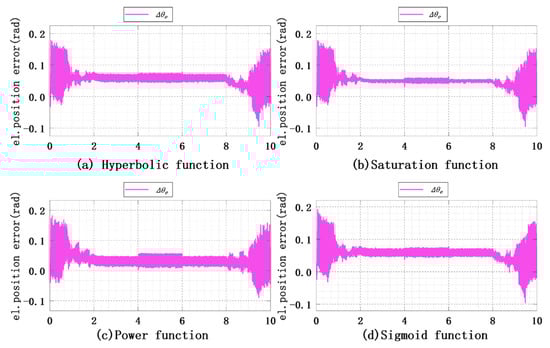
Figure 28. Experimental results for position estimation error under different switching functions.

This is mainly due to the sudden decrease in rotor speed caused by the load, resulting in a certain delay in the position compensation link in the PLL. When the load is removed, the position error jitter value returns to the previous level. The observation results of the position error are not much different because the hyperbolic function at $m=0.02$ is similar to the sigmoid function at $\alpha =0.04$ in terms of expression.

4.4. Speed Response of Different Switching Functions During Variable Load Stage

Figure 29 shows the speed response curves of different switching functions during the variable load stage at 4–6 s. The dynamic tracking performance of the observer is optimized at different levels due to the adaptive sliding mode gain used in the improved SMO for ISMC+IPLL to achieve the extraction of rotor speed and position information. The maximum speed fluctuation errors of the system under different switching functions are 2.9465 rpm, 2.7405 rpm, 2.851 rpm, and 3.071 rpm, respectively. The saturation function at $E_{max}=50$ and the power function at $\Delta =40$ suppress the jitter better than the hyperbolic function at $m=0.02$ and the sigmoid function at $\alpha =0.04$ after the load is added. The saturation function has the smallest speed error, but this does not mean that the control performance of the system is better than the other three types of switching functions when the other SC values are selected. The optimal control performance can be obtained throughout the operation stage by selecting the appropriate switching function to construct the SMO, thus improving the dynamic performance of the system.

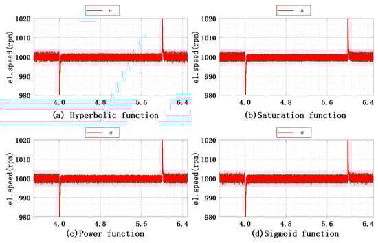
Figure 29. Experimental results for speed response under different switching functions.

5. Conclusions

(1) In this paper, a PMSM control method of ISMC+IPLL is proposed. To address the phase delay and jitter problems of the traditional SMO, the improved SMO for ISMC+IPLL is designed using the three aspects of sliding mode surface, reaching law, and switching function. The ISMC is used instead of the PI speed regulator to avoid overshoot, and can effectively suppress jitter. The system behaviors of traditional PI control, anti-windup ASR control, and the ISMC+IPLL control proposed in this paper are analyzed under load and speed variations. Considering the effects of system parameter change on control performance, different levels of external disturbances are introduced in the load and the reference speed to observe the response process under different control modes. Simulation results show that the proposed ISMC+IPLL control method has better observation performance than the other three types of controllers overall, although the dynamic response performance shows some degradation.

(2) The observation performance of the improved SMO for ISMC+IPLL based on different switching functions and SC is compared for the same SMO parameters. The results show that the improved SMO for ISMC+IPLL based on the hyperbolic function, saturation function, power function, and sigmoid function can reduce the rotor tracking error and suppress the system jitter well compared with the traditional SMO using the signum function. The tracking performance of the saturation function and the power function are optimal during the variable-load operation stage.

(3) Although the observation performance of the improved ISMC+IPLL is enhanced, the dynamic response performance needs to be further optimized, for example, by reducing the rise time and accelerating the response speed. Therefore, the new parameter optimization method needs to be proposed in subsequent work, so that the dynamic response performance can be further improved.

References

- Houari, A.; Bouabdallah, A.; Djerioui, A.; Djerioui, A.; Machmoum, M.; Auger, F.; Darkawi, A. An effective compensation technique for speed smoothness at low-speed operation of PMSM drives. IEEE Trans. Ind. Appl. 2017, 54, 647–655. [Google Scholar] [CrossRef]
- Wang, Y.R.; Xu, Y.X.; Zou, J.B. Sliding-mode sensorless control of PMSM with inverter nonlinearity compensation. IEEE Trans. Power Electron. 2019, 34, 10206–10220. [Google Scholar] [CrossRef]
- Niu, D.P.; Song, D.D. Model-based robust fault diagnosis of incipient ITSC for PMSM in elevator traction System. IEEE Trans. Instrum. Meas. 2023, 72, 3533512. [Google Scholar] [CrossRef]
- Wang, Y.O.; Zhao, M.; Huang, Y.; Jia, X.R.; Lu, M. Torque performance optimization of a novel hybrid PMSM with eccentric Halbach based on improved Taguchi method. IEEE Trans. Instrum. Meas. 2024, 73, 1–12. [Google Scholar] [CrossRef]
- Lee, Y.; Lee, S.H.; Chung, C.C. LPV H∞ Control with Disturbance Estimation for Permanent Magnet Synchronous Motors. IEEE Trans. Ind. Electron. 2017, 65, 488–497. [Google Scholar]
- Wei, Z.H.; Zhao, M.; Liu, X.M.; Lu, M. A novel variable-proportion desaturation PI control for speed regulation in sensorless PMSM drive system. Appl. Sci. 2022, 12, 9234. [Google Scholar] [CrossRef]
- Luo, B.Y.; Li, M.C.; Wang, P.; Yu, T.Y. An anti-windup algorithm for PID controller of PMSM SVPWM speed control system. In Proceedings of the 3rd International Conference on Mechatronics, Robotics and Automation, Shen Zhen, China, 20–21 April 2015; pp. 529–534. [Google Scholar]
- Lu, E.; Li, W.; Wang, S.B.; Zhang, W.G.; Luo, C.M. Disturbance rejection control for PMSM using integral sliding mode based composite nonlinear feedback control with load observer. ISA Trans. 2021, 116, 203–217. [Google Scholar] [CrossRef] [PubMed]
- Hu, J.D.; Fu, Z.Y.; Xu, R.W.; Jin, T.; Feng, Z.Y.; Wang, S. Low-complexity model predictive control for series-winding PMSM with extended voltage vectors. Electronics 2025, 14, 127. [Google Scholar] [CrossRef]
- Liu, X.D.; Zhang, Q. Robust current predictive control-based equivalent input disturbance approach for PMSM drive. Electronics 2019, 8, 1034. [Google Scholar] [CrossRef]
- Ghamri, A.; Boumaaraf, R.; Benchouia, M.T.; Mesloub, H.; Goléa, A.; Goléa, N. Comparative study of ANN DTC and conventional DTC controlled PMSM motor. Math. Comput. Simul. 2020, 167, 219–230. [Google Scholar] [CrossRef]
- Filho, C.J.V.; Xiao, D.X.; Vieira, R.P.; Emadi, A. Observers for high-speed sensorless PMSM drives: Design methods, tuning challenges and future trends. IEEE Access 2021, 9, 56397–56415. [Google Scholar] [CrossRef]
- Eker, M.; Gundogan, B. Demagnetization fault detection of permanent magnet synchronous motor with convolutional neural network. Electr. Eng. 2023, 105, 1695–1708. [Google Scholar] [CrossRef]
- Lee, K.G.; Lee, J.S.; Lee, K.B. Wide-range sensorless control for SPMSM using an improved full-order flux observer. J. Power Electron. 2015, 15, 721–729. [Google Scholar] [CrossRef]
- Wu, S.F.; Zhang, J.W.; Chai, B.B. Adaptive super-twisting sliding mode observer based robust back stepping sensorless speed control for IPMSM. ISA Trans. 2019, 92, 155–165. [Google Scholar] [CrossRef] [PubMed]
- Bao, D.Y.; Wang, H.; Wang, X.J.; Zhang, C.R. Sensorless speed control based on the improved Q-MRAS method for induction motor drives. Energies 2018, 11, 235. [Google Scholar] [CrossRef]
- Dilys, J.; Stankevič, V.; Łuksza, K. Implementation of extended Kalman filter with optimized execution time for sensorless control of a PMSM using ARM cortex-M3 microcontroller. Energies 2021, 14, 3491. [Google Scholar] [CrossRef]
- Zhao, W.X.; Jiao, S.; Chen, Q.; Xu, D.Z.; Ji, J.H. Sensorless control of a linear permanent-magnet motor based on an improved disturbance observer. IEEE Trans. Ind. Electron. 2018, 65, 9291–9300. [Google Scholar] [CrossRef]
- Ye, S. Design and performance analysis of an iterative flux sliding-mode observer for the sensorless control of PMSM drives. ISA Trans. 2019, 94, 255–264. [Google Scholar] [CrossRef] [PubMed]
- Hu, J.J.; Guo, Q.; Sun, Z.C.; Yang, D.Z. Study on low-frequency torsional vibration suppression of integrated electric drive system considering nonlinear factors. Energy 2023, 284, 129251. [Google Scholar] [CrossRef]
- Belkhier, Y.; Shaw, R.N.; Bures, M.; Islam, M.; Bajaj, M.; Albalawi, F.; Alqurashi, A.; Ghoneim, S.S.M. Robust interconnection and damping assignment energy-based control for a permanent magnet synchronous motor using high order sliding mode approach and nonlinear observer. Energy Rep. 2022, 8, 1731–1740. [Google Scholar] [CrossRef]
Disclaimer/Publisher’s Note: The statements, opinions and data contained in all publications are solely those of the individual author(s) and contributor(s) and not of MDPI and/or the editor(s). MDPI and/or the editor(s) disclaim responsibility for any injury to people or property resulting from any ideas, methods, instructions or products referred to in the content. |
© 2025 by the authors. Licensee MDPI, Basel, Switzerland. This article is an open access article distributed under the terms and conditions of the Creative Commons Attribution (CC BY) license (https://creativecommons.org/licenses/by/4.0/).