2.2.1. Multi-Branch Parallel Feature Extraction Module
In neural networks, the learning goal of each layer is to learn the mapping of the input data [
18], and when the number of network layers increases, the network becomes more difficult to train. He [
19] proposed a Residual Network (ResNet), which guides the network to learn the difference between the input data and the desired output and mitigates problems such as gradient vanishing or gradient exploding. In this paper, we apply the residual connection to the Inception module [
20], which can allow the network to pass the features of the original input directly, thus retaining more low-level feature information, which helps the transfer and fusion of multilevel features, and enhances the network’s ability to perceive features at different scales and different semantics of the image.
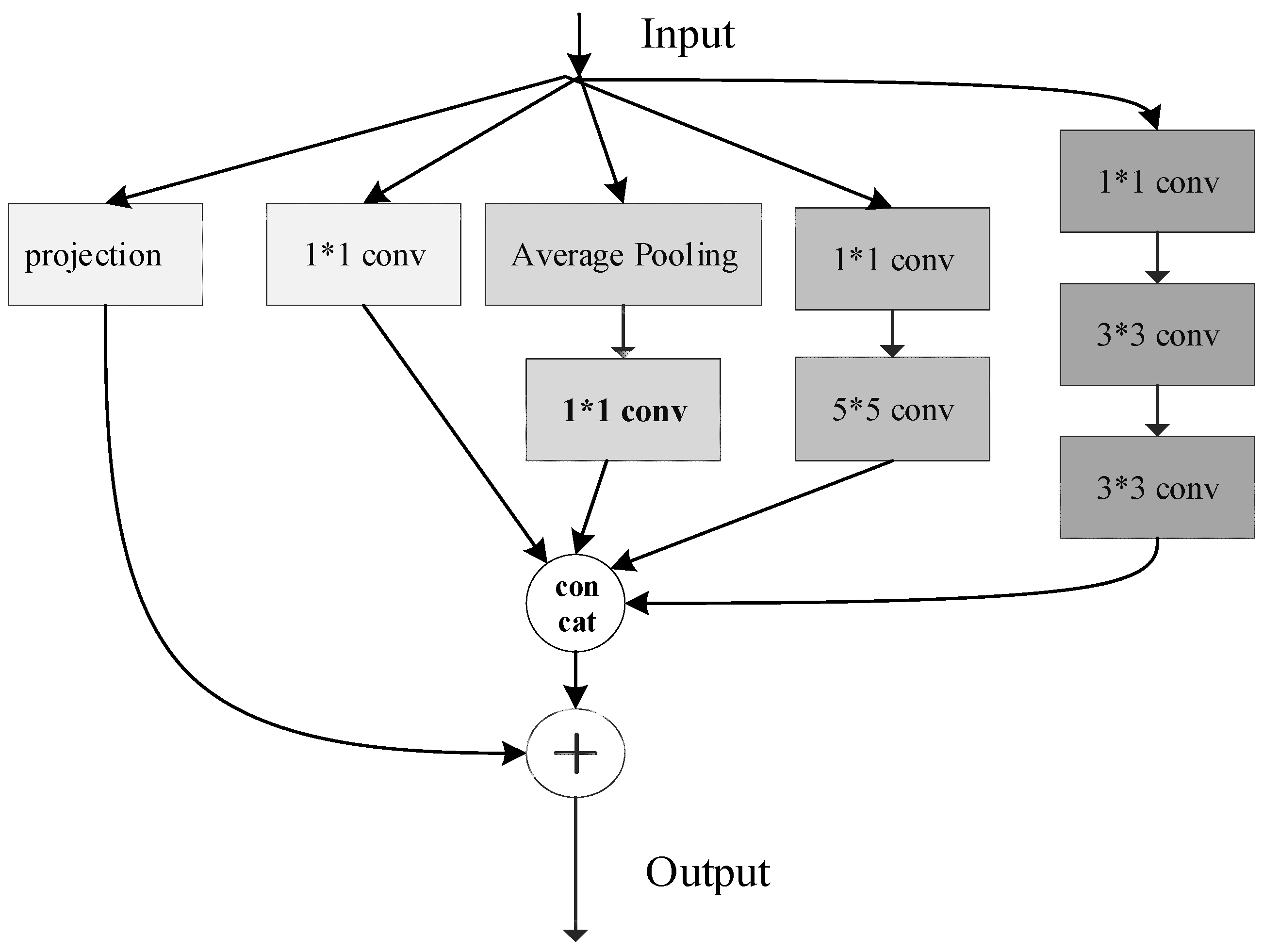
In this paper, the design of a parallel multi-branch residual feature extraction module is shown in
Figure 5. For the feature map of the upper input layer, the following four sets of convolutional branches are used for feature extraction: a convolution operation with a kernel size of 1 × 1 and a step size of 1 outputs the feature data
of the b1 channel; the output of the previous layer is average pooled and then passed through the convolutional kernel of 1 × 1, which outputs the feature data
; the output of the previous layer is feature-extracted by passing it through a convolution operation with a kernel size of 1 × 1 and a step size of 1 versus a kernel size of 5 × 5, a step size of 1, and a padding of 2. The output of the previous layer is feature-extracted, and the feature data of the b3 channel is outputted as
; the output of the previous layer is feature-extracted by passing it through a convolution operation with a kernel size of 1 × 1, a step size of 1 and a padding of 1, and a convolution operation with kernel size of 3 × 3, step size of 1, and padding of 1. The output of the previous layer is feature extracted, and the output of the b4 channel is feature data
. The output of the four sets of branches is spliced by channel as in Equation (4) to output the feature data
.
represents concatenation by channel.
The residual connection branch aligns
to the feature data
channel dimensions through the projection function
, as in Equation (5).
Finally, splice and to get the output of the current module.
2.2.2. Considering the Channel Attention Mechanism in the Frequency Domain
Appearance, texture, and color similarity between palmprint data samples is high, and small samples have local subtle differences with frequency domain information variations. The attention mechanism can enhance the model’s performance [
21] to focus on important features and suppress irrelevant information. Given that the attention mechanism is widely used in the field of computer vision, in order to capture the subtle feature changes and enhance the feature expression ability, the channel attention mechanism, which considers the frequency domain information, is introduced in the model construction, and the operation process is as follows:
Step 1. For the feature map
output from the upper layer network is divided
along the channel dimension, and for
there is
, and for each component, a Fast Fourier Transform (FFT) is applied to calculate the frequency components
, as in Equation (6).
where
are the corresponding 2D coordinates of
and
denotes the FFT basis function performed on the image.
Step 2. Combine the computed frequency domain
, as in Equation (7).
cat(.) indicates splicing along the channel.
Step 3. Construct the correlation of feature channels by fully connected layers and activation functions, and output 1 × 1 × c feature weights, as in Equation (8).
Step 4. Normalize the weights, weight (1 × 1 × c) × (H × W × c) by channel-by-channel product and output the weighted feature
, The process is shown in
Figure 6.
2.2.3. DMAML-Based Training Method for Small-Sample Learning Networks
- (1)
Weighted multi-step loss parameter update method
In the backpropagation of MAML, only the last step of the specific feature extraction network is considered for the weights [
22], while the previous multi-step updates are chosen to be optimized implicitly, leading to unstable training [
23]. In order to preserve the influence of the inner loop query set on the meta-learner parameters, an annealed weighted summation of the query set loss after the support set parameter update is performed. The parameter updating process is described in detail below in conjunction with the formula.
Step 1. Randomly obtain the task from a set of tasks in the inner loop.
Step 2. Use the support set
of the current task as the input to the small-sample palmprint feature extraction network to obtain the predicted probability
that the observation sample
belongs to the category c. Compute the cross-entropy loss
according to Equation (9).
is the sign function (take 1 if the true category of sample is equal to c, and 0 otherwise); and n denotes the number of recognized categories.
Step 3. The inner loop parameter update using the cross-entropy loss
according to Equation (10) is performed to obtain the new task-specific model parameters
under the current task.
where
denotes the loss gradient, and α is the inner loop learning rate, the initial network weight parameter
.
Step 4. Input the query set the current task into the palmprint image recognition model , and calculate the query set cross-entropy loss .
Step 5. Calculate the weight w for the current query set loss
according to Equation (11) and save
to the list.
where in m in the formula represents the current number of update steps and
represents the weight decay rate, select
as the basic annealing function, as it decreases smoothly and is commonly used in optimization algorithms; Introduce the decay rate
, adjusting the weight to
to accelerate decay adaptation for small-sample tasks.
Step 6. The process of steps 2-step to 5 above is repeated, and the task is utilized to update the inner loop parameters M times. Wherein, the process of step 5 above is a data preparation action for the inner loop phase for subsequent outer loop parameter updates, i.e., generating a multi-step loss list.
Step 7. In the MAML outer loop, step 5 of the inner loop phase is utilized to generate the multi-step loss list for updating the outer loop meta-learner model weight parameters φ by means of the optimizer RMSprop, as in Equation (12).
where φ denotes the meta-learner model weight parameter,
denotes the distribution of the set of tasks,
is the query set test loss for the parameters in a particular sub-task,
is the derivative of the loss function with respect to the parameters of the inner loop (of second order), and
is the derivative of the loss function with respect to the parameters of the outer loop model (first order), and
is the learning rate of the outer loop. In order to balance the model performance and computational efficiency, for the first
tasks, the second-order derivatives are used to solve; for the other tasks, the first-order approximate derivatives are used.
- (2)
Learning Rate Dynamic Adjustment Strategy
The outer loop learning rate of MAML determines the update speed and stability of the meta-learner parameters. When a smaller learning rate is used, the model is difficult to adapt to the changes in the training data, resulting in slower convergence of the training process and more iterative steps are required to achieve a reasonable level of performance; whereas, when a larger learning rate is used, the model is prone to overfitting on small-sample palmprint data, resulting in an unstable training process and divergence of the final model. In order to make the model converge faster and find suitable parameters stably, this paper combines progressive preheating and cosine annealing [
24,
25] to design a dynamic adjustment method for the learning rate of the outer loop. Specifically, the following steps are performed in a learning round.
Step 1. Set upper and lower bounds on the outer loop learning rate ].
Step 2. Apply Equation (13) to gradually increase the outer loop learning rate β through progressive warm-up rounds within the first learning round.
where
is the number of iterative steps of the current training,
is the total progressive warmup round iteration steps.
Step 3. Loop step 1 times to complete the learning rate warmup.
Step 4. Starting the cosine annealing phase from the current learning round, the outer loop learning rate β is dynamically updated according to Equation (14).
where
is the total number of iterative steps trained in the current learning round, and the learning rate is restarted using cosine annealing hot restart whenever all the tasks in that learning round have been performed.
The pseudocode for training DMAML is as follows Algorithm 1:
| Algorithm 1 MAML with Weighted Multi-step Loss and Dynamic Learning Rate |
Require:Task distribution Inner loop steps Learning rates Warmup steps , total steps , iteration steps
Ensure: Updated meta-parameters |
| 1: Initialize randomly. |
| 2: For each task do |
| 3: |
| 4: for to do |
| 5: Compute support loss: |
| 6: Update parameters: |
| 7: Compute query loss: |
| 8: Compute weight: |
| 9: Save to loss list |
| 10: |
| 11: end for |
| 12: Dynamic Learning Rate Adjustment: |
| 13: if then |
| 14: |
| 15: else |
| 16: |
| 17: end if |
| 18: |
| 19: if then |
| 20: Update |
| 21: else |
| 22: Update |
| 23: end if |
| 24: end for |
| 25: return |
