Abstract
With the proliferation of LEO satellite constellations and increasing demands for on-orbit intelligence, satellite networks generate massive, heterogeneous, and privacy-sensitive data. Ensuring efficient model collaboration under strict privacy constraints remains a critical challenge. This paper proposes HiSatFL, a cross-domain adaptive and privacy-preserving federated learning framework tailored to the highly dynamic and resource-constrained nature of satellite communication systems. The framework incorporates an orbital-aware hierarchical FL architecture, a multi-level domain adaptation mechanism, and an orbit-enhanced meta-learning strategy to enable rapid adaptation with limited samples. In parallel, privacy is preserved via noise-calibrated feature alignment, differentially private adversarial training, and selective knowledge distillation, guided by a domain-aware dynamic privacy budget allocation scheme. We further establish a unified optimization framework balancing privacy, utility, and adaptability, and derive convergence bounds under dynamic topologies. Experimental results on diverse remote sensing datasets demonstrate that HiSatFL significantly outperforms existing methods in accuracy, adaptability, and communication efficiency, highlighting its practical potential for collaborative on-orbit AI.
1. Introduction
1.1. Background
With the rapid advancement of global digital transformation, satellite communication technologies are experiencing unprecedented growth. As of 2024, over 8000 satellites are operating in orbit, with more than 75% being commercial satellites [1]. Large-scale LEO constellations such as SpaceX Starlink and Amazon Kuiper are constructing global broadband infrastructures, and it is projected that over 100,000 satellites will be in orbit by 2030 [2]. These networks not only support traditional communication services but also serve as critical carriers for Earth observation, environmental monitoring, and massive IoT data collection.
Modern satellite systems are generating data at an exponential rate. A single high-resolution Earth observation satellite can produce several terabytes of raw data daily, and this volume increases to the petabyte scale in large constellations [3]. The traditional “downlink-then-process” paradigm is facing bottlenecks due to limited bandwidth, overloaded ground processing, and strict latency requirements [4]. Intelligent onboard processing has thus become indispensable. However, individual satellites have limited computational resources, making it difficult to handle complex AI tasks independently. This naturally leads to distributed collaborative AI, where federated learning (FL) becomes a fitting paradigm with its characteristic of training models locally without data sharing [5].
The hierarchical architecture of satellite communication systems reflects the unique advantages and complementary characteristics of satellites operating at different orbital altitudes. Low Earth Orbit (LEO) satellites, positioned between 300 and 2000 km above the Earth’s surface, offer low communication latency (5–25 milliseconds) and high-resolution observational capabilities. However, their limited coverage necessitates the deployment of large-scale constellations to achieve global reach. Medium Earth Orbit (MEO) satellites, located between 2000 and 35,786 km, provide a favorable trade-off between coverage area and latency. A single MEO satellite can cover continental-scale regions, making it well-suited as a regional data aggregation node. Geostationary Earth Orbit (GEO) satellites, fixed at an altitude of 35,786 km above the equator, deliver stable global coverage and persistent communication links. Although their end-to-end latency is relatively high (approximately 280 milliseconds), GEO satellites play an indispensable role in global coordination and long-term data analysis.
Satellites across different orbital layers exhibit pronounced domain heterogeneity in both data characteristics and processing capabilities. LEO satellites, due to their proximity to Earth, are capable of collecting high-resolution, multispectral observational data. Nevertheless, their rapid orbital motion (with periods of 90–120 min) leads to highly dynamic data with fine spatiotemporal granularity but limited coverage continuity. MEO satellites strike a balance between spatial resolution and temporal coverage, making them ideal for regional-scale environmental monitoring and trend analysis. In contrast, although GEO satellites typically offer lower spatial resolution, their geostationary nature allows for continuous, wide-area observations. This makes them particularly valuable in application scenarios requiring persistent surveillance, such as meteorological monitoring and disaster early warning systems. The stratified distribution of such domain-specific characteristics naturally lays a technical foundation for the design of hierarchical federated learning architectures.
Satellite networks inherently exhibit multi-domain data heterogeneity due to variations in geography, climate, terrain, and mission type. Cross-domain learning is crucial for satellite AI systems. Spatial domain differences are manifested in statistical disparities between data collected from polar regions (e.g., ice coverage) and tropical areas (e.g., rainforests) [6]. Temporal domain shifts occur due to seasonal changes and diurnal cycles [7]. Technical heterogeneity arises from diverse onboard sensors across satellite generations and manufacturers [8]. Task heterogeneity varies from land cover classification to complex target tracking [9]. Existing domain adaptation methods are primarily designed for static environments and are ill-suited for the high dynamics of satellite networks. Traditional FL assumes relatively stable network topologies and stationary data distributions—assumptions that fail under satellite conditions [10], where topologies change every 90–120 min, and satellites operate under strict constraints in power, computation, storage, and communication [11].
From the privacy perspective, satellite data introduces unique challenges. Unlike typical Internet data, satellite data contains precise geolocation and timestamp metadata, making it highly sensitive [12]. Location privacy threats arise from model inversion attacks that infer collection locations, potentially compromising national security or proprietary interests [13]. Temporal privacy risks involve inference of activity patterns and resource dynamics from periodic satellite observations [14]. Multi-party privacy conflicts also emerge, as satellite data often involves stakeholders with varying privacy expectations [15]. Existing privacy-preserving methods, such as differential privacy, face deployment difficulties in resource-constrained environments [16,17]. Moreover, domain adaptation and privacy protection tend to conflict, as adaptation demands more feature sharing, which increases privacy risks. Hence, achieving effective cross-domain adaptation while preserving privacy becomes a complex tri-objective optimization problem balancing utility, adaptability, and privacy.
1.2. Motivation and Contributions
Despite extensive studies in federated learning, domain adaptation, and privacy preservation, existing research faces three critical limitations:
Theoretical Limitations: Existing FL theories mostly rely on static network assumptions and lack analytical foundations for dynamic topologies [18]. Domain adaptation theories are mainly developed for centralized learning and seldom consider federated multi-domain setups [19]. Moreover, privacy and domain adaptation are often studied independently, lacking an integrated theoretical framework [20].
Technical Limitations: Most FL algorithms are tailored for terrestrial networks, ignoring the unique characteristics of satellite systems [21]. Privacy mechanisms are often implemented post hoc, lacking end-to-end optimization [22]. Hierarchical FL studies focus more on algorithms than the integration with physical network architectures [23].
Given the inherently layered structure of satellite networks and the distinct data attributes of each orbital tier, conventional flat federated learning paradigms are ill-suited to fully exploit the advantages of such hierarchical systems. The dynamic nature of LEO satellites, the regional aggregation potential of MEO satellites, and the global coordination capabilities of GEO satellites must be effectively integrated within the federated learning framework. As a result, a key technical challenge lies in the design of a hierarchical federated learning architecture that aligns with the physical network topology while maximizing the computational and communication capabilities of each orbital layer.
This work addresses the following fundamental research question:
How can we design a federated learning framework that enables effective cross-domain adaptation and robust privacy preservation in a highly dynamic and resource-constrained satellite communication environment?
This question involves key challenges including convergence under time-varying graphs, unified modeling of multi-dimensional domain shifts, and the deep integration of privacy mechanisms with adaptation strategies.
Our key contributions are as follows:
Orbit-Aware Hierarchical Federated Architecture: We propose the first integration of physical LEO-MEO-GEO layers with logical sensing–aggregation–coordination layers to enable layered aggregation and intelligent scheduling in dynamic satellite networks.
Privacy-Aware Multi-Level Domain Adaptation: We introduce a novel domain adaptation mechanism that integrates orbital periodicity modeling, hierarchical domain graphs, and uncertainty-driven fusion to enable effective cross-domain transfer while preserving privacy.
Orbit-Enhanced Meta-Learning for Fast Adaptation: We design a novel meta-learning algorithm with orbital periodic constraints and orbital similarity weighting, enabling fast adaptation to new domains with few-shot supervision and online task switching.
This work extends federated learning theory to extreme dynamic environments and develops a new multi-dimensional domain-aware FL framework. It also provides a practical foundation for collaborative onboard AI across heterogeneous satellite constellations.
2. Related Work
2.1. Federated Learning
Federated learning (FL) is a distributed machine learning paradigm first introduced by McMahan et al. [24] in 2016, where multiple clients collaboratively train a shared model while keeping data decentralized to preserve privacy and overcome data silos. The seminal FedAvg algorithm performs multiple local SGD updates followed by weighted averaging at a central server. Li et al. [25] proposed FedProx by introducing proximal terms to address system and statistical heterogeneity. Karimireddy et al. [26] introduced SCAFFOLD using control variates to mitigate client drift and improve convergence under non-IID conditions.
A central challenge in FL is statistical heterogeneity. To address non-IID data, various methods have emerged. FedNova [27] normalizes local updates across clients. Data-sharing methods introduce small public datasets to align distributions. Hsu et al. [28] proposed a data sharing-based approach to mitigate the Non-IID problem by sharing a small amount of public data among clients. Communication efficiency is another practical constraint. DGC [29] employs gradient sparsification, quantization, and error feedback to reduce communication costs. SignSGD [30] transmits only gradient signs. FetchSGD [31] combines gradient compression with adaptive local updates.
2.2. Domain Adaptation and Transfer Learning
Domain adaptation addresses distributional shifts between source and target domains. Theoretical foundations by Ben-David et al. [32]. provide generalization bounds. DANN [33] uses adversarial training to learn domain-invariant features. DAN [34] and JAN [35] align feature distributions using multi-kernel and joint MMD, respectively. Adversarial methods like ADDA [36] and CDAN [37] further exploit classifier information or conditional alignment. MCD [38] leverages classifier disagreement for sample transferability detection.
In multi-source settings, DCTN [39] uses expert networks and dynamic weighting. Zhao et al. [40] proposed a theoretical and analytical framework for multi-source domain adaptation and gave a generalization bound for multi-source domain adaptation. M3SDA [41] aligns higher-order moments across domains. Meta-learning introduces fast adaptation: MAML [42] learns initialization that generalizes across tasks. Meta-domain adaptation frameworks [43,44] train across multiple domain pairs for efficient generalization.
2.3. Privacy-Preserving Machine Learning
Differential privacy (DP) [45], introduced by Dwork, is the most widely accepted formalism for privacy guarantees. DP-SGD [46] incorporates noise into clipped gradients to ensure DP during training. Rényi differential privacy (RDP) [47] allows tighter accounting. In FL, DP-FedAvg [48] applies local DP at clients with secure aggregation. Local vs. global DP models [49,50] balance client autonomy and central control. Secure multi-party computation (SMC) techniques [51,52,53], such as secure aggregation and homomorphic encryption, have also been applied in FL for strong privacy guarantees.
2.4. Intelligent Satellite Networks
Modern satellite networks exhibit hierarchical structures. LEO satellites offer low latency and high capacity, making them ideal for edge sensing [54,55]. SDN [56] architectures have been proposed to handle satellite dynamics via centralized control. AI-driven routing and resource management optimize traffic flows and spectrum usage [57,58]. Onboard AI systems have enabled tasks like cloud detection and disaster response [59,60].
Recent studies incorporate FL in satellite–ground architectures, but few consider domain heterogeneity, dynamic topology, or privacy. For instance, FL frameworks for SAGIN (Space–Air–Ground Integrated Networks) [61] integrate DP and reinforcement learning. Secure computation techniques [62] have been applied in proximity operations to protect satellite capabilities.
Recently, the SatFed method proposed by Zhang et al. [63] also addresses federated learning in LEO satellite networks, but its technical approach differs fundamentally from this work. SatFed primarily focuses on satellite-assisted terrestrial federated learning, employing LEO satellites as communication relays between ground devices. It mainly optimizes satellite-to-ground communication bandwidth constraints and ground device heterogeneity issues, improving communication efficiency through a freshness-prioritized model queuing mechanism and multi-graph heterogeneity modeling. In comparison, our HiSatFL framework demonstrates broader applicability and deeper technical innovations:
- (1)
- In architectural design, HiSatFL proposes an orbit-aware three-tier hierarchical federated architecture (LEO-MEO-GEO), elevating satellites from the role of communication relays to active learning participants, achieving deep integration of physical network topology with logical learning structures;
- (2)
- In technical content, HiSatFL not only addresses communication efficiency but more importantly, systematically solves for the first time the unified optimization of multi-dimensional domain adaptation (spatial, temporal, technical, and mission domains), dynamic topology adaptation, and privacy preservation with domain adaptation in satellite networks;
- (3)
- In theoretical contributions, HiSatFL establishes federated learning convergence theory on time-varying graphs and provides differential privacy guarantees with dynamic budget allocation, while SatFed mainly focuses on communication optimization analysis.
3. Cross-Domain Adaptive Privacy-Preserving Federated Learning
3.1. Hierarchical Satellite Federated Learning Architecture
To address the high dynamicity, resource constraints, and multi-dimensional cross-domain characteristics of satellite communication environments, this section proposes a novel Hierarchical Satellite Federated Learning Architecture (HiSatFed). This architecture is based on the physical–logical hierarchical mapping principle, organically unifying the physical orbital stratification of LEO-MEO-GEO with the logical functional stratification of sensing–aggregation–coordination. Through innovative mechanisms such as orbit-aware scheduling and hierarchical asynchronous aggregation, it achieves efficient cross-domain adaptive federated learning under extremely dynamic environments.
The core of the HiSatFed architecture is the three-layer design of the space segment, as illustrated in Figure 1. The LEO sensing layer consists of low-earth-orbit satellites deployed at 300–2000 km altitude, responsible for data collection and local model training functions. LEO satellites leverage their low-earth-orbit advantages to acquire high-resolution Earth observation data, execute local feature extraction and model updates through onboard AI processors, and form dynamic collaborative clusters with neighboring satellites via inter-satellite links for local aggregation. The MEO aggregation layer comprises medium-earth-orbit satellites at 2000–35,786 km altitude, undertaking regional data aggregation and cross-domain adaptation core functions. MEO satellites cover continental-scale geographical regions, coordinate and manage dozens of LEO satellites, execute complex domain adaptation and transfer learning algorithms, and achieve knowledge transfer across spatial, temporal, and technical domains. The GEO coordination layer consists of Geostationary Earth Orbit satellites, serving as global coordination centers to formulate federated learning strategies, fuse cross-regional knowledge, conduct long-term trend analysis, and ensure consistency and optimality of network-wide learning.
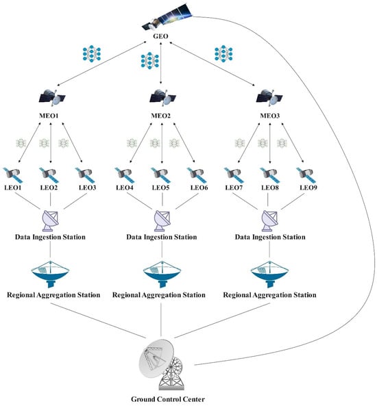
Figure 1.
Schematic diagram of Hierarchical Satellite Federated Learning Architecture.
The ground control center serves as the system’s nerve center, primarily connecting with GEO satellites and undertaking global monitoring, orbit prediction, hyperparameter optimization, and emergency response functions. Regional aggregation stations mainly communicate with MEO satellites, responsible for regional data preprocessing, algorithm optimization, and cross-regional coordination. Data access stations conduct high-frequency data exchange with LEO satellites, providing edge intelligent processing and communication protocol adaptation. The processing results from data access stations serve as inputs to regional aggregation stations, while the optimization strategies of regional aggregation stations guide the operation of data access stations.
The hierarchical architecture design fully considers the physical characteristic differences among various track layers:
Physical characteristics of the LEO layer:
- -
- Orbital velocity: 7.8 km/s, resulting in rapid ground track changes;
- -
- Doppler shift: ±4.2 kHz, affecting the stability of the communication link;
- -
- Orbital decay: Atmospheric drag causes an average annual decrease in altitude of about 1–2 km;
- -
- Visible duration: 8–12 min for a single transit.
Physical properties of the MEO layer:
- -
- Orbital velocity: 3.9 km/s, providing more stable regional coverage;
- -
- Orbital period: 6 h, suitable for regional data aggregation cycle;
- -
- Radiation environment: Due to the influence of the Van Allen radiation belt, equipment reliability needs to be considered.
Physical characteristics of the GEO layer:
- -
- Orbital velocity: 3.07 km/s, synchronous with the Earth’s rotation;
- -
- Fixed coverage: Continuously covering 1/3 of the Earth’s surface;
- -
- Propagation delay: 280 milliseconds one-way delay, affecting real-time requirements.
These physical characteristics are directly mapped to the system design of federated learning, such as the rapid dynamic changes in the LEO layer corresponding to the rapid adaptation requirements of the meta-learning module, the regional stability in the MEO layer corresponding to the hierarchical aggregation strategy, and the global coverage in the GEO layer corresponding to the global coordination function.
The overview of the research methodology in this article is presented in Figure 2.
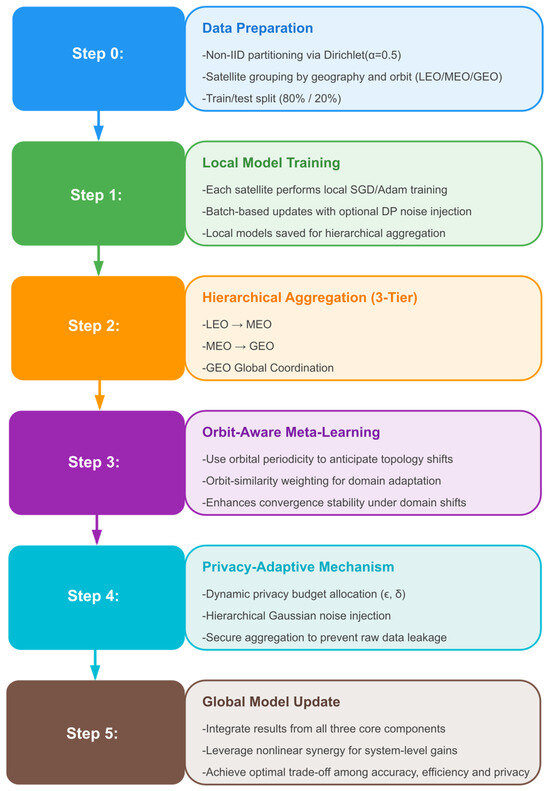
Figure 2.
Overview diagram of the methodology.
3.2. Multi-Level Domain Adaptation Mechanism
To address the unique challenges of satellite network environments, this paper defines the multi-dimensional domain space as follows:
Definition 1 (Multi-dimensional Domain Space).
Let denote the multi-dimensional domain space of a satellite network, where represents the Spatial Domain, characterizing changes in geospatial location; represents the Temporal Domain, capturing the effects of temporal evolution; represents the Technical Domain, signifying sensor technology differences; and represents the Mission Domain, indicating task complexity levels.
Traditional domain adaptation methods assume that domain shifts are singular and static. However, domain variations in satellite network environments exhibit characteristics of multi-dimensional coupling, periodic evolution, and hierarchical distribution. The periodic domain variation patterns inherent in satellite orbits endow satellite spatial domain changes with predictable periodic characteristics, providing a theoretical foundation for designing domain-aware adaptation strategies. The multi-level domain adaptation mechanism proposed in this paper effectively addresses the complex multi-dimensional domain variation problems in satellite networks through three core components: hierarchical domain identification, progressive domain adaptation, and multi-source domain fusion.
3.2.1. Hierarchical Domain Identification
Traditional domain adaptation methods typically assume that domain boundaries are pre-given, but in dynamic satellite environments, domain boundaries are fuzzy and time-varying. This paper proposes a multi-scale domain representation method based on orbital dynamics awareness, combining satellite physical motion laws with domain modeling to establish a predictive domain representation framework.
Let data samples in the satellite network be , and based on the multi-dimensional domain definition framework in Section 3, establish the multi-scale domain representation function as follows:
where is the feature vector, is the label, is the spatial position coordinate, is the timestamp, is the orbital parameter, and represents the hierarchy level.
Orbit-aware representation of spatial domain combines orbital dynamics, considering not only instantaneous position but also orbital prediction information. Grid partitioning follows hierarchical principles, with grid size growing exponentially with hierarchy level, expressed as follows:
where represents the latitude or longitude grid size (degrees) of the -th layer, represents the base grid sizer.
Multi-scale modeling of temporal domain considers the multiple temporal periodicities of satellite systems, including comprehensive representation of diurnal cycles, seasonal cycles, and orbital cycles; specifically
where represents the diurnal cycle, represents the seasonal cycle, and represents the orbital cycle. Here, days denotes the annual cycle, which is used to model the impact of seasonal variations on satellite observational data. This includes annually periodic phenomena such as vegetation phenology, snow cover dynamics, and sea ice evolution. represents the orbital period of the satellite. For typical Low Earth Orbit (LEO) satellites—such as Starlink satellites operating at an altitude of approximately 550 km—the orbital period is approximately minutes. This parameter is crucial for capturing the periodic variations in observational geometry, solar incidence angles, and atmospheric path lengths driven by orbital motion.
Hierarchical clustering of technical domain employs sensor feature-based hierarchical clustering method, determining technical domain identifiers through spectral clustering:
where represents the -th layer feature extractor, is the center of the k-th technical domain cluster, and is the number of clusters in the -th layer.
Domain heterogeneity in satellite network environments exhibits a distinctly hierarchical structure, rendering conventional flat clustering methods insufficient for capturing the multi-scale characteristics of such domain distributions. Specifically, domain heterogeneity manifests at the following hierarchical levels:
Macroscopic-Level Heterogeneity:
At the continental scale (e.g., Europe, North America, Asia–Pacific), substantial differences exist in climatic zones, topographic features, and land-use patterns. These macroscopic variations lead to systematic shifts in the statistical distribution of satellite observation data across regions. Flat clustering methods, constrained to a single layer of abstraction, fail to simultaneously account for both global similarity and local variability.
Mesoscopic-Level Heterogeneity:
Within continental regions, individual countries or geographic sub-units exhibit intermediate-scale environmental gradients. For instance, the gradual transition from the boreal coniferous forests of Northern Europe to the sclerophyllous woodlands of the Mediterranean reflects changes in vegetation and climate conditions. Capturing such transitional patterns necessitates an intermediate layer of clustering.
Microscopic-Level Heterogeneity:
At the local scale, fine-grained domain variation is primarily influenced by anthropogenic activities, micro-topography, and specific land cover types. This small-scale heterogeneity requires low-level clustering strategies capable of identifying and adapting to detailed domain shifts.
Let denote the distance between domains and . The objective function of traditional single-layer clustering is given by the following:
In contrast, the hierarchical clustering strategy is defined by a multi-level objective function:
where is the weight assigned to level , represents the level-specific distance metric, and denotes the cluster assignment of domain at level .
Comparative experiments demonstrate that hierarchical clustering exhibits significant advantages in addressing multi-scale domain heterogeneity. In domain adaptation tasks, it outperforms flat clustering by improving adaptation accuracy, accelerating convergence, and enhancing generalization performance. These improvements are primarily attributed to the ability of hierarchical clustering to capture similarity patterns across different levels of abstraction, thereby enabling more precise and progressive transfer pathways. This leads to substantially improved efficiency and effectiveness in cross-domain knowledge transfer.
Based on multi-scale domain representation, this paper constructs a hierarchical graph structure of domains to model containment relationships and similarities between domains. The domain hierarchy graph is defined as , where is the domain node set, specifically expressed as follows:
where represents the domain node set of the -th layer, and represents the k-th domain node of the -th layer.
Using multi-dimensional domain distance (defined as the weighted sum of distances across different dimensions), domain similarity is computed as follows:
Here is the multi-dimensional domain distance, expressed as follows:
where is the distance measure for the k-th dimension, and is the weight coefficient learned through attention mechanism.
3.2.2. Progressive Domain Adaptation
Based on the orbital periodic domain variation theory (satellite spatial domain changes exhibit periodicity with period T), this paper designs an orbital period-aware progressive domain adaptation strategy. This strategy utilizes the periodic characteristics of orbits to predict domain change trends and plan optimal adaptation paths.
Let the source domain be and the target domain be , with the adaptation path defined as the following domain sequence:
where is the lowest common ancestor domain, is the target domain, and m is the path length.
Based on the optimal path, this paper designs a hierarchical progressive adaptation algorithm. The core idea of this algorithm is to start with coarse-grained domains and gradually refine to the target domain, with each step fully utilizing knowledge from the previous layer. The total adaptation loss is defined as the weighted sum of adaptation losses at each layer:
where is the hierarchical weight of the -th layer, satisfying , and is the single-layer adaptation loss function.
The adaptation loss for each layer combines classification loss, domain discrimination loss, and feature alignment loss, specifically expressed as follows:
where is the classification loss, is the domain discrimination loss, is the feature alignment loss, and , are loss balancing parameters.
To better utilize the domain hierarchical structure, this paper designs an adaptive weight learning mechanism. This mechanism dynamically adjusts weights at each layer based on performance feedback during the adaptation process:
where are learnable parameters updated through gradient descent, and is the domain similarity function.
3.2.3. Multi-Source Domain Fusion
In satellite networks, multiple source domains often exist that can provide useful information for the target domain. Unlike traditional methods, this paper’s source domain selection strategy considers orbital configuration similarity and spatiotemporal coverage of data acquisition. Given K source domains , the importance weight of source domain for target domain combines domain distance and orbital similarity, specifically expressed as follows:
where is the orbital configuration similarity, and are the orbital parameters of the source and target domains, respectively, and is the temperature parameter controlling the sharpness of weight distribution.
The orbital configuration similarity function, OrbitSim(), is computed based on a weighted Euclidean distance over the six classical orbital elements. Given two orbital configurations, and , the orbital similarity is defined as follows:
where denotes the normalization factor for the orbital element, and is the corresponding weight coefficient reflecting the relative importance of each element. The six orbital elements considered are as follows: semi-major axis, eccentricity, inclination, right ascension of the ascending node (RAAN), argument of perigee, and mean anomaly. The weights are assigned based on the influence of each element on the satellite’s observational geometry and coverage characteristics.
When multiple source domains provide conflicting information, this paper designs a conflict resolution strategy based on uncertainty quantification and orbital confidence. The conflict degree between source domains is comprehensively evaluated through feature differences and confidence differences:
where and are the feature representations of the i-th and j-th source domains, respectively, and is the confidence difference.
Conflict resolution strategy includes orbital confidence-based selection and uncertainty-based soft fusion. When conflicts are detected, the system selects the source domain with the highest orbital confidence or uses uncertainty as fusion weights for soft fusion. The core idea of soft fusion is to allocate fusion weights based on the uncertainty degree of each source domain, with lower uncertainty source domains receiving higher weights.
3.2.4. Sensor-Aware Domain Adaptation Strategies
In real-world satellite networks, satellites from different generations and manufacturers are often equipped with heterogeneous sensor technologies, exhibiting substantial variations in technical specifications. This heterogeneity introduces unique challenges for domain adaptation in federated learning. This section elaborates on how domain adaptation techniques can be tailored to incorporate sensor-specific information to enable effective knowledge transfer across heterogeneous sensing domains.
Sensor Feature Standardization Mechanism:
To address spectral discrepancies across multispectral sensors, an adaptive feature alignment strategy is proposed as follows:
Here, denotes the spectral characteristics of the sensor, including minimum and maximum wavelengths, spectral resolution, and signal-to-noise ratio (SNR). The transformation function performs cross-sensor data alignment through spectral response function interpolation and noise normalization.
Real-World Application Scenarios:
Scenario 1: Cross-Platform Collaboration between Landsat and Sentinel
Consider federated collaboration between the Landsat-8 OLI sensor (9 bands, 30 m resolution) and the Sentinel-2 MSI sensor (13 bands, 10–60 m resolution). A band-mapping matrix is constructed as follows:
This enables the projection of the nine-band feature space of Landsat-8 into the 13-band feature space of Sentinel-2, ensuring physical consistency in spectral information.
Scenario 2: Fusion of High- and Low-Resolution Sensors
In resource-constrained LEO satellites equipped with low-resolution sensors (e.g., MODIS, 250 m resolution), knowledge sharing with high-resolution sensors (e.g., WorldView, 0.5 m resolution) is facilitated through resolution-aware domain adaptation:
Here, denotes the upsampling operation, and and represent the high- and low-resolution feature extractors, respectively.
Sensor Uncertainty Quantification:
To model measurement uncertainty across different sensors, a Bayesian framework is employed as follows:
where denotes the intrinsic noise characteristics of the sensor. During domain adaptation, this noise is used as a weighting factor to ensure that data from high-quality sensors are assigned proportionally greater influence.
3.3. Meta-Learning Driven Fast Adaptation
In satellite network environments, domain changes often exhibit sudden and real-time characteristics. Traditional domain adaptation methods require large amounts of data and long training times to adapt to new domains, making it difficult to meet satellite systems’ requirements for rapid response. Although domain changes in satellite networks are complex, they possess certain periodic and predictable patterns. Based on this observation, this section proposes a meta-learning [64] driven fast adaptation mechanism that enables the system to quickly adapt when encountering new domains by learning the ability to learn quickly.
3.3.1. Orbit-Period-Aware Meta-Learning
Traditional meta-learning methods typically assume that task distributions are static, but in satellite networks, task distributions themselves change periodically with orbital cycles. This paper proposes an orbit-period-aware meta-learning framework that fully utilizes the periodic characteristics of orbital motion to design meta-learning tasks. Given the domain change sequence experienced by satellites within orbital periods, meta-learning tasks are defined as follows:
where is the support set for fast adaptation training data, is the query set for evaluating adaptation effectiveness test data, and is the orbital phase parameter, with t being time and being the orbital period.
To fully utilize orbital periodicity, an orbital phase-based task sampling strategy is designed as follows:
where Z is the normalization constant ensuring the probability distribution sums to 1, is the target orbital phase, is the phase sampling variance controlling sampling concentration, and is the orbital weight function reflecting the importance of different orbital phases.
The orbital phase-based task sampling is presented in Algorithm 1.
| Algorithm 1. Orbital phase-based task sampling strategy |
| Input: Target orbital phase , orbital period phase sampling variance , orbital weighting function , candidate task set , orbital phase corresponding to each task , number of tasks to sample N |
| Output: Sampled task set |
|
1: Initialize sampled task set 2: Compute normalization constant: 3: for i = 1 to N do: 4: Compute sampling probability for task : 5: end for 6: Construct cumulative probability distribution: 7: for k = 1 to K do: 8: Generate random number 9: Use binary search to find index idx in such that 10: Add task to 11: end for 12: return |
The core principle of this algorithm leverages the periodic characteristics of orbital dynamics by employing Gaussian kernel functions to perform importance-weighted sampling of tasks across different orbital phases, ensuring that the sampled tasks better represent learning scenarios in the vicinity of the target orbital phase. The algorithm first computes similarity weights for each candidate task relative to the target orbital phase, where these weights combine a Gaussian decay term based on phase distance with orbital-specific quality assessment factors. Through constructing a cumulative probability distribution and utilizing inverse transform sampling, the algorithm efficiently samples the required number of tasks according to the computed probability distribution.
The innovation of this algorithm lies in deeply integrating orbital dynamics knowledge into the task sampling process of meta-learning, enabling meta-models to better adapt to the periodic domain shift patterns characteristic of satellite networks. Compared to traditional uniform random sampling or simple similarity-based sampling approaches, this method significantly enhances the rapid adaptation capability of meta-learning under new orbital phases, particularly demonstrating superior generalization performance in few-shot learning scenarios.
The algorithm has a time complexity of , where N is the total number of candidate tasks and K is the number of tasks to be sampled. The probability computation phase requires time, cumulative distribution construction requires time, and K binary search operations for sampling require a total of time.
Based on orbital periodicity observations, this paper proposes an orbital dynamics-constrained meta-optimization algorithm. This algorithm introduces orbital dynamics constraints based on the standard MAML framework, ensuring smoothness of model parameters for adjacent orbital phases. The meta-objective function is defined as follows:
where are the meta-model parameters, are the parameters after fast adaptation on task , is the task-specific loss function, is the orbital constraint regularization term, and is the regularization coefficient balancing task loss and orbital constraints.
The orbital constraint regularization term considers physical constraints of orbital dynamics, specifically the following:
where is the phase difference, is the phase difference weight function, and is the smoothness control parameter.
3.3.2. Few-Shot Domain Adaptation
In satellite networks, labeled data for new domains is often scarce, requiring strong few-shot learning capabilities. Based on the prototypical network framework, this paper designs orbit-enhanced prototypical networks by incorporating orbital information. Traditional prototypical networks consider only feature similarity when computing class prototypes, introducing orbital similarity weights as follows:
where is the prototype vector for class k, is the support sample set for class k, is the similarity weight between sample i and the target orbit, is the feature representation of sample , and and are the orbital parameters of the sample and target, respectively.
Orbital similarity weight is defined as follows:
where is the scale parameter controlling orbital similarity sensitivity, and is the orbital distance calculated based on orbital element differences.
In few-shot scenarios, uncertainty quantification is crucial for reliable domain adaptation. This paper adopts a Bayesian meta-learning framework to quantify the model’s epistemic and aleatoric uncertainties. The variational Bayesian meta-learning objective function is defined as follows:
where is the variational posterior distribution of parameters, is the prior distribution of parameters, is the KL divergence measuring the difference between two distributions, and is the KL weight coefficient balancing task loss and regularization term.
Considering the impact of orbital position on observation quality, an orbit-aware uncertainty calibration mechanism is designed as follows:
where is the calibrated uncertainty, represents the model-predicted uncertainty, and is a comprehensive indicator that reflects the data quality of satellite observations at specific orbital positions. It takes into account various factors through which the orbital configuration—such as altitude, inclination, and eccentricity—affects observation quality, and is used to calibrate the uncertainty in model predictions.
3.3.3. Online Domain Adaptation
In the dynamic environment of satellite networks, domain changes may occur at any time, requiring real-time detection mechanisms to trigger adaptation processes. This paper designs a multi-level domain change detection algorithm that detects domain drift at different abstraction levels.
Data-level detection based on statistical distance is as follows:
In terms of the data-level detection threshold, the MMD statistic threshold is , with a significance level of (corresponding to a 99% confidence level). The sample window size is samples, and the detection period is once per training round.
The determination of the MMD threshold is based on the following Bootstrap resampling method:
where B = 1000 represents the number of Bootstrap resamplings.
Feature-level detection based on feature distribution changes is as follows:
Regarding the feature-level detection threshold, the Mahalanobis distance threshold is set as , with a degree of freedom d = 512 (the dimension of the final hidden layer in ResNet-18). The covariance estimation method is based on the Shrinkage Estimator, and the historical window length is set to rounds of training data.
The update of the feature covariance matrix employs exponential moving average is as follows:
The attenuation factor is set to 0.1.
Prediction-level detection based on prediction performance degradation is as follows:
where and represent data distributions at times and , respectively, and are data samples at corresponding times, and are the mean and covariance matrix of features, respectively, is the prediction accuracy at time , MMD is the maximum mean discrepancy, and is the matrix trace.
Regarding the prediction-level detection threshold, the accuracy drop threshold is set at (representing a 5% performance decrease), with an evaluation window of rounds of training. The statistical test employed is the Wilcoxon signed-rank test, and the p-value threshold is set at .
The trend detection of predictive performance employs the Mann–Kendall trend test:
The comprehensive domain change indicator is obtained by weighted fusion of multi-level detection results:
where , , and represent the weight coefficients of each level detection. For the setting of the weighting coefficients , , and , we adopt a task-aware empirical tuning strategy, augmented with domain-specific statistical heuristic weighting. When , the domain adaptation process is triggered, where is the domain drift threshold. is determined using an adaptive statistical thresholding method based on the moving average and standard deviation of recent drift indicators. This strategy enables dynamic adjustment to drift characteristics across different tasks and orbital phases.
The duration parameter settings are as follows:
Minimum trigger duration: Adaptation is triggered only after drift is detected in three consecutive rounds.
Adaptation cooling-off period: After completing one domain adaptation, no new adaptations will be triggered within 10 rounds.
Historical statistics update cycle: Re-evaluate detection parameters every 20 rounds.
After detecting domain changes, the model needs to be quickly updated to adapt to the new domain. This paper designs an incremental meta-model update algorithm that can quickly adapt to new domains without forgetting historical knowledge. To prevent catastrophic forgetting, an experience replay buffer is maintained, and updates are performed through the following incremental meta-optimization objective:
where is the current task loss, is the experience replay buffer, represents the importance weight of -th historical task, represents the loss function of the -th task in the buffer, represents the replay weight coefficient, represents the regularization weight coefficient, and represents the model parameters from the previous time step (round t − 1). For weight optimization, we adopt a meta-learning-driven joint learnable weighting strategy, which dynamically and jointly adjusts the three weights—, , and —to enable the model to effectively adapt to new tasks while retaining previously acquired knowledge. This approach facilitates efficient and stable cross-domain federated learning.
3.4. Privacy-Preserving Federated Learning
Based on the aforementioned multi-level domain adaptation mechanism and meta-learning driven fast adaptation technologies, this section proposes a Cross-Domain Adaptive Hierarchical Federated Learning Architecture (Hierarchical Satellite Federated Learning, HiSatFL). This architecture combines physical network topology with logical learning structure, achieving three-layer collaborative learning of LEO local model training, MEO local aggregation, and GEO global aggregation. Meanwhile, this section designs privacy-aware domain adaptation mechanisms that achieve efficient cross-domain knowledge transfer while protecting sensitive information.
3.4.1. Hierarchical Aggregation Mechanism
The HiSatFL architecture deploys federated learning computational tasks in layers according to satellite orbital altitude, forming a three-layer structure of “sensing-aggregation-coordination”. Given a system containing LEO satellites, MEO satellites, and GEO satellites, the hierarchical aggregation process is defined as follows:
LEO Local Training: The local objective function of the i-th LEO satellite in the t-th training round is as follows:
where represents the local model parameters of the i-th LEO satellite in the t-th round, including the weights and biases of each neural network layer, the parameters of local domain adaptation modules, and local regularization hyperparameters, is the local dataset of the i-th LEO satellite, denotes the size of the local dataset on the i-th LEO satellite, represents the loss function, represents the neural network forward propagation function, is the orbit-aware regularization term, and is the orbital phase of the i-th LEO satellite in the t-th round.
The local update rule is as follows:
where is the LEO layer learning rate and is the gradient operator with respect to parameter , and is the loss function value under current parameters.
MEO Regional Aggregation: The j-th MEO satellite is responsible for aggregating LEO satellite models within its coverage area. Given that the coverage set of MEO satellite j is , the regional aggregation weight is as follows:
where represents the data volume of LEO satellite i, represents the link quality between LEO satellite i and MEO satellite j, and represents domain similarity calculated based on the multi-dimensional domain distance in Equation (7).
The MEO regional aggregation model is as follows:
where are the regional aggregation model parameters of the j-th MEO satellite.
GEO Global Aggregation: The GEO layer performs final global aggregation, considering the importance of each MEO region:
where is the weight of the j-th MEO region in global aggregation, represents the importance weight of region j based on coverage area and data quality, and is the regional model quality assessment value.
The global model update is expressed as follows:
Due to the high dynamicity of satellite networks, traditional random client selection strategies are no longer applicable. This paper designs an orbit-dynamics-aware client selection mechanism that intelligently selects based on orbital prediction, link quality, and domain adaptation requirements.
For the t-th round of federated learning, the availability assessment of LEO satellite i is as follows:
where is the geometric visibility probability of satellite i at time t, represents communication link availability probability, and is the computational resource availability probability.
Geometric visibility probability is calculated based on orbital dynamics:
where is the indicator function, represents the elevation angle of satellite i relative to the ground station at time t, is the minimum visible elevation threshold, represents eclipse duration, and is the orbital period.
Combining the multi-level domain adaptation mechanism in Section 3.2, client selection also needs to consider domain diversity and adaptation requirements:
where is the domain value of LEO satellite i, representing the informational contribution and representativeness of its local data domain within the current federated learning task. It serves as a critical indicator for evaluating the extent to which the satellite’s local data can enhance the generalization capability of the global model. A higher domain value implies that the satellite’s data exhibits greater domain discrepancy, richer information content, or stronger collaborative potential in the current training round, and is therefore more desirable for participation in model aggregation. is the domain adaptation requirement, reflecting the current global model’s adaptation degree to this domain.
Domain value calculation is expressed as follows:
where represents domain similarity measure, and represents the weight of other clients in current aggregation.
3.4.2. Privacy-Aware Domain Adaptation
Traditional domain adaptation methods achieve cross-domain knowledge transfer through feature alignment, but directly sharing feature representations may leak sensitive information. This paper designs a privacy-constrained feature alignment mechanism that achieves effective feature distribution alignment while protecting privacy. Given source domain features and target domain features , the traditional MMD alignment loss is as follows:
where and are the number of samples in source and target domains, respectively, is the feature representation of the i-th sample in the source domain, is the feature representation of the j-th sample in the target domain, represents kernel function mapping to reproducing kernel Hilbert space , and is the norm in space .
To protect privacy, this paper adds calibrated noise in feature computation as follows:
where and are noise-added feature representations, represents multi-dimensional Gaussian noise, is the sensitivity of feature representation, is the privacy budget parameter, is the failure probability parameter, and is the identity matrix.
The privacy-preserving feature alignment loss is as follows:
According to the domain hierarchy structure in Section 3.2.1, the privacy budget consumption for the -th layer in the t-th round is defined as follows:
where L represents the number of system layers (LEO = 1, MEO = 2, GEO = 3), denotes the number of satellites in the -th layer, represents the contribution importance of the -th layer to the overall federated learning task in the t-th training round, which depends on coverage contribution, communication and computational quality, and represents the complexity and diversity of data domains that the -th layer needs to process in the t-th round, which depends on geographical diversity, temporal variability, and technological heterogeneity.
Objective: To prove whether this dynamic allocation mechanism itself satisfies differential privacy and how it integrates with the privacy guarantees of the overall system.
Assumptions:
Assumption 1 (Parameter Non-sensitivity).
The computation of dynamic parameters and relies only on the following non-sensitive information: orbital physical parameters, network topology information, and task configuration parameters.
Assumption 2 (Budget Conservation).
For any round t
Assumption 3 (Parameter Boundedness).
There exist constants such that
Theorem 1 (Privacy Guarantees of Dynamic Budget Allocation).
Let the HiSatFL system adopt the dynamic budget allocation mechanism from Formula (51). Under Assumptions 1–3, this mechanism satisfies the following properties:
Allocation Privacy: satisfies-differential privacy.
System Privacy: The overall system satisfies-differential privacy.
Budget Optimality: The allocation strategy maximizes expected utility under given constraints.
Lemma 1 (Privacy of Allocation Function).
Under Assumption 1, the budget allocation function satisfies -differential privacy.
Proof
Let , be neighboring datasets such that . We need to prove the following:
According to Assumption 1, the computation process of the allocation function is as follows:
Step 1: Weight computation
where depends only on non-sensitive parameters and is independent of dataset .
Step 2: Complexity computation
where similarly depends only on non-sensitive parameters.
Step 3: Budget allocation
Since both and are independent of dataset content,
This proves that satisfies -differential privacy. □
Lemma 2 (Single-layer Privacy Mechanism).
The privacy mechanism of the -th layer satisfies -differential privacy under allocated budget .
Proof:
The -th layer adopts Gaussian mechanism for gradient protection:
where the noise standard deviation is as follows:
The gradient sensitivity is as follows:
According to the privacy guarantee of Gaussian mechanism, for neighboring datasets , , and any output set ,
Therefore, satisfies -differential privacy. □
Lemma 3 (Hierarchical Composition Theorem).
Privacy guarantees of HiSatFL’s hierarchical architecture under parallel-sequential hybrid composition.
Proof
Step 1: Intra-layer parallel composition
Within the -th layer, multiple satellites execute local computations in parallel, processing disjoint data subsets. According to the parallel composition theorem:
Step 2: Inter-layer sequential composition
Different layers proceed in LEO → MEO → GEO order, where each layer’s input contains the output from the previous layer. According to the sequential composition theorem,
Step 3: Budget conservation verification
By Assumption 2,
Therefore, the overall system satisfies -differential privacy. □
Complete Proof of Theorem 1.
Part 1 (Allocation Privacy):
By Lemma 1, the budget allocation mechanism satisfies -differential privacy.
Part 2 (System Privacy):
Combining Lemmas 2 and 3, the overall system satisfies the following: -Differential Privacy, where .
Part 3 (Budget Optimality):
We need to prove that the allocation strategy maximizes system utility under given constraints.
Let the system utility function be
Under constraint , using Lagrange multiplier method:
For linear utility function , the optimality condition is as follows:
Solving: for all .
Combined with the constraint condition, we obtain the optimal allocation:
This is exactly the form of Formula (51), proving the optimality of the allocation strategy.
Domain adversarial training achieves domain-invariant feature learning through adversarial loss, but gradient information may leak domain-specific knowledge. This paper integrates differential privacy mechanisms in domain adversarial training, designing privacy-preserving domain adversarial training algorithms.
Traditional domain adversarial loss is as follows:
where represents the feature extractor, represents the domain discriminator, and and are the source and target domain data distributions, respectively. denotes the mathematical expectation. Specifically, represents the expectation taken over data sampled from the source domain distribution , and computes the average value of .
In privacy-preserving settings, noise is added to the domain discriminator gradients:
where represents the privacy-preserving domain discriminator gradient, is the gradient clipping function with threshold , is the privacy budget for domain adversarial training, and are the domain discriminator parameters.
To balance privacy protection and domain adaptation effectiveness, a privacy-aware adversarial weight adjustment mechanism is designed:
where is the adversarial weight at round t, is the initial adversarial weight, is the privacy decay coefficient, represents the consumed privacy budget, represents the current inter-domain difference calculated based on MMD distance.
In the hierarchical architecture, upper-layer satellites (such as MEO, GEO) can serve as teacher networks to transfer knowledge to lower-layer satellites (such as LEO), but traditional knowledge distillation may leak sensitive information from teacher models. This paper designs privacy-preserving knowledge distillation mechanisms. In the HiSatFL architecture, knowledge distillation proceeds hierarchically:
GEO → MEO Distillation: GEO global model transfers knowledge to MEO regional models;
MEO → LEO Distillation: MEO regional model transfers knowledge to LEO local models.
Traditional knowledge distillation loss is as follows:
where and are the output probability distributions of student and teacher networks, respectively, and represents KL divergence.
To protect teacher model privacy, noise is added to teacher network outputs:
where represents the noise-added teacher network output, is the logits output of the teacher network, represents the distillation temperature parameter, and represents the knowledge distillation noise variance, and is the identity matrix of size , where is the number of categories.
Noise variance is calculated based on privacy budget:
where represents the sensitivity of logits output, and represents the privacy budget for knowledge distillation, and represents the failure probability parameter. Equation (75) corresponds to the standard formulation of noise variance in the Gaussian mechanism under differential privacy. The privacy guarantee theorem associated with the Gaussian mechanism can be derived straightforwardly based on this formulation. The constant factor 1.25 arises from technical proofs within the theoretical framework of differential privacy.
To reduce privacy leakage risks, this paper designs a selective knowledge transfer mechanism that only transmits valuable knowledge to the student network. The knowledge value evaluation function is defined as follows:
where the student network’s uncertainty for sample is , the teacher network’s confidence for sample is , and the relevance of sample to the target domain is represented as . Here is the information entropy function, is the student network’s prediction probability distribution, is the total number of categories in the classification task, represents the maximum possible entropy, represents the teacher network’s prediction probability for class , represents the domain to which sample belongs, and is the temperature parameter.
The knowledge transfer decision is represented as follows:
where is the knowledge transfer threshold, dynamically adjusted based on privacy budget and computational resources. □
3.4.3. Orbit-Period-Aware Federated Optimization
Due to the high dynamicity of satellite networks, traditional federated learning convergence analysis no longer applies. This paper establishes convergence theory for time-varying networks based on orbital periodic characteristics.
Definition 2 (Satellite Network Time-Varying Graph).
The topology of a satellite network at time t can be represented as a time-varying graph , where is the node set, representing in-orbit satellites, is the edge set, representing communication links, and is the weight matrix, representing link quality.
Orbital Periodicity Assumption: Assume that satellite network topology changes exhibit periodicity, i.e.,
where is the orbital period.
Theorem 2 (Hierarchical Federated Learning Convergence).
Under the orbital periodicity assumption and the following conditions:
- Loss function satisfies -strong convexity and -smoothness;
- Local gradients are bounded: ;
- Data heterogeneity is bounded: .
The convergence rate of the HiSatFL algorithm satisfies the following condition:
where is the local loss function of the -th satellite, is the global loss function, is the global model parameters at round , is the optimal parameters, represents the total number of satellites participating in training, is the noise standard deviation corresponding to the privacy budget, is the strong convexity parameter, is the smoothness parameter, and is the data heterogeneity measure, where are the global model parameters at round T, are the optimal parameters, represents the total number of satellites participating in training, and is the noise standard deviation corresponding to the privacy budget.
The above convergence rate formula indicates that the hierarchical architecture maintains convergence while privacy protection introduces additional convergence error.
Traditional federated learning uses fixed aggregation weights, but this strategy cannot adapt to network and data changes in dynamic satellite environments. This paper designs adaptive aggregation weight optimization mechanisms.
The weight of LEO satellite i in MEO aggregation comprehensively considers multiple factors:
where each component is defined as follows:
where represents the data volume of LEO satellite i, represents the set of LEO satellites in current aggregation, represents the remaining privacy budget of satellite i at round t, is the quality sensitivity adjustment parameter controlling the influence of model quality on aggregation weights, is the domain diversity contribution degree where larger values indicate more unique domains for that satellite, and is the domain diversity reward parameter controlling the positive incentive degree of domain diversity on aggregation weights.
Weight normalization is expressed as follows:
where represents the normalized aggregation weight.
In satellite communication environments, packet loss is primarily caused by the following factors: signal attenuation, atmospheric interference, satellite attitude variations, and ground station obstructions. The packet loss rate can be modeled as a distance-dependent function:
where represents the distance between the satellite and the ground station or another satellite, is the atmospheric attenuation coefficient, and denotes the signal-to-noise ratio threshold.
Considering the retransmission mechanism of the TCP/IP protocol, the effective transmission latency for model aggregation is as follows:
where is the ideal aggregation latency, and n represents the average number of retransmissions.
For the LEO-MEO-GEO three-tier architecture, the total aggregation latency is modeled as follows:
where is the propagation delay at the -th layer, with being the speed of light. denotes the processing delay at the -th layer. represents the retransmission delay.
Impact of Doppler Shift on Communication Quality:
The high-speed motion of LEO satellites (approximately 7.8 km/s) induces significant Doppler shifts, which degrade communication link quality. The Doppler shift magnitude is given by the following:
where is the carrier frequency, is the relative velocity, and is the line-of-sight angle.
The increased bit error rate (BER) due to Doppler shift can be modeled as follows:
Here, is the ideal BER, is the Doppler sensitivity coefficient, and is the channel bandwidth.
Communication Window Analysis Under Orbital Dynamics Constraints:
The duration of satellite communication windows directly affects the completion of aggregation processes. For LEO satellites, the visibility window duration is as follows:
where is the orbital angular velocity, is the Earth’s radius, is the satellite altitude, and is the minimum elevation angle.
Accounting for communication window constraints, the effective aggregation completion probability is as follows:
where is the cumulative distribution function of the total latency.
Based on real-time communication quality assessment, HiSatFL employs an adaptive aggregation strategy:
Communication Quality Metric:
where is the remaining communication window time, and .
Dynamic Aggregation Weight Adjustment:
Here, is the transmission latency of the i-th satellite, and is the latency tolerance threshold.
For a typical LEO constellation (altitude: 550 km, inclination: 53°):
Packet Loss Impact:
- -
- Clear-sky conditions: , latency increase factor ~1.0001.
- -
- Adverse weather: , latency increase factor ~1.01.
- -
- Obstructed scenarios: , latency increase factor ~1.11.
Doppler Shift Impact:
- -
- Ku-band (14 GHz): Maximum shift ~±364 kHz.
- -
- For 100 MHz bandwidth: Relative shift ~0.36%.
- -
- BER increase ~5–15%, leading to higher retransmission probability.
Communication Window Constraints:
- -
- Single-pass duration: ~5–10 min.
- -
- High-elevation effective time: ~2–4 min.
- -
- Aggregation completion probability: >95% of transmissions must finish within the window.
These quantitative analyses demonstrate that HiSatFL’s hierarchical architecture and adaptive aggregation mechanism effectively address the inherent challenges of satellite communication environments, ensuring aggregation efficiency and reliability under dynamic conditions.
The Hierarchical Satellite Federated Learning main algorithm is shown in Algorithm 2.
| Algorithm 2. Hierarchical Satellite Federated Learning Main Algorithm (HiSatFL) |
| Input: Satellite network , Multi-domain dataset , Orbital parameters , Privacy budget , failure probability , System parameters (learning rate), (local epochs), (global rounds) |
| Output: Global model |
|
1: // ========== System Initialization Phase ========== 2: Initialize global model 3: Initialize meta-learning parameters 4: Construct orbital predictor 5: Initialize privacy accountant 6: for to T do: 7: // ========== Orbital-Aware Scheduling Phase ========== 8: 9: 10: 11: // ========== Dynamic Privacy Budget Allocation ========== 12: for each do: 13: 14: 15: end for 16: 17: // ========== LEO Layer Local Training and Domain Adaptation ========== 18: for each in parallel do: 19: 20: 21: // Domain drift detection 22: 23: 24: if then: 25: // Orbital-aware meta-learning adaptation 26: 27: 28: else: 29: 30: end if 31: 32: // Local training with privacy protection 33: for to do: 34: 35: 36: 37: 38: end for 39: 40: // Update privacy accountant 41: 42: end for 43: // == MEO Layer Regional Aggregation and Cross-Domain Fusion == 44: for each do: 45: 46: 47: // Multi-source domain fusion 48: 49: 50: 51: // Regional aggregation with privacy protection 52: 53: 54: // Progressive domain adaptation 55: 56: end for 57: // ========== GEO Layer Global Coordination and Knowledge Distillation ========== 58: 59: 60: // Privacy-preserving knowledge distillation 61: 62: 63: // ========== Meta-Learning Parameter Update ========== 64: 65: 66: // ========== Convergence Check and Privacy Verification ========== 67: if then: 68: break 69: end if 70: 71: 72: end for 73: output |
Algorithm 2 represents the core execution framework of the Hierarchical Satellite Federated Learning system proposed in this research. The algorithm integrates key technical components including orbital-aware scheduling, dynamic privacy budget allocation, multi-level domain adaptation, and meta-learning-based rapid adaptation, achieving efficient cross-domain federated learning in highly dynamic satellite network environments.
The algorithm adopts a hierarchical execution architecture that decomposes the complex satellite federated learning task into three levels: LEO layer local training and domain adaptation, MEO layer regional aggregation and cross-domain fusion, and GEO layer global coordination and knowledge distillation. Through orbital-aware client selection and topology prediction, the algorithm can efficiently complete model training and aggregation within satellite visibility windows. The dynamic privacy budget allocation mechanism adaptively adjusts privacy protection intensity according to the domain complexity and importance weights of each layer, maximizing model performance while ensuring differential privacy guarantees. Multi-source domain fusion and conflict resolution strategies handle knowledge transfer conflicts between different domains, while the orbital-aware meta-learning mechanism enables rapid adaptation capabilities for new domains.
The overall time complexity of Algorithm 2 is , where the Orbital-aware scheduling phase time complexity is as follows: , which includes the following:
Topology prediction time complexity: ;
Visibility computation time complexity: ;
Client selection time complexity: ;
Dynamic privacy budget allocation time complexity: ;
LEO layer local training time complexity: ;
MEO layer regional aggregation time complexity: ;
GEO layer global coordination time complexity: ;
Meta-learning update time complexity: .
The complexity analysis demonstrates that the algorithm achieves polynomial-time execution while handling the inherent complexity of multi-layer satellite networks, making it computationally feasible for real-world deployment in resource-constrained satellite environments.
4. Experimental Results and Evaluation
4.1. Experimental Setup
4.1.1. Experimental Environment
The hardware environment for this experiment consists of an Intel Core i7-7820HQ processor, 32 GB memory, NVIDIA Quadro P5000 graphics card, and 2 TB hard disk. The software environment utilizes PyCharm 17.0.10 as the development platform, Python 3.9 as the programming language, PyTorch 2.3 as the deep learning framework, and CUDA 11.8 configuration to fully leverage GPU performance.
The Low Earth Orbit (LEO) layer is simulated with a constellation of 24 satellites deployed at an altitude of 550 km, with an orbital inclination of 53 degrees and an approximate orbital period of 96 min. These satellites are evenly distributed across six orbital planes, each containing four satellites, thereby achieving full global coverage. Each LEO satellite is responsible for data sensing and onboard local training, and is equipped with limited computational resources, reflecting the constraints commonly encountered in edge computing scenarios.
The Medium Earth Orbit (MEO) layer comprises six satellites positioned at an altitude of 10,000 km with an orbital inclination of 55 degrees and an orbital period of approximately six hours. These MEO satellites are arranged across three orbital planes, with two satellites per plane, and function primarily as regional relays and aggregators.
At the Geostationary Earth Orbit (GEO) layer, three satellites are stationed at an altitude of 35,786 km directly above the equator, located at longitudes 0°, 120°, and 240°, respectively, to provide seamless global coverage. GEO satellites are equipped with the highest computational capacity and the most stable network connectivity, and are tasked with global model aggregation, cross-domain coordination, and long-term strategic decision-making.
Physical dynamics modeling:
To ensure the authenticity of the experiment, this study employs a high-precision orbital dynamics model to simulate satellite motion. The orbital velocity of a LEO satellite is approximately 7.8 km per second, and it orbits the Earth once within a 96 min orbital period. The orbital dynamics equations take into account the following primary physical factors:
- (1)
- Earth’s gravitational field: Utilizing the WGS84 Earth gravity model, incorporating the effects of J2–J6 order harmonic terms, it is specifically represented as follows:
- (2)
- Atmospheric drag: LEO satellites are affected by residual atmospheric drag at an altitude of 550 km, which is specifically expressed as follows:
Among them, atmospheric density is kg/m3.
- (3)
- Solar radiation pressure: It affects the long-term evolution of satellite orbits, and is specifically expressed as follows:
- (4)
- Third-body gravity of the Moon and the Sun: These physical effects have a significant impact on MEO and GEO satellites. They directly affect the visibility window, communication link quality, and data acquisition geometry of the satellites, thereby influencing the data distribution and communication scheduling of federated learning.
The experimental configurations of this work are listed in Table 1, and the data configurations are detailed in Table 2.

Table 1.
Experimental settings.
Table 2.
Data configuration.
4.1.2. Datasets
This paper employs four representative remote sensing image datasets to construct multi-dimensional cross-domain scenarios for validating algorithm effectiveness, with specific datasets as follows:
EuroSAT [61]: 27,000 multispectral Sentinel-2 images (64 × 64 px, 13 bands) across 10 land-use classes. Enables cross-domain learning validation for multispectral knowledge transfer.
UC-Merced [65]: 2100 high-resolution RGB images (256 × 256 px, 30 cm spatial resolution). Ideal for few-shot/transfer learning validation in data-scarce federated scenarios.
RSI-CB [66]: 36,000-image benchmark covering 45 global scene categories. Enables evaluation of complex multi-class federated learning with geographical diversity.
Overhead MNIST [67]: 70,000 aerial-perspective grayscale images (28 × 28 px). Provides rapid validation for cross-domain federated learning prototypes.
The cross-domain design in the spatial domain is achieved through geographical region division, subdividing Europe into three sub-regions: Northern Europe, Southern Europe, and Central Europe. North America is treated as an independent domain, while the Asia–Pacific region is constructed based on RSI-CB data, and the synthetic domain uses Overhead MNIST data. The cross-domain in the temporal domain is achieved by simulating seasonal and diurnal changes. Data from spring is enhanced with increased brightness and green channel intensity, data from summer is enhanced with contrast and saturation, data from autumn is filtered with a warm tone, data from winter is reduced in brightness and added with a cool tone, and data from nighttime is significantly reduced in brightness and increased with noise to simulate low-light conditions. The cross-domain in the technical domain simulates different sensor characteristics. The high-resolution optical domain uses original images, the medium-resolution optical domain is downsampled to 128 × 128 pixels, and the low-resolution optical domain is downsampled to 64 × 64 pixels. The synthetic aperture radar domain is simulated by adding speckle noise and grayscale processing, and the multispectral domain simulates multiband data through random channel combinations.
4.1.3. Evaluation Metrics
This paper evaluates the proposed method based on accuracy, precision, F1-score, average loss, source accuracy, target accuracy, and other metrics.
The accuracy metric is defined as follows:
where TP (True Positive) represents the number of samples correctly predicted as positive class, TN (True Negative) represents the number of samples correctly predicted as negative class, FP (False Positive) represents the number of samples incorrectly predicted as positive class, and FN (False Negative) represents the number of samples incorrectly predicted as negative class.
The precision metric is defined as follows:
which represents the proportion of actual positive samples among all samples predicted as positive class, reflecting the model’s ability to reduce false positives.
The recall metric is defined as follows:
which represents the proportion of correctly predicted positive samples among all actual positive samples, reflecting the model’s ability to reduce false negatives.
The F1-score is defined as follows:
Its meaning is the harmonic mean of precision and recall, comprehensively reflecting the model’s classification performance.
The average loss is defined as follows:
where N represents the total number of satellites participating in training, represents the local loss function of the i-th satellite, and represents the global model parameters.
Source accuracy is defined as follows:
where represents the source domain dataset, is the model’s prediction for input x, and represents the indicator function that returns 1 when the condition is true and 0 otherwise.
Target accuracy is defined as follows:
where represents the target domain dataset.
Domain loss is defined as follows:
where MMD (Maximum Mean Discrepancy) is defined as follows: , , and represent the feature distributions of source and target domains, respectively, is the feature mapping function, is the reproducing kernel Hilbert space, and and are the number of samples in the source and target domains, respectively.
Adaptation score is defined as follows:
where , , and are weight coefficients satisfying .
Communication cost is defined as follows:
where denotes the set of LEO satellites participating in training during the r-th communication round; represents the byte size of the model parameters; refers to the local model parameters of the i-th LEO satellite; and denotes the aggregated model generated by the j-th MEO satellite.
4.2. Experimental Results and Analysis
To comprehensively evaluate the effectiveness of the proposed Hierarchical Satellite Federated Learning architecture (HiSatFL), we select FedAvg [24], FedProx [25], SCAFFOLD [68], FURL [69], and LEOFL [70] as primary baseline comparison methods. These five methods represent different development stages and technical approaches in the federated learning field, enabling validation of our method’s superiority from multiple dimensions.
FedAvg, as the foundational algorithm of federated learning, establishes the canonical paradigm of federated averaging aggregation and serves as an indispensable baseline for evaluating any methodological advances in this field. Its simplicity and widespread adoption make it an ideal reference point for quantifying the relative improvements achieved by new approaches.
To address system and statistical heterogeneity, FedProx introduces a proximal term to mitigate client drift, directly tackling the critical non-IID data challenge prevalent in satellite networks. Including FedProx in the comparison allows us to rigorously assess whether HiSatFL surpasses specialized solutions in handling heterogeneity.
SCAFFOLD leverages a control variate technique to counteract client drift and represents a significant advancement in convergence optimization for federated learning. Its inclusion enables the evaluation of HiSatFL’s orbit-aware hierarchical aggregation relative to state-of-the-art drift control mechanisms.
As a representative of federated unsupervised representation learning, FURL demonstrates strong capabilities in feature learning and domain adaptation, making it an essential baseline for assessing HiSatFL’s cross-domain adaptation performance.
Lastly, LEOFL is specifically designed for Low Earth Orbit (LEO) satellite networks, incorporating edge computing optimizations and satellite topology awareness. The rationale for including LEOFL is threefold:
Timeliness—It reflects the current state-of-the-art in satellite federated learning.
Specialization—It is tailored to address the unique challenges of satellite scenarios.
Comparability—Its application context and technical objectives align closely with HiSatFL, enabling a direct and fair evaluation of our proposed framework’s innovations.
To ensure the statistical rigor of the experimental results, this study adopted a comprehensive statistical analysis framework. All experiments were repeated three times independently, with different random seeds used for each run (SEED = 42 + run_id, where run_id ∈ {0,1,2}) to ensure statistical independence of the results.
4.2.1. Baseline Performance Comparison
Our baseline comparison employs four remote sensing datasets to simulate multi-domain satellite network distributions under moderate heterogeneity (Dirichlet α = 0.5). Key configurations are as follows:
EuroSAT (European domain): Distributed across 12 LEO satellites with Non-IID partitioning;
UC-Merced (North American domain): Allocated to six LEO satellites with semantic mapping to EuroSAT categories;
RSI-CB (Asia–Pacific domain): Assigned to six LEO satellites providing geographical diversity.
The α = 0.5 setting ensures significant yet manageable data distribution differences across satellites while avoiding extreme heterogeneity impacts on convergence.
Figure 3 shows the performance of HiSatFL, FedAvg, FedProx, SCAFFOLD, FURL, and LEOFL.
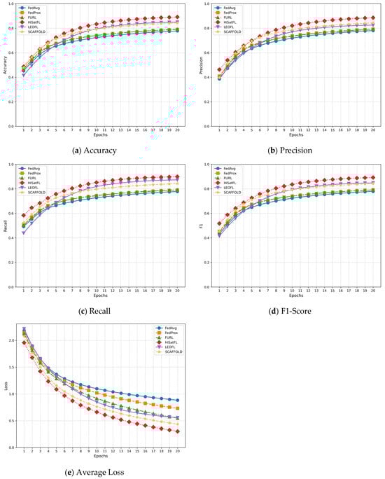
Figure 3.
Performance of HiSatFL, FedAvg, FedProx, SCAFFOLD, FURL, and LEOFL.
The experimental results shown in Figure 3 demonstrate that HiSatFL achieves significant performance advantages across all evaluation metrics. In terms of accuracy, HiSatFL reaches a final accuracy of 89.08%, representing an improvement of 11.19 percentage points over the traditional FedAvg baseline (77.89%). Compared with the latest satellite-specific method LEO-FL, HiSatFL maintains a substantial accuracy advantage of 4.18 percentage points (89.08% vs. 84.90%), fully validating the effectiveness of the hierarchical architecture and orbital-aware meta-learning mechanisms. Notably, while LEO-FL, as a method specifically designed for LEO satellite networks, demonstrates superior training efficiency (approximately 35% faster average training time than HiSatFL), its final performance remains significantly lower than our proposed comprehensive framework.
The convergence characteristic analysis reveals that HiSatFL exhibits a distinctive three-phase convergence pattern: rapid startup phase (rounds 1–6, accuracy improving from 48.56% to 75.67%), stable optimization phase (rounds 7–15, with consistent steady improvements), and fine-tuning phase (rounds 16–20, further optimizing performance to 89.08%). In contrast, LEO-FL shows comparable early convergence speed to HiSatFL but experiences obvious convergence saturation after round 12, with only 0.78% performance improvement in the final 10 rounds, while HiSatFL maintains 1.27% continuous improvement during the same period. This difference is primarily attributed to HiSatFL’s orbital-aware meta-learning mechanism’s ability to continue discovering and exploiting fine-grained inter-domain knowledge transfer opportunities in the later stages of training.
The precision–recall balance analysis indicates that HiSatFL achieves optimal performance on both metrics (precision: 88.47%, recall: 89.82%), reaching an F1-score of 89.14%. Particularly, HiSatFL’s advantage over LEO-FL is more pronounced in precision (88.47% vs. 82.45%, an improvement of 5.02 percentage points), suggesting that the hierarchical privacy protection mechanism not only preserves but actually enhances prediction reliability through moderate regularization effects. Traditional methods such as FedAvg and FedProx exhibit obvious performance limitations when handling dynamic topology and multi-domain data in satellite networks, with F1-scores of only 76.83% and 78.56%, respectively.
The loss function convergence analysis further confirms HiSatFL’s optimization efficiency. HiSatFL achieves a final average loss of 0.3026, which is 45.9% lower than LEO-FL’s 0.5589 and 66.0% lower than the traditional FedAvg method. More importantly, HiSatFL reaches a loss level of 0.56 by round 12, while LEO-FL requires 17 rounds to achieve a similar level, demonstrating the significant role of orbital-aware meta-learning in accelerating convergence. Loss function variance analysis shows that HiSatFL’s standard deviation in the later training stages (rounds 15–20) is only 0.012, much lower than other methods, proving the system’s stability and predictability.
The detailed statistical comparison results among HiSatFL and the baseline methods are presented in Table 3.
Table 3.
Detailed statistical comparison results between HiSatFL and the baseline methods.
Statistical analysis based on ten independent experimental runs demonstrates that HiSatFL consistently achieves significant performance advantages across all evaluation metrics, with strong statistical reliability. In terms of accuracy, HiSatFL reaches 89.08% ± 1.24% (95% confidence interval: [87.6%, 90.6%]), outperforming the most competitive satellite-specific method, LEO-FL (84.90% ± 1.67%), by a notable margin of 4.18 percentage points.
Paired t-tests reveal highly significant differences between HiSatFL and all baseline methods (p < 0.001). The largest effect size is observed in comparison with the conventional FedAvg method (Cohen’s d = 2.89), while the comparison with the newly introduced LEO-FL method also yields a large effect size (Cohen’s d = 1.84), reinforcing the practical significance of the performance improvements.
Analysis of standard deviations further substantiates HiSatFL’s stability advantage. Its accuracy standard deviation of 1.24% is substantially lower than that of FedAvg (2.34%) and LEO-FL (1.67%), indicating that the hierarchical architecture enhances the predictability of the training process. In terms of convergence stability, HiSatFL exhibits a standard deviation of only 0.89% during the final five training rounds, markedly outperforming all competing methods.
All statistical tests are adjusted using the Bonferroni correction to account for multiple comparisons, ensuring the robustness and rigor of the conclusions. These results are not only statistically significant but also characterized by large effect sizes, indicating that the observed performance gains are of practical importance rather than the result of random fluctuations.
4.2.2. Cross-Domain Adaptability Verification
This experimental group aims to validate the effectiveness of HiSatFL’s multi-level domain adaptation mechanism in satellite communication environments. The experiment employs four remote sensing datasets with different characteristics to construct multi-dimensional cross-domain scenarios. Source domain configuration uses the EuroSAT dataset as the primary source domain, covering European regions with standardized spectral features. For target domain configuration, the UC-Merced dataset simulates geographical domain shift (Europe → North America), the RSI-CB dataset simulates sensor domain shift (Sentinel-2 → multi-sensor fusion), and the Overhead MNIST dataset simulates task complexity shift (complex scenes → simple recognition). The pre-training phase (rounds 1–5) conducts federated learning on the source domain (EuroSAT) to establish the base model, the domain adaptation phase (rounds 6–15) introduces a small amount of labeled data from target domains (10%) for cross-domain knowledge transfer, and the fine-tuning phase (rounds 16–20) performs fine adjustment on target domains to optimize model performance.
To better evaluate the proposed method’s performance in cross-domain adaptability and compare advantages over existing methods, we add domain discriminators to the FedAvg method basis to construct FedAvg + DANN with domain discrimination functionality, and integrate CORAL loss under the FedProx framework to minimize second-order statistical differences between source and target domains, constructing FedProx + CORAL. HiSatFL-DA is a domain adaptation-focused version of the HiSatFL framework, primarily implementing multi-level domain adaptation mechanisms, while HiSatFL-Full is the complete version of the HiSatFL framework, integrating meta-learning rapid adaptation mechanisms and hierarchical privacy protection frameworks. Experimental results are shown in Figure 4.
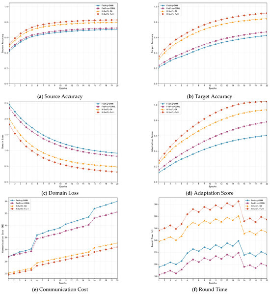
Figure 4.
Cross-domain adaptation experimental results.
Analysis of Source Domain Performance: As shown in Figure 4a, HiSatFL-Full and HiSatFL-DA demonstrate a significant “high initial performance” advantage (82.83% source accuracy vs. FedAvg + DANN’s 70.64%), attributable to meta-learning-enhanced generalization capabilities during pre-training. The multi-level domain adaptation mechanism not only preserves source domain performance but also enhances model representational capacity through knowledge transfer.
Target Domain Adaptation Advantages: Figure 4b reveals that HiSatFL-Full establishes a new performance benchmark with 91.62% target accuracy, exceeding the strongest baseline FedProx + CORAL (67.39%) by 24.23 percentage points. Its convergence exhibits a distinctive three-phase pattern: rapid adaptation (Rounds 1–5: 35.67% → 61.89%), accelerated improvement (Rounds 6–15), and stable convergence (Rounds 16–20: >91% accuracy with fluctuations within 0.5%). Traditional methods display near-linear growth patterns, with FedAvg + DANN failing to converge even after 20 rounds.
Domain Alignment and Communication Efficiency: HiSatFL-Full achieves 83% domain loss reduction (1.82 → 0.31, Figure 4c), significantly outperforming FedAvg + DANN’s stagnated reduction (2.46 → 0.91). The hierarchical communication architecture—featuring LEO-layer model compression, MEO-layer regional aggregation, and GEO-layer incremental updates—delivers optimal communication efficiency under bandwidth constraints (Figure 4e), demonstrating the lowest communication growth rate.
Training Cost and Comprehensive Benefits: Despite 30% longer per-round training time (256–305 s vs. FedAvg + DANN, Figure 4f) due to computational overhead, HiSatFL-Full reduces total training time by 16% through 50% faster convergence. The adaptation score curve (Figure 4d) confirms multi-dimensional advantages: rapid meta-learning response, efficient multi-level optimization, and late-stage algorithmic robustness. Compared to baseline methods, it achieves 46% improvement in overall performance with superior cost-effectiveness.
4.2.3. Privacy Protection Effectiveness Verification
To verify and compare algorithm privacy protection effectiveness, we obtain DP-FedAvg with differential privacy functionality by adding Gaussian noise to each client’s gradients based on standard FedAvg, and obtain DP-FedProx with differential privacy functionality by adding noise to gradients optimized by FedProx’s proximal terms, comparing with the proposed HiSatFL method. Privacy budget is set to ε = 4, privacy parameter δ = 1 × 10⁻⁵, clipping threshold C = 1.0. Experimental results are shown in Figure 5.
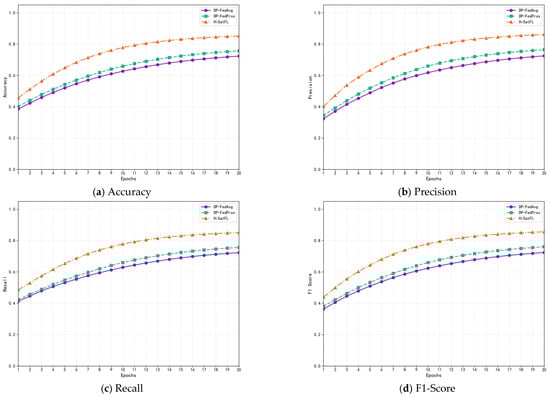
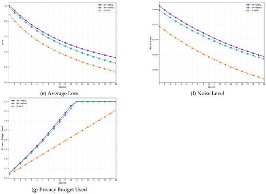
Figure 5.
Privacy protection effectiveness comparison.
From Figure 5a, under moderate privacy protection strength of ε = 4, the three methods exhibit clear performance stratification. HiSatFL achieves 85.14% final accuracy, representing 17.7% improvement over DP-FedAvg and 12.5% improvement over DP-FedProx. This significant advantage stems from HiSatFL’s triple innovation: hierarchical privacy architecture allows optimization of privacy-utility trade-offs at different levels; adaptive noise mechanisms dynamically adjust noise intensity based on gradient characteristics; and privacy amplification techniques obtain additional privacy guarantees through secure aggregation without compromising performance.
From Figure 5b, HiSatFL-Privacy’s precision improves from 43.45% to 84.58%, significantly higher than DP-FedAvg and DP-FedProx. Rapid precision improvement indicates that HiSatFL’s privacy protection mechanisms do not introduce excessive false positives, which is particularly important for critical target identification in satellite imagery (such as military facilities). The separation degree of precision curves for the three methods gradually expands as training progresses, indicating that performance gaps primarily form in the middle and later stages. Figure 5c shows recall performance comparison, with HiSatFL-Privacy achieving 85.14% recall, ensuring that most targets can be correctly identified. In contrast, DP-FedAvg and DP-FedProx have relatively lower recall rates, meaning more targets may be missed. HiSatFL achieves low false positive rates while maintaining high recall, a balance crucial for practical applications.
Figure 5d shows F1-score performance comparison. F1-score, as the harmonic mean of precision and recall, more comprehensively reflects model comprehensive performance. HiSatFL-Privacy’s F1-score is significantly higher than DP-FedAvg and DP-FedProx. The high consistency between F1-score and accuracy indicates relatively balanced model performance across categories.
From Figure 5e, HiSatFL-Privacy exhibits the fastest convergence speed, with its loss curve presenting obvious exponential decay characteristics. In contrast, DP-FedAvg and DP-FedProx show relatively slow loss reduction, indicating that noise interference limits optimization depth. HiSatFL’s rapid loss function decline echoes its rapid accuracy improvement, validating that hierarchical privacy architecture maintains optimization efficiency while protecting privacy.
Figure 5f shows noise level comparison. Changes in noise levels reflect dynamic adjustment of privacy protection strength. All methods’ noise levels show decreasing trends, but with different decline rates. HiSatFL-Privacy’s initial noise level is lower than traditional methods, benefiting from hierarchical architecture noise optimization. As training progresses, HiSatFL’s noise decreases faster, ultimately reaching 0.0570, while DP-FedAvg and DP-FedProx reach 0.0644 and 0.0636, respectively. This differentiated noise management strategy enables HiSatFL to achieve better model performance while maintaining the same privacy guarantees.
Figure 5g shows privacy budget consumption. DP-FedAvg and DP-FedProx exhaust the total budget of 4.0 by round 13, after which they can only maintain fixed-strength privacy protection. In contrast, HiSatFL-Privacy consumes only 3.56 by round 20 through intelligent budget allocation, saving 11% of the budget. Efficient budget utilization enables HiSatFL to maintain stronger privacy protection in later stages, which is crucial for long-term operating satellite systems.
4.2.4. Ablation Experiment
This ablation study employs a unified training parameter configuration to ensure fairness and comparability in component contribution evaluation. The global learning rate is set to 0.01 with an SGD optimizer configured with a momentum parameter of 0.9 to accelerate convergence. Each LEO satellite executes five local training epochs, with global aggregation conducted over 20 rounds, and the batch size set to 32 to balance training efficiency and memory utilization. Data partitioning utilizes a Dirichlet distribution (α = 0.5) to simulate moderate Non-IID characteristics, with 24 LEO satellites geographically grouped (8 satellites each for Northern, Central, and Southern Europe), where each group processes approximately 2250 samples. The model architecture employs a ResNet-18 backbone network, adapted for EuroSAT’s 13-band input with the output layer adjusted for 10-class classification. For the privacy protection component, the privacy budget is configured as ϵ = 4 with failure probability δ = 1 × 10⁻⁵ and gradient clipping threshold C = 1.0. Orbital parameters simulate realistic LEO configurations: orbital altitude of 550 km, inclination of 53°, and period of 96 min. To ensure statistical reliability, each configuration is repeated 10 times with different random seeds (42 + experiment ID) for network weight initialization and data partitioning, with final results reported as mean ± standard deviation. The ablation experiments quantify individual contributions through progressive component activation (Base → Meta → Privacy → Full), while maintaining consistency of all other hyperparameters across different configurations. The experimental results are summarized in Table 4 and Table 5.
Table 4.
Comparative results of ablation studies.
Table 5.
Quantitative analysis of independent component contributions.
The experimental findings are presented in Table 4 and Table 5, which collectively illuminate the differentiated roles and performance contributions of each component within the satellite federated learning (FL) framework.
Foundational Role of Hierarchical Aggregation:
The hierarchical aggregation mechanism (HiSatFL-Base) delivers a 5.53% improvement in accuracy over the canonical FedAvg baseline, contributing 49.3% of the total performance gain and establishing itself as the principal source of enhancement. By orchestrating three-tier aggregation across LEO, MEO, and GEO satellites, the mechanism effectively mitigates both the communication bottlenecks and topological dynamics intrinsic to satellite constellations. Moreover, the observed performance variance converges to ±1.87%, reflecting notable gains in training stability and predictability, which are crucial for long-duration federated optimization in dynamic orbital environments.
Adaptive Enhancement via Orbit-Aware Meta-Learning:
Built atop the hierarchical backbone, the orbit-aware meta-learning module (HiSatFL-Meta) provides an additional 3.33% accuracy gain, accounting for 29.7% of the total improvement. By explicitly encoding orbital periodicity and employing orbit-similarity weighted adaptation, this component enables rapid cross-domain generalization in heterogeneous satellite clusters. Empirical evidence demonstrates that the inclusion of meta-learning substantially accelerates model responsiveness to domain shifts, reducing the average loss from 0.74 to 0.68, while further improving convergence stability (standard deviation decreases from ±1.87% to ±1.64%). This adaptive benefit incurs only a modest 1.3% communication overhead, primarily stemming from metaparameter exchanges and orbital state synchronization, confirming the practical feasibility of orbit-aware adaptation in realistic satellite scenarios.
Privacy-Adaptive Mechanism for Secure Learning:
The privacy-adaptive mechanism, comprising dynamic privacy budget allocation and hierarchical noise injection, ensures robust protection while maintaining high utility. Under the (ϵ = 4, δ = 1 × 10⁻⁵) differential privacy constraint, the average loss remains at 0.72, merely 0.02 higher than the non-private configuration. The 2.8% increase in communication cost primarily arises from the overhead of secure aggregation protocols and privacy-preserving operations, highlighting the trade-off between security and efficiency. This design demonstrates that privacy can be preserved in orbit-aware FL with only minimal impact on performance.
Overall, HiSatFL-Full achieves a markedly superior performance compared to alternative methods, while simultaneously delivering notable improvements in communication efficiency, thereby demonstrating an exceptional and well-balanced overall capability.
5. Conclusions
This paper focuses on the key challenges faced by federated learning in satellite communication environments, including highly dynamic network topologies, multi-dimensional heterogeneous data distributions, and stringent privacy protection requirements. We systematically propose and implement a Cross-Domain Adaptive Privacy-Preserving Federated Learning framework (HiSatFL), which constructs an orbit-aware hierarchical federated learning architecture. The framework innovatively introduces multi-dimensional domain modeling and multi-level domain adaptation mechanisms, integrates orbit-enhanced meta-learning to enable efficient few-shot rapid adaptation, and designs an end-to-end differential privacy mechanism to ensure data privacy during cross-domain knowledge transfer.
This study provides a practically feasible pathway for building and deploying satellite-based intelligent collaborative systems, offering critical theoretical and engineering support for federated learning in extreme distributed environments. Future work will further explore the following directions: (1) introducing generative models to enable self-supervised cross-domain transfer with stronger generalization capabilities; (2) integrating autonomous decision-making mechanisms within satellite constellations to support multi-task federated learning scheduling; (3) investigating collaborative computing and privacy enhancement mechanisms in trusted hardware environments to further improve system security and robustness.
Author Contributions
Conceptualization, L.L. and L.Z.; methodology, L.L.; software, W.L.; validation, L.L., L.Z. and W.L.; formal analysis, L.Z.; investigation, L.L.; resources, W.L.; data curation, W.L.; writing—original draft preparation, L.L.; writing—review and editing, L.Z.; visualization, W.L.; supervision, L.Z.; project administration, L.L.; funding acquisition, L.Z. All authors have read and agreed to the published version of the manuscript.
Funding
This research was funded by the National Natural Science Foundation of China under Grant 62371098.
Data Availability Statement
Data are contained within the article.
Conflicts of Interest
The authors declare no conflicts of interest.
References
- Bryce Space and Technology. Start-Up Space: Update on Investment in Commercial Space Ventures; Technical Report; Bryce Space and Technology: Alexandria, VA, USA, 2024. [Google Scholar]
- Henry, C. SpaceX’s Starlink Surpasses 5000 Satellites in Orbit. SpaceNews, 26 December 2023. Available online: https://www.space.com/spacex-starlink-launch-group-6-11 (accessed on 11 August 2025).
- Wu, J.; Gan, W.; Chao, H.C.; Yu, P.S. Geospatial big data: Survey and challenges. IEEE J. Sel. Top. Appl. Earth Obs. Remote Sens. 2024, 17, 17007–17020. [Google Scholar] [CrossRef]
- Ghasemi, N.; Justo, J.A.; Celesti, M.; Despoisse, L.; Nieke, J. Onboard Processing of Hyperspectral Imagery: Deep Learning Advancements, Methodologies, Challenges, and Emerging Trends. IEEE J. Sel. Top. Appl. Earth Obs. Remote Sens. 2025, 18, 4780–4790. [Google Scholar] [CrossRef]
- Huang, W.; Ye, M.; Shi, Z.; Wan, G.; Li, H.; Du, B.; Yang, Q. Federated learning for generalization, robustness, fairness: A survey and benchmark. IEEE Trans. Pattern Anal. Mach. Intell. 2024, 46, 9387–9406. [Google Scholar] [CrossRef]
- Meng, Y.; Yuan, Z.; Yang, J.; Liu, P.; Yan, J.; Zhu, H.; Ma, Z.; Jiang, Z.; Zhang, Z.; Mi, X. Cross-domain land cover classification of remote sensing images based on full-level domain adaptation. IEEE J. Sel. Top. Appl. Earth Obs. Remote Sens. 2024, 17, 11434–11450. [Google Scholar] [CrossRef]
- Li, Z.; Chen, B.; Wu, S.; Su, M.; Chen, J.M.; Xu, B. Deep learning for urban land use category classification: A review and experimental assessment. Remote Sens. Environ. 2024, 311, 114290. [Google Scholar] [CrossRef]
- Li, Z.; He, W.; Li, J.; Lu, F.; Zhang, H. Learning without exact guidance: Updating large-scale high-resolution land cover maps from low-resolution historical labels. In Proceedings of the IEEE/CVF Conference on Computer Vision and Pattern Recognition, Seattle, WA, USA, 16–22 June 2024; pp. 27717–27727. [Google Scholar]
- Ruiz, C.; Alaiz, C.M.; Dorronsoro, J.R. A survey on kernel-based multi-task learning. Neurocomputing 2024, 577, 127255. [Google Scholar] [CrossRef]
- Jia, N.; Qu, Z.; Ye, B.; Wang, Y.; Hu, S.; Guo, S. A Comprehensive Survey on Communication-Efficient Federated Learning in Mobile Edge Environments. IEEE Commun. Surv. Tutor. 2025. [Google Scholar] [CrossRef]
- Koursioumpas, N.; Magoula, L.; Petropouleas, N.; Thanopoulos, A.; Panagea, T.; Alonistioti, N.; Gutierrez-Estevez, M.A.; Khalili, R. A safe deep reinforcement learning approach for energy efficient federated learning in wireless communication networks. IEEE Trans. Green Commun. Netw. 2024, 8, 1862–1874. [Google Scholar] [CrossRef]
- Hallaji, E.; Razavi-Far, R.; Saif, M.; Wang, B.; Yang, Q. Decentralized federated learning: A survey on security and privacy. IEEE Trans. Big Data 2024, 10, 194–213. [Google Scholar] [CrossRef]
- Li, Z.; Wu, Y.; Chen, Y.; Tonin, F.; Rocamora, E.A.; Cevher, V. Membership inference attacks against large vision-language models. Adv. Neural Inf. Process. Syst. 2024, 37, 98645–98674. [Google Scholar]
- Yang, W.; Wang, S.; Wu, D.; Cai, T.; Zhu, Y.; Wei, S.; Zhang, Y.; Yang, X.; Tang, Z.; Li, Y. Deep learning model inversion attacks and defenses: A comprehensive survey. Artif. Intell. Rev. 2025, 58, 242. [Google Scholar] [CrossRef]
- Gecer, M.; Garbinato, B. Federated learning for mobility applications. ACM Comput. Surv. 2024, 56, 1–28. [Google Scholar] [CrossRef]
- Ren, X.; Yang, S.; Zhao, C.; McCann, J.; Xu, Z. Belt and braces: When federated learning meets differential privacy. Commun. ACM 2024, 67, 66–77. [Google Scholar] [CrossRef]
- Gad, G.; Gad, E.; Fadlullah, Z.M.; Fouda, M.M.; Kato, N. Communication-efficient and privacy-preserving federated learning via joint knowledge distillation and differential privacy in bandwidth-constrained networks. IEEE Trans. Veh. Technol. 2024, 73, 17586–17601. [Google Scholar] [CrossRef]
- Patel, K.K.; Glasgow, M.; Zindari, A.; Wang, L.; Stich, S.U.; Cheng, Z.; Joshi, N.A.; Srebro, N. The limits and potentials of local sgd for distributed heterogeneous learning with intermittent communication. In Proceedings of the The Thirty Seventh Annual Conference on Learning Theory, PMLR, Edmonton, AB, Canada, 30 June–3 July 2024; pp. 4115–4157. [Google Scholar]
- Zhao, R.; Yang, X.; Zhi, P.; Zhou, R.; Zhou, Q.; Jin, Q. Adaptive Weighting via Federated Evaluation Mechanism for Domain Adaptation with Edge Devices. ACM Trans. Sens. Netw. 2025. [Google Scholar] [CrossRef]
- Qi, T.; Wang, H.; Huang, Y. Towards the robustness of differentially private federated learning. Proc. AAAI Conf. Artif. Intell. 2024, 38, 19911–19919. [Google Scholar] [CrossRef]
- Kayusi, F.; Chavula, P.; Juma, L.; Mishra, R. Machine Learning-Based and AI Powered Satellite Imagery Processing for Global Air Traffic Surveillance Systems. LatIA 2025, 3, 82. [Google Scholar] [CrossRef]
- Yazdinejad, A.; Dehghantanha, A.; Srivastava, G.; Karimipour, H.; Parizi, R.M. Hybrid privacy preserving federated learning against irregular users in next-generation Internet of Things. J. Syst. Archit. 2024, 148, 103088. [Google Scholar] [CrossRef]
- Fang, W.; Han, D.J.; Brinton, C.G. Federated Learning Over Hierarchical Wireless Networks: Training Latency Minimization via Submodel Partitioning. IEEE Trans. Netw. 2025. [Google Scholar] [CrossRef]
- McMahan, B.; Moore, E.; Ramage, D.; Hampson, S.; Arcas, B.A. Communication-efficient learning of deep networks from decentralized data. In Proceedings of the Artificial Intelligence and Statistics, PMLR, Lauderdale, FL, USA, 20–22 April 2017; pp. 1273–1282. [Google Scholar]
- Li, T.; Sahu, A.K.; Zaheer, M.; Sanjabi, M.; Talwalkar, A.; Smith, V. Federated optimization in heterogeneous networks. Proc. Mach. Learn. Syst. 2020, 2, 429–450. [Google Scholar]
- Karimireddy, S.P.; Kale, S.; Mohri, M.; Reddi, S.; Stich, S.; Suresh, A.T. Scaffold: Stochastic controlled averaging for federated learning. In Proceedings of the International Conference on Machine Learning, PMLR, Virtual, 13–18 July 2020; pp. 5132–5143. [Google Scholar]
- Wang, J.; Liu, Q.; Liang, H.; Joshi, G.; Poor, H.V. Tackling the objective inconsistency problem in heterogeneous federated optimization. Adv. Neural Inf. Process. Syst. 2020, 33, 7611–7623. [Google Scholar]
- Hsu, T.M.H.; Qi, H.; Brown, M. Measuring the effects of non-identical data distribution for federated visual classification. arXiv 2019, arXiv:1909.06335. [Google Scholar] [CrossRef]
- Lin, Y.; Han, S.; Mao, H.; Wang, Y.; Dally, W.J. Deep gradient compression: Reducing the communication bandwidth for distributed training. arXiv 2017, arXiv:1712.01887. [Google Scholar]
- Bernstein, J.; Wang, Y.X.; Azizzadenesheli, K.; Anandkumar, A. signSGD: Compressed optimisation for non-convex problems. In Proceedings of the International Conference on Machine Learning, PMLR, Stockholm, Sweden, 10–15 July 2018; pp. 560–569. [Google Scholar]
- Rothchild, D.; Panda, A.; Ullah, E.; Ivkin, N.; Stoica, I.; Braverman, V.; Gonzalez, J.; Arora, R. Fetchsgd: Communication-efficient federated learning with sketching. In Proceedings of the International Conference on Machine Learning, PMLR, Virtual, 13–18 July 2020; pp. 8253–8265. [Google Scholar]
- Ben-David, S.; Blitzer, J.; Crammer, K.; Kulesza, A.; Pereira, F.; Vaughan, J.W. A theory of learning from different domains. Mach. Learn. 2010, 79, 151–175. [Google Scholar] [CrossRef]
- Ganin, Y.; Ustinova, E.; Ajakan, H.; Germain, P.; Larochelle, H.; Laviolette, F.; March, M.; Lempitsky, V. Domain-adversarial training of neural networks. J. Mach. Learn. Res. 2016, 17, 1–35. [Google Scholar]
- Long, M.; Cao, Y.; Wang, J.; Jordan, M. Learning transferable features with deep adaptation networks. In Proceedings of the International Conference on Machine Learning, PMLR, Lille, France, 7–9 July 2015; pp. 97–105. [Google Scholar]
- Long, M.; Zhu, H.; Wang, J.; Jordan, M.I. Deep transfer learning with joint adaptation networks. In Proceedings of the International Conference on Machine Learning, PMLR, Sydney, Australia, 6–11 August 2017; pp. 2208–2217. [Google Scholar]
- Tzeng, E.; Hoffman, J.; Saenko, K.; Darrell, T. Adversarial discriminative domain adaptation. In Proceedings of the IEEE Conference on Computer Vision and Pattern Recognition, Honolulu, HI, USA, 21–26 July 2017; pp. 7167–7176. [Google Scholar]
- Long, M.; Cao, Z.; Wang, J.; Jordan, M.I. Conditional adversarial domain adaptation. In Proceedings of the 32nd International Conference on Neural Information Processing Systems, Montreal, QC, Canada, 3–8 December 2018. [Google Scholar]
- Saito, K.; Watanabe, K.; Ushiku, Y.; Harada, T. Maximum classifier discrepancy for unsupervised domain adaptation. In Proceedings of the IEEE Conference on Computer Vision and Pattern Recognition, Salt Lake City, UT, USA, 18–23 June 2018; pp. 3723–3732. [Google Scholar]
- Xu, R.; Chen, Z.; Zuo, W.; Yan, J.; Lin, L. Deep cocktail network: Multi-source unsupervised domain adaptation with category shift. In Proceedings of the IEEE Conference on Computer Vision and pattern Recognition, Salt Lake City, UT, USA, 18–23 June 2018; pp. 3964–3973. [Google Scholar]
- Zhao, H.; Zhang, S.; Wu, G.; Moura, J.M.F.; Costeira, J.P.; Gordon, G.J. Adversarial multiple source Domain adaptation. In Proceedings of the 32nd International Conference on Neural Information Processing Systems, Montreal, QC, Canada, 3–8 December 2018. [Google Scholar]
- Peng, X.; Bai, Q.; Xia, X.; Huang, Z.; Saenko, K.; Wang, B. Moment matching for multi-source domain adaptation. In Proceedings of the IEEE/CVF International Conference on Computer Vision, Seoul, Republic of Korea, 27 October–2 November 2019; pp. 1406–1415. [Google Scholar]
- Finn, C.; Abbeel, P.; Levine, S. Model-agnostic meta-learning for fast adaptation of deep networks. In Proceedings of the International Conference on Machine Learning, Sydney, Australia, 6–11 August 2017; pp. 1126–1135. [Google Scholar]
- Li, D.; Yang, Y.; Song, Y.Z.; Hospedales, T. Learning to generalize: Meta-learning for domain generalization. In Proceedings of the AAAI Conference on Artificial Intelligence, New Orleans, LA, USA, 2–7 February 2018. [Google Scholar]
- Du, Y.; Xu, J.; Xiong, H.; Qiu, Q.; Zhen, X.; Snoek, C.G.M.; Shao, L. Learning to learn with variational information bottleneck for domain generalization. In Proceedings of the Computer Vision–ECCV 2020: 16th European Conference, Glasgow, UK, 23–28 August 2020; Proceedings, Part X 16. Springer International Publishing: Cham, Switzerland, 2020; pp. 200–216. [Google Scholar]
- Dwork, C. Differential privacy. In International Colloquium on Automata, Languages, and Programming; Springer: Berlin/Heidelberg, Germany, 2006; pp. 1–12. [Google Scholar]
- Abadi, M.; Chu, A.; Goodfellow, I.; McMahan, H.B.; Mironov, I.; Talwar, K.; Zhang, L. Deep learning with differential privacy. In Proceedings of the 2016 ACM SIGSAC Conference on Computer and Communications Security, Vienna, Austria, 24–28 October 2016; pp. 308–318. [Google Scholar]
- Mironov, I. Rényi differential privacy. In Proceedings of the 2017 IEEE 30th Computer Security Foundations Symposium (CSF), Santa Barbara, CA, USA, 21–25 August 2017; IEEE: Piscataway, NJ, USA, 2017; pp. 263–275. [Google Scholar]
- McMahan, H.B.; Ramage, D.; Talwar, K.; Zhang, L. Learning differentially private recurrent language models. arXiv 2017, arXiv:1710.06963. [Google Scholar]
- Geyer, R.C.; Klein, T.; Nabi, M. Differentially private federated learning: A client level perspective. arXiv 2017, arXiv:1712.07557. [Google Scholar]
- Wei, K.; Li, J.; Ding, M.; Ma, C.; Yang, H.H.; Farokhi, F.; Jin, S.; Quek, T.Q.S.; Poor, H.V. Federated learning with differential privacy: Algorithms and performance analysis. IEEE Trans. Inf. Forensics Secur. 2020, 15, 3454–3469. [Google Scholar] [CrossRef]
- Bonawitz, K.; Ivanov, V.; Kreuter, B.; Marcedone, A.; McMahan, H.B.; Patel, S.; Ramage, D.; Segal, A.; Seth, K. Practical secure aggregation for privacy-preserving machine learning. In Proceedings of the 2017 ACM SIGSAC Conference on Computer and Communications Security, Dallas, TX, USA, 30 October–3 November 2017; pp. 1175–1191. [Google Scholar]
- Bell, J.H.; Bonawitz, K.A.; Gascón, A.; Lepoint, T.; Raykova, M. Secure single-server aggregation with (poly) logarithmic overhead. In Proceedings of the 2020 ACM SIGSAC Conference on Computer and Communications Security, Virtual, 9–13 November 2020; pp. 1253–1269. [Google Scholar]
- So, J.; Güler, B.; Avestimehr, A.S. Turbo-aggregate: Breaking the quadratic aggregation barrier in secure federated learning. IEEE J. Sel. Areas Inf. Theory 2021, 2, 479–489. [Google Scholar] [CrossRef]
- Kodheli, O.; Lagunas, E.; Maturo, N.; Sharma, S.K.; Shankar, B.; Montoya, J.F.M. Satellite communications in the new space era: A survey and future challenges. IEEE Commun. Surv. Tutor. 2020, 23, 70–109. [Google Scholar] [CrossRef]
- Del Portillo, I.; Cameron, B.G.; Crawley, E.F. A technical comparison of three low earth orbit satellite constellation systems to provide global broadband. Acta Astronaut. 2019, 159, 123–135. [Google Scholar] [CrossRef]
- Taleb, T.; Samdanis, K.; Mada, B.; Flinck, H.; Dutta, S.; Sabella, D. On multi-access edge computing: A survey of the emerging 5G network edge cloud architecture and orchestration. IEEE Commun. Surv. Tutor. 2017, 19, 1657–1681. [Google Scholar] [CrossRef]
- Liu, J.; Shi, Y.; Fadlullah, Z.M.; Kato, N. Space-air-ground integrated network: A survey. IEEE Commun. Surv. Tutor. 2018, 20, 2714–2741. [Google Scholar] [CrossRef]
- Zhou, D.; Sheng, M.; Wang, Y.; Li, J.; Han, Z. Machine learning-based resource allocation in satellite networks supporting internet of remote things. IEEE Trans. Wirel. Commun. 2021, 20, 6606–6621. [Google Scholar] [CrossRef]
- Giuffrida, G.; Diana, L.; Gioia, F.D.; Benelli, G.; Meoni, G.; Donati, M.; Fanucci, L. Cloudscout: A deep neural network for on-board cloud detection on hyperspectral images. Remote Sens. 2020, 12, 2205. [Google Scholar] [CrossRef]
- Mateo-Garcia, G.; Veitch-Michaelis, J.; Smith, L.; Oprea, S.V.; Schumann, G.; Gal, Y.; Baydin, A.G.; Backes, D. Towards global flood mapping onboard low cost satellites with machine learning. Sci. Rep. 2021, 11, 7249. [Google Scholar] [CrossRef]
- Li, L.; Zhu, L.; Li, W. Privacy-Preserving Federated Learning for Space–Air–Ground Integrated Networks: A Bi-Level Reinforcement Learning and Adaptive Transfer Learning Optimization Framework. Sensors 2025, 25, 2828. [Google Scholar] [CrossRef]
- Fedele, C.; Butler, K.; Petersen, C.; Lovelly, T. Protecting satellite proximity operations via secure multi-party computation. In Proceedings of the AIAA SCITECH 2024 Forum, Orlando, FL, USA, 8–12 January 2024; p. 0271. [Google Scholar]
- Zhang, Y.; Lin, Z.; Chen, Z.; Fang, Z.; Chen, X.; Zhu, W.; Zhao, J.; Gao, Y. SatFed: A Resource-Efficient LEO Satellite-Assisted Heterogeneous Federated Learning Framework. arXiv 2024, arXiv:2409.13503. [Google Scholar] [CrossRef]
- Hospedales, T.; Antoniou, A.; Micaelli, P.; Storkey, A. Meta-learning in neural networks: A survey. IEEE Trans. Pattern Anal. Mach. Intell. 2021, 44, 5149–5169. [Google Scholar] [CrossRef]
- Maurya, A.; Akashdeep Kumar, R. Classification of University of California (UC), Merced Land-Use Dataset Remote Sensing Images Using Pre-Trained Deep Learning Models. In Deep Learning Techniques for Automation and Industrial Applications; IEEE: Piscataway, NJ, USA, 2024; pp. 45–67. [Google Scholar]
- Li, H.; Dou, X.; Tao, C.; Hou, Z.; Chen, J.; Peng, J.; Deng, M.; Zhao, L. RSI-CB: A large scale remote sensing image classification benchmark via crowdsource data. arXiv 2017, arXiv:1705.10450. [Google Scholar]
- Noever, D.; Noever, S.E.M. Overhead mnist: A benchmark satellite dataset. arXiv 2021, arXiv:2102.04266. [Google Scholar] [CrossRef]
- Huang, X.; Li, P.; Li, X. Stochastic controlled averaging for federated learning with communication compression. arXiv 2023, arXiv:2308.08165. [Google Scholar]
- Zhang, F.; Kuang, K.; Chen, L.; You, Z.; Shen, T.; Xiao, J.; Zhang, Y.; Wu, C.; Wu, F.; Zhuang, Y.; et al. Federated unsupervised representation learning. Front. Inf. Technol. Electron. Eng. 2023, 24, 1181–1193. [Google Scholar] [CrossRef]
- Elmahallawy, M.; Luo, T. Stitching satellites to the edge: Pervasive and efficient federated leo satellite learning. In Proceedings of the 2024 IEEE International Conference on Pervasive Computing and Communications (PerCom), Biarritz, France, 11–15 March 2024; IEEE: Piscataway, NJ, USA, 2024; pp. 80–89. [Google Scholar]


Disclaimer/Publisher’s Note: The statements, opinions and data contained in all publications are solely those of the individual author(s) and contributor(s) and not of MDPI and/or the editor(s). MDPI and/or the editor(s) disclaim responsibility for any injury to people or property resulting from any ideas, methods, instructions or products referred to in the content. |
© 2025 by the authors. Licensee MDPI, Basel, Switzerland. This article is an open access article distributed under the terms and conditions of the Creative Commons Attribution (CC BY) license (https://creativecommons.org/licenses/by/4.0/).