Channel Model for Estimating Received Power Variations at a Mobile Terminal in a Cellular Network

Abstract

This paper introduces a theoretical large-scale radio channel model for the downlink in cellular systems, aimed at estimating variations in received signal power at the user terminal as a function of device mobility. This enables applications such as direction-of-arrival (DoA) estimation, estimating power at subsequent points based on received power, and detection of coverage anomalies. The model is validated using real-world measurements from urban and suburban environments, achieving a maximum estimation error of 7.6%. In contrast to conventional models like Okumura–Hata, COST-231, Third Generation Partnership Project (3GPP) stochastic models, or ray-tracing techniques, which estimate average power under static conditions, the proposed model captures power fluctuations induced by terminal movement, a factor often neglected. Although advanced techniques such as wave-domain processing with intelligent metasurfaces can also estimate DoA, this model provides a simpler, geometry-driven approach based on empirical traces. While it does not incorporate infrastructure-specific characteristics or inter-cell interference, it remains a practical solution for scenarios with limited information or computational resources.

1. Introduction

Key performance indicators (KPIs) are crucial metrics for evaluating mobile broadband networks, reflecting signal strength, quality, throughput, latency, and handover performance. In 4G LTE networks, parameters such as the reference signal received power (RSRP), reference signal received quality (RSRQ), signal-to-noise ratio (SNR), and data throughput are key to assessing network reliability and mobility management effectiveness.

Previous studies [1,2,3] have extensively analyzed these KPIs through drive tests in urban environments, highlighting challenges like network congestion, latency spikes, and unstable handovers. Our prior work [4] focused on the statistical behavior of RF parameters in urban handover zones, showing parameter fluctuations tied to location.

Mobile networks inherently involve dynamic changes in these KPIs due to user movement, environment, and infrastructure settings. Hence, studying the rate of change in RF parameters offers a deeper understanding beyond static analyses.

Building on this, our study applies vector calculus to RF field measurements, introducing gradient, divergence, and curl operations for analyzing spatial variations in signal strength. Unlike traditional models that estimate power at fixed points, our approach captures mobility-induced variations, validated with real data, achieving over 90% accuracy and a maximum error of 7.6%.

While prior works like [5,6] used metasurface hardware for direction-of-arrival (DoA) estimation, our method is software-based, leveraging empirical power data with vector operations for spatial modeling. Compared to complex ray-tracing methods, stochastic models, or machine learning techniques [7,8,9], our model offers a simple, interpretable, and physically grounded alternative suited for practical application.

This paper is organized as follows. Section 2 details the channel model. Section 3 describes the experimental setup. Section 4 presents the results, validating the model in urban and suburban scenarios. Finally, Section 5 concludes this study.

2. The Channel Model

This section presents the theoretical modeling of the wireless communication channel using vector calculus, applied to the analysis of the received power in mobile networks. Beginning with Friis’ equation to describe propagation under ideal conditions, modifications are introduced to account for the directional characteristics of transmitting antennas. Directional derivatives of the received power with respect to angle and distance are developed, analyzing how these variables influence coverage and system performance. Finally, the concept of the directional derivative relative to the movement of the mobile terminal, along with the gradient of the power scalar field, is introduced—both essential tools for the optimization and planning of cellular networks in urban environments.

The following describes the application of vector calculus to derive expressions for the rate of change of the received power at the mobile terminal within the radio network. To do this, Friis’ equation is used as the foundation. The Friis equation [10] provides a method to calculate the received power in wireless communication systems, specifically predicting signal behavior under ideal line-of-sight (LoS) conditions. In practical scenarios, however, the equation can be adjusted to incorporate additional factors such as system-specific gains or losses, rates of change, and other real-world effects. The following equation expresses this relationship:

$$P_{\mathrm{Rx}}={\displaystyle \frac{P_{\mathrm{Tx}}·G_{\mathrm{Tx}}·G_{\mathrm{Rx}}·{\lambda }^2}{{\left(4\pi R\right)}^2}}$$

(1)

where $P_{Rx}$ is the received power at the mobile terminal, measured in watts [W]; $P_{Tx}$ is the transmitted power emitted by the base station, measured in watts [W]; $G_{Tx}$ is the dimensionless gain of the transmitting antenna; $G_{Rx}$ is the dimensionless gain of the antenna located at the mobile terminal; $\lambda$ is the wavelength of the transmitted signal, measured in meters [m], which is related to the signal frequency through the equation $\lambda ={\displaystyle \frac{c}{f}}$, where c is the speed of light in vacuum ($3\times {10}^8$ [m/s]) and f is the transmission frequency; and R is the distance between the transmitting antenna and the receiving antenna, measured in meters [m].

If Friis’ equation is expressed in decibels, it is as follows:

$$P_{\mathrm{Rx}}\left[\mathrm{dBm}\right]=P_{\mathrm{Tx}}\left[\mathrm{dBm}\right]+G_{\mathrm{Tx}}\left[\mathrm{dBi}\right]+G_{\mathrm{Rx}}\left[\mathrm{dBi}\right]+20{log}_{10}\left(\lambda \right)-20{log}_{10}\left(4\pi R\right)$$

(2)

The antenna gain can be decomposed into two main components: the vertical gain, which affects the coverage range of the cellular cell, and the horizontal gain, which determines the coverage breadth. In urban environments, where high antenna density reduces the importance of extended range, the contribution of the vertical gain to power estimation becomes negligible. As a result, antenna specifications primarily emphasize horizontal plane angles, as these have the most significant impact on the overall gain.

The transmitter gain reflects the combined contribution of both the horizontal and vertical plane gains, as expressed in Equation (3):

$$G_{\mathrm{Tx}}\left[\mathrm{dB}\right]=G_{\mathrm{Tx},h}\left[\mathrm{dB}\right]+G_{\mathrm{Tx},v}\left[\mathrm{dB}\right]$$

(3)

For simplification purposes, this study is conducted in two dimensions, considering only the gain in the horizontal plane. This approach is further justified by the fact that, in urban areas with high antenna density, network design prioritizes coverage extent and capacity over the range influenced by the vertical plane gain. Within this context, the transmitter gain in the horizontal plane is defined by Equation (4) [11]:

$$G_{\mathrm{Tx},h}\left[\mathrm{dBi}\right]=G_{max}\left[\mathrm{dBi}\right]-min\left(12·{\left({\displaystyle \frac{\theta +{\gamma }_h}{{\mathrm{HPBW}}_h}}\right)}^2,\mathrm{FBR}\right)$$

(4)

where $G_{max}$ is the maximum gain of the transmitting antenna, $\theta$ is the angle measured from the maximum power direction indicated by the antenna, ${\gamma }_h$ is the minimum angle of the antenna beam, $HPB{W}_h$ is the half-power beamwidth of the horizontal plane, and $FBR$ is the front–back ratio.

By substituting Equation (4) into Equation (2), the following expression is obtained for a specific point:

$$\begin{array}{cc}\hfill P_{\mathrm{Rx},0}\left[\mathrm{dBm}\right]& =P_{\mathrm{Tx}}\left[\mathrm{dBm}\right]+G_{max}\left[\mathrm{dBi}\right]\hfill \\ \hfill & -min\left(12·{\left({\displaystyle \frac{{\theta }_0+{\gamma }_h}{{\mathrm{HPBW}}_h}}\right)}^2,\mathrm{FBR}\right)\hfill \\ \hfill & +G_{\mathrm{Rx}}\left[\mathrm{dBi}\right]+20{log}_{10}\left(\lambda \right)-10{log}_{10}\left(4\pi \right)-20{log}_{10}\left(R_0\right)\hfill \end{array}$$

(5)

Similarly, Equation (6) is derived for another consecutive measurement point:

$$\begin{array}{cc}\hfill P_{\mathrm{Rx},1}\left[\mathrm{dBm}\right]& =P_{\mathrm{Tx}}\left[\mathrm{dBm}\right]+G_{max}\left[\mathrm{dBi}\right]\hfill \\ \hfill & -min\left(12·{\left({\displaystyle \frac{{\theta }_1+{\gamma }_h}{{\mathrm{HPBW}}_h}}\right)}^2,\mathrm{FBR}\right)\hfill \\ \hfill & +G_{\mathrm{Rx}}\left[\mathrm{dBi}\right]+20{log}_{10}\left(\lambda \right)-10{log}_{10}\left(4\pi \right)-20{log}_{10}\left(R_1\right)\hfill \end{array}$$

(6)

To simplify the theoretical analysis, the receiving antenna at the mobile station is assumed to exhibit a constant gain and an omnidirectional radiation pattern.

As shown, the differences between Equations (5) and (6) arise from the angular dependence and the specific distance at each point (R, $\theta$). Therefore, it is evident that the received power depends solely on the angle between the direction of maximum power—defined by the azimuth—and the vector connecting the base station to the point of analysis, as well as on the magnitude of that distance.

Based on Equation (6), the variation in the received power ($\Delta P_{Rx}$) between two consecutive points can then be determined, as shown in Equation (7):

$$\begin{array}{cc}\hfill \Delta P_{\mathrm{Rx}}& =P_{\mathrm{Rx},0}-P_{\mathrm{Rx},1}\hfill \\ \hfill & =-min\left(12·{\left({\displaystyle \frac{{\theta }_0+{\gamma }_h}{{\mathrm{HPBW}}_h}}\right)}^2,\mathrm{FBR}\right)-20{log}_{10}\left(R_0\right)\hfill \\ \hfill & +min\left(12·{\left({\displaystyle \frac{{\theta }_1+{\gamma }_h}{{\mathrm{HPBW}}_h}}\right)}^2,\mathrm{FBR}\right)+20{log}_{10}\left(R_1\right)\hfill \end{array}$$

(7)

2.1. Directional Derivative of Received Power with Respect to Angle $\theta$

The antenna gain varies with the angle, particularly in cellular systems where antennas exhibit directional radiation patterns. By differentiating with respect to $\theta$, the objective is to analyze how the gain increases or decreases as the terminal’s angular position changes relative to the serving antenna, as expressed in Equation (8):

$${\displaystyle \frac{\partial P_{\mathrm{Rx}}}{\partial \theta }}={\displaystyle \frac{d}{d\theta }}\left[-min\left(12·{\left({\displaystyle \frac{\theta +{\gamma }_h}{{\mathrm{HPBW}}_h}}\right)}^2,\mathrm{FBR}\right)\right]$$

(8)

To evaluate this partial derivative, it is important to recognize that the minimum function (min) selects the smaller value between two terms. In this context, the derivative depends on which term is smaller. If the minimum corresponds to the first term containing $\theta$, the expression can be further differentiated. Conversely, if the minimum is $FBR$, its derivative is zero, since $FBR$ is constant within each base station sector when differentiating with respect to the angle $\theta$.

Now, assuming the case where

$$12·{\left({\displaystyle \frac{{\theta }_1+{\gamma }_h}{{\mathrm{HPBW}}_h}}\right)}^2<\mathrm{FBR}$$

(9)

the left term can be differentiated with respect to $\theta$ as follows:

$${\displaystyle \frac{\partial P_{Rx}}{\partial \theta }}={\displaystyle \frac{d}{d\theta }}\left(12·{\left({\displaystyle \frac{\theta +{\gamma }_h}{{\mathrm{HPBW}}_h}}\right)}^2\right)$$

(10)

By applying the chain rule, we obtain

$${\displaystyle \frac{d}{d\theta }}\left(12·u^2\right)=12·2u·{\displaystyle \frac{du}{d\theta }}$$

(11)

where $u={\displaystyle \frac{\theta +{\gamma }_h}{HPB{W}_h}}$. Now, we differentiate u with respect to $\theta$:

$${\displaystyle \frac{du}{d\theta }}={\displaystyle \frac{1}{HPB{W}_h}}$$

(12)

Substituting u and its derivative into Equation (11), we get

$${\displaystyle \frac{d}{d\theta }}\left(12·{\left({\displaystyle \frac{\theta +{\gamma }_h}{{\mathrm{HPBW}}_h}}\right)}^2\right)={\displaystyle \frac{24·(\theta +{\gamma }_h)}{{\mathrm{HPBW}}_h^2}}$$

(13)

Therefore, the derivative of the given expression, assuming that the condition (9) holds, is

$${\displaystyle \frac{\partial P_{Rx}}{\partial \theta }}=-{\displaystyle \frac{24·({\theta }_1+{\gamma }_h)}{HPB{W}_h^2}}\left[\mathrm{W}/\mathrm{rad}\right]$$

(14)

Figure 1 illustrates the relationship between the partial derivative of the received power with respect to the angle $\theta$ and the half-power beamwidth (HPBW), derived using the method outlined in Section 2.1. In the figure, the green dots represent the actual power measurements across various HPBW values, with multiple samples for each HPBW. The yellow line shows the trend of these measurements, calculated from the theoretical derivative given in Equation (14), which is explained below.

It can be observed that as the HPBW increases, the variation in power level decreases. This behavior aligns with Equation (14), which indicates that the power variation is inversely proportional to the HPBW and diminishes with the square of this angle. In other words, a greater number of sectors with directional antennas (i.e., smaller HPBW) leads to larger fluctuations in received power compared to an omnidirectional antenna, which shows less variation. In Figure 1, the green points represent the experimental data obtained from measurements across different antenna configurations, while the yellow line corresponds to a simple linear regression fitted to these data. This regression helps illustrate the general trend of decreasing power variation as HPBW increases. The methodology used to acquire and process the experimental data is detailed in a subsequent section.

2.2. Directional Derivative of Received Power with Respect to Distance R

In an ideal scenario, the signal power should decrease predictably as the distance increases, following a theoretical propagation loss model. However, in real environments, the received power behavior is affected by various factors. Calculating the partial derivative with respect to R enables the assessment of the power’s sensitivity to distance changes, which is essential for optimizing base station placement and ensuring adequate signal quality throughout the coverage area.

$${\displaystyle \frac{\partial P_{Rx}}{\partial R}}={\displaystyle \frac{d}{dR}}\left(-20{log}_{10}R\right)$$

(15)

To solve this partial derivative, the logarithmic differentiation rule is applied straightforwardly, as shown in Equation (16):

$${\displaystyle \frac{d}{dx}}\left({log}_a\left(x\right)\right)={\displaystyle \frac{1}{xln\left(a\right)}},a>0,a\ne 1$$

(16)

Therefore, the derivative of the given expression is calculated as follows:

$${\displaystyle \frac{\partial P_{Rx}}{\partial R}}=-{\displaystyle \frac{20}{Rln\left(10\right)}}\left[\mathrm{W}/\mathrm{m}\right]$$

(17)

This equation represents the partial derivative of the received power with respect to the distance R, illustrating that power decreases inversely with distance, consistent with free-space propagation laws.

Following the procedure outlined earlier and using Equation (17), Figure 2 depicts the relationship between the partial derivative of power with respect to distance and the distance itself. In this figure, the blue points correspond to measured data, while the red line represents the modeled trend of power variation based on the derivative.

In Figure 2, it can be observed that as the distance between the mobile terminal and the base station increases, the variation in the received power gradually decreases. This behavior aligns with Equation (17), which indicates that the rate of change of power with respect to distance is inversely proportional to the distance and decreases following a logarithmic pattern. In other words, at greater distances, power changes occur more gradually, reflecting reduced sensitivity to small positional variations. In the figure, the blue points represent the experimental data collected from field measurements, while the red curve corresponds to a regression fitted to those data to reveal the overall trend. This regression highlights the expected logarithmic decrease in the power variation with distance. The method used to obtain and process the experimental data is described in detail in a later section.

2.3. Directional Derivative with Respect to the Direction of Motion of the Moving Terminal

On the other hand, the directional derivative describes how the value of a multivariable function changes as movement occurs in a specific direction. Let $P_{Rx}=f(\theta ,R)$ be a function of two variables, $\theta$ and R, with existing partial derivatives $f_{\theta }$ and $f_R$. Then, the directional derivative of f in the unit direction $\mathbf{u}=cos\gamma \mathbf{i}+sin\gamma \mathbf{j}$ is given by Equation (18) [12]:

$$D_{\mathbf{u}}f(\theta ,R)=f_{\theta }(\theta ,R)cos\gamma +f_R(\theta ,R)sin\gamma .$$

(18)

2.4. Gradient

The gradient represents the spatial rate of change of a scalar field, encompassing all the information from its partial derivatives. Under the same conditions as the directional derivative, the vector $\nabla P_{Rx}(\theta ,R)$, known as the gradient of f, is defined by Equation (19) [12]:

$$\nabla P_{Rx}(\theta ,R)=f_{\theta }(\theta ,R)\mathbf{i}+f_R(\theta ,R)\mathbf{j}.$$

(19)

The directional derivative is related to the gradient through the following equation:

$$D_{\overrightarrow{u}}f=\nabla f\left(P\right)·\overrightarrow{u}=\langle {\displaystyle \frac{\partial f}{\partial \theta }}\left(P\right),{\displaystyle \frac{\partial f}{\partial R}}\left(P\right)\rangle ·\overrightarrow{u}$$

(20)

For this work, the unit vector representing the direction of movement is defined in polar coordinates, as shown in Equation (22):

$$\overrightarrow{U}=({\varphi }_2-{\varphi }_1;R_2-R_1)$$

(21)

$$\overrightarrow{U}=(\Delta \varphi ;\Delta R)$$

(22)

Now, by expanding Equation (20) and adapting it to the parameters of interest—the angle $\theta$ and the distance R—we incorporate the unit movement vector from Equation (22) to obtain the following expression (23), which represents the variation in power between consecutive points when the direction of movement is known:

$$D_{v}P(\theta ,R)=P_{\theta }({\theta }_1,R_1)({\varphi }_2-{\varphi }_1)+P_R({\theta }_1,R_1)(R_2-R_1)$$

(23)

Another way to express this is through the following Equation (24):

$$D_{v}P(\theta ,R)={\displaystyle \frac{\partial P_{Rx}}{\partial \theta }}·\Delta \varphi +{\displaystyle \frac{\partial P_{Rx}}{\partial R}}·\Delta R$$

(24)

In this way, the theoretical expressions (7) and (24) are derived to quantify the variations in the received power at the mobile terminal relative to its direction of movement within the coverage area of the cellular network cell.

To estimate the received power at a consecutive point along the terminal’s trajectory, it is first necessary to know the received power at a previous point. The power variation in the direction of movement is then computed using the directional derivative $D_u{P}_{Rx}(R,\mathsf{\Theta })$ and added to the previous measurement to obtain the estimated power at the next location:

$$P_{R{x}_2}=P_{R{x}_1}+D_u{P}_{Rx}(R,\mathsf{\Theta })$$

(25)

where $P_{R{x}_2}$ is the estimated received power at the new location, $P_{R{x}_1}$ is the experimentally measured power at the previous point, and $D_u{P}_{Rx}(R,\mathsf{\Theta })$ represents the variation in received power along the direction of terminal movement, defined by radial (R) and angular ($\mathsf{\Theta }$) changes.

This formulation enables the real-time estimation of the signal strength as the user terminal moves, providing an analytical mechanism to approximate the received power without the need for constant empirical sampling, thus supporting efficient network planning and mobility-aware signal prediction.

2.5. Model Limitations

The proposed model is based on idealized assumptions to ensure analytical feasibility. It assumes a constant receiver gain, considers only the horizontal radiation pattern of the base station, and models signal propagation under line-of-sight (LoS) conditions, neglecting multipath fading, diffraction, and shadowing. While these simplifications limit accuracy in complex 5G scenarios with high environmental variability, the model remains applicable in most 4G and 3G deployments, where large-scale path loss is dominant. Additionally, the use of empirical RSSI measurements helps mitigate the limitations of these assumptions, as directional variations in the signal strength are extracted from real-world data. This enables the model to provide closed-form estimates that are practical for environments lacking detailed infrastructure information or computational resources. Field validation across diverse urban and suburban settings confirms the model’s utility, achieving estimation errors below 7.6%.

3. Experimental Measurements Conducted in a Cellular Network

This section provides a comprehensive and systematic overview of the methodology used for the acquisition, validation, and preprocessing of cellular network data. Special attention is given to the procedures carried out within the selected urban and suburban study areas to guarantee the collection of high-quality and representative datasets. These datasets form the basis for subsequent analyses aimed at assessing network performance and behavior under real-world conditions. The methodology covers not only the measurement techniques and equipment employed but also the data cleaning and processing steps necessary to handle inconsistencies, outliers, and missing values, thereby ensuring the reliability and accuracy of the final dataset.

The flowchart illustrates the process undertaken to collect, process, and analyze data related to signal quality and events in telecommunications networks during a walk test. The procedure begins with data acquisition, followed by monitoring key indicators such as RSRP ($P_{\mathrm{RSRP}}$), which measures the reference signal received power; RSSI ($P_{\mathrm{RSSI}}$), an indicator of the overall signal strength; RSRQ ($Q_{\mathrm{RSRQ}}$), which assesses the quality of the received reference signal; and CQI ($I_{\mathrm{CQI}}$), representing the channel quality. The collected data is then processed to derive additional parameters, including the azimuth ($\varphi$), indicating the horizontal signal direction; theta ($\theta$), the elevation angle; power derivatives (${\displaystyle \frac{\partial P}{\partial t}}$), which capture the power variation over time; and power variation ($\Delta P$), reflecting changes in power levels. Finally, a comparative analysis between the experimental and theoretical results is performed, calculating the relative error percentage to evaluate the accuracy of the model. The following sections provide a detailed description of each phase and the parameters involved.

3.1. Data Collection

The data collection process was carried out using a walk test methodology, wherein an operator physically traversed a predefined route while carrying a mobile terminal configured to log network parameters in real time. This approach allows for fine-grained spatial sampling of signal variations experienced by users under mobility. For this study, a 4G-compatible smartphone was employed in conjunction with the NetMonitor application, which enabled the acquisition of measurements specific to the active network and relevant key performance indicators (KPIs), such as the received signal strength indicator (RSSI), GPS position, and time stamps.

Figure 3 illustrates the general methodology used for data acquisition and analysis. Additionally, Figure 4 presents a flowchart outlining the full measurement process, from data collection to final preprocessing and validation.

The experimental measurements were conducted in two representative areas of Quito, Ecuador: a densely built-up urban zone and a lower-density suburban zone, both selected to assess the model’s performance under different propagation conditions.

3.2. Urban Environment

The study was carried out in an urban area situated in the northeastern part of Ecuador’s capital, specifically in the “La Carolina” neighborhood within the Iñaquito parish, as shown in Figure 5. Notably, this area has a high density of base stations per km². Upon completing data collection, it was identified that a total of fourteen eNBs were involved in handover processes.

This sector also includes major business, financial, and commercial centers, as well as green spaces, which implies that the line-of-sight (LoS) between the mobile terminal and the connected base station is not always guaranteed. Furthermore, during data collection across various locations, obstacles such as buildings, vehicular traffic, and other environmental factors were encountered, potentially affecting the measurement process.

Table 1. Population indicators of the area of interest.

Parish	Neighborhood	Area (Ha)	Area (km2)	Population (Inhabitants/Ha)
Urban (Iñaquito)	La Carolina	11,369	2.70	30,696
Suburban (San Pedro de Taboada)	Rumiloma	30,000	3.00	12,700

summarizes the population characteristics of the two environments analyzed in this study.

Data collection was carried out in two directions: on one day, starting from Point 1 and ending at Point 2, and on another day, starting from Point 2 and finishing at Point 1. This approach was chosen to facilitate the application of vector calculus during the data processing stage.

The selected routes for data collection in the aforementioned area are shown in Figure 6.

The set of routes was selected based on several key objective criteria: the density of mobile service antennas for the specific operator in Ecuador, the occurrence of handover events during the connection to enable mobility analysis, the feasibility of data collection on foot, and ease of transportation. The latter was ensured by placing the start and end points of each route near metro stations, bus rapid transit (BRT) stops, or urban bus terminals, facilitating operator mobility and optimizing the measurement process. Additionally, the routes were chosen to cover diverse urban morphologies, guaranteeing spatial diversity and comprehensive signal sampling across the study area.

Once the area of interest was defined, measurements were conducted at different times and on various days of the week to capture the temporal and spatial variability in network performance. The total number of samples collected per route was 11,981 for Route 1, 8396 for Route 2, and 12,738 for Route 3.

During the preprocessing stage, the dataset was cleaned to remove inconsistencies such as invalid base station identifiers, geographic coordinates outside the area of interest, unrealistic power values, and samples missing essential attributes.

After compiling the cleaned dataset, the measurement routes were plotted in QGIS on a color-coded map according to their cell identifiers. Each triangle on the map represents one of the 14 base stations operating in the area, encompassing a total of 59 cells with useful information. The measurement points are colored based on their associated base station, as illustrated in Figure 7.

3.3. Suburban Environment

For the study of the suburban area, data collection was conducted in the southeast of Ecuador’s capital, specifically in the Rumiloma neighborhood, which belongs to the San Pedro de Taboada parish in the Valle de Los Chillos (Figure 8). It is worth noting that the selected area has a low base station density per km². At the end of the data collection process, it was determined that a total of five eNBs participated in handover processes.

This sector encompasses an area with flat terrain, sparse vegetation consisting of trees and crops, and buildings that do not exceed three residential floors. The number of users is moderate, as the area includes training centers, churches, green spaces, and small shopping centers. Additionally, it has vehicular circulation with no heavy traffic congestion.

The selected routes for data collection in the aforementioned area are presented in Figure 9.

For the suburban area, the set of routes was selected based on several objective criteria to ensure data representativeness and coverage diversity. These included (i) routes of sufficient length to capture spatial signal variation typical of suburban deployments; (ii) coverage by at least three distinct base stations to enable the analysis of handover and cell selection behavior; (iii) the presence of a variable number of active users, as inferred from traffic observations and time-of-day considerations; (iv) accessibility to the study zone, which was influenced by the presence of private residential areas; and (v) the inclusion of both open areas and low-rise residential zones to reflect typical suburban morphology. Additionally, efforts were made to avoid signal dead zones and ensure continuous 4G coverage along the routes.

In the suburban area, data were collected for each route as follows: Route 1 with 10,360 samples, Route 2 with 7196 samples, Route 3 with 6241 samples, Route 4 with 10,038 samples, and Route 5 with 9548 samples. As with the urban dataset, inconsistencies such as invalid coordinates, unrealistic power values, and missing attributes were detected and addressed during the data preprocessing stage.

Using QGIS, five base stations and eleven cells (sectors) were identified as active in the suburban study area. Each measurement point is color-coded according to its associated base station, as shown in Figure 10.

3.4. Estimation of Antenna Azimuth and Movement Vector

The azimuth of an antenna refers to the horizontal orientation angle at which it directs its signal [10]. In this study, the azimuth is measured from the east (positive X-axis), defined as $0^{\circ }$, aligning with the reference system used throughout the analysis. This convention ensures consistency when operating in both rectangular and polar coordinate systems.

To estimate the antenna azimuths, a method based on intra-handover zone analysis is applied, following the approach described in [13]. A handover refers to the process by which a mobile device transitions from one cell sector to another to maintain connectivity during movement. Specifically, intra-handover zones are regions where two adjacent sectors of the same base station overlap, leading to simultaneous reception of signals from both antennas. In these areas, user equipment (UE) records concurrent signal strength measurements from both sectors, which enables the identification of angular transitions. This makes it possible to estimate the coverage boundary and azimuth orientation of each antenna based on observed signal variations.

A key element in this estimation process is the incorporation of the mobile terminal’s movement vector. This vector, calculated from consecutive GPS positions, represents the direction and magnitude of the user’s displacement. By projecting the signal strength gradient onto this movement vector, the directional derivative can be evaluated, highlighting the rate of change in the signal power as the terminal advances. This approach allows more accurate detection of sector boundaries and azimuth directions, particularly when signal transitions align with the user’s path.

Figure 11 shows a representative model of a three-sector base station, each covering an angular width of $\mathsf{\Phi }={120}^{\circ }$, with an overlap of $\rho ={20}^{\circ }$ between adjacent sectors. Using measurement data, these overlapping zones can be identified and delimited, enabling the estimation of the effective angular coverage of each sector.

On the other hand, inter-handover events occur when a mobile terminal transitions between sectors belonging to different base stations (eNBs). These transitions are identified during data processing by detecting changes in both the cell ID and eNB ID, allowing the segmentation of coverage boundaries between adjacent base stations.

3.5. Statistical Inference and Data Variability Assessment

To analyze the behavior of the received signal strength indicator (RSSI) across different measurement scenarios, a statistical analysis was performed. Descriptive statistics were first computed to summarize the central tendency and dispersion of the data. Specifically, the arithmetic mean was used to characterize the typical signal level observed in each zone or sector, while the standard deviation quantified the signal variability around that mean, providing insight into fluctuations due to user mobility, antenna alignment, and propagation effects [2,14,15,16].

To evaluate whether the observed differences between measurement groups (e.g., inter- and intra-handover zones or different base station sectors) were statistically significant, an inferential statistical framework was applied. A one-way analysis of variance (ANOVA) was conducted to compare the group means and determine if any statistically significant variation existed across conditions. The ANOVA test computes the F-statistic by assessing the ratio between the variance among group means (between-group variability) and the variance within groups (within-group variability). A significance level of $\alpha =0.05$ was used as the decision threshold.

When the ANOVA indicated significant differences, post hoc pairwise comparisons were conducted using Tukey’s Honestly Significant Difference (HSD) test [14,17].

This method constructs simultaneous confidence intervals for all pairwise mean differences, accounting for multiple comparisons and controlling the family-wise error rate. Tukey’s test helped isolate which specific groups (e.g., particular sector pairs or handover zones) exhibited statistically significant differences in the average RSSI, thus refining the understanding of signal dynamics during mobility and cell transitions.

These analyses were implemented in RStudio (version 2023.06.2+561), using the built-in aov() function to perform the analysis of variance (ANOVA) and the TukeyHSD() function for post hoc testing. This statistical pipeline enabled the extraction of meaningful insights into the spatial and procedural factors that influence signal reception in mobile networks, thereby supporting the development of data-driven optimization strategies for handover and coverage planning.

3.6. Data Processing

After data collection, the measurement files were exported from NetMonitor version 1.81 in .CSV format for further processing. A preliminary inspection was conducted to identify and eliminate inconsistent records and outliers. Specifically, the following filtering criteria were applied: (i) exclusion of samples not corresponding to LTE technology; (ii) removal of signal measurements with placeholder values such as 2,147,483,647, which represent invalid or unsupported readings; and (iii) elimination of records missing essential fields such as GPS coordinates, timestamps, or key performance indicators (KPIs).

As a result of this data cleaning process, approximately 4% of the samples were discarded in the urban dataset and 6% in the suburban dataset. These percentages were calculated by comparing the number of valid samples retained after filtering to the total number initially collected. Specifically, the final urban dataset consisted of 31,790 valid samples, while the suburban dataset retained 45,674 valid measurements. These volumes ensured sufficient data density and statistical robustness for the subsequent analysis.

The processing and calculation of derivative parameters, as well as statistical analyses, were carried out using software tools such as Microsoft Excel (version 2306) and RStudio (version 2023.06.2+561), facilitating the efficient handling and visualization of large datasets.

It is important to note that while data filtering improves dataset reliability by removing incomplete or invalid entries, it may also introduce slight bias. Discarded samples may have originated from low-coverage or transition zones, potentially underrepresenting critical edge conditions. However, the remaining data maintained broad spatial and sectoral coverage, ensuring sufficient analytical integrity. Future work could explore imputation or correction methods to address these exclusions more comprehensively.

4. Results

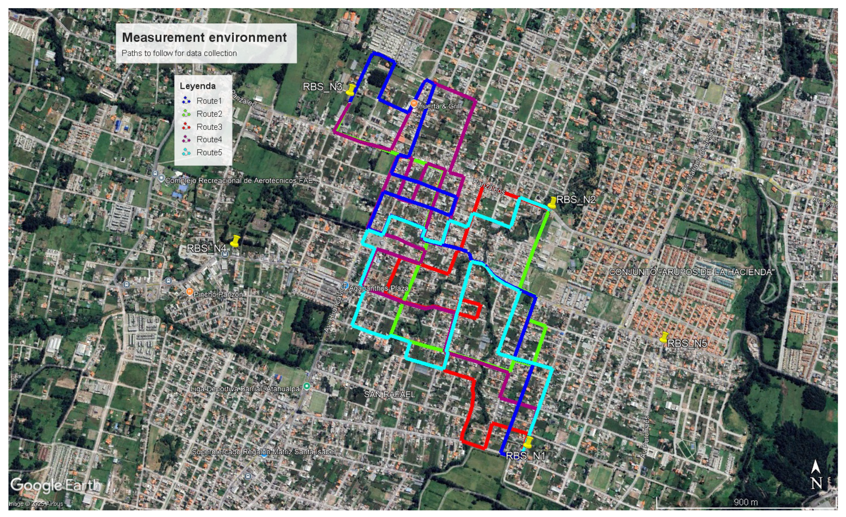
This section presents the results obtained after the full processing of the collected data, incorporating both statistical analysis and vector-based modeling in the urban and suburban study areas. To evaluate the behavior of radio-frequency parameters across different spatial conditions, a comprehensive statistical framework was applied. This included the calculation of the mean, standard deviation (SD), standard error (SE), and 95% confidence intervals (CIs) for each cell in the dataset, which allowed for the identification of signal quality patterns and the detection of anomalies in the coverage zones.

The analysis compared the power variation observed in the coverage area of a cellular network using two theoretical models—previously introduced in this study—and the experimental measurements collected in the field. Handover regions, specifically intra-handover and inter-handover events, were accurately detected using the methodology described in [4]. These identified zones were subsequently used to test the performance of the proposed vector-based theoretical approach to estimate the power variation as a function of the user terminal’s direction of movement.

Although the statistical evaluations and model validations were carried out in both urban and suburban environments, the initial focus of the discussion is on the urban scenario, as it presents more complex propagation conditions due to obstacles such as buildings and traffic density. Nonetheless, comparisons involving deviations between theoretical and experimental power estimates are provided for both environments in later sections, ensuring a comprehensive and balanced evaluation of the model’s performance.

The reference thresholds for classifying the quality levels of the main RF parameters analyzed in this work—RSSI, RSRQ, and RSSNR—are summarized in

Table 2. Thresholds considered in this study for the radio-frequency parameters.

Signal Quality	RSRP (dBm)	RSSI (dBm)	RSRQ (dB)	RSSNR (dB)
Excellent	≥$-80$	≥$-70$	≥$-10$	≥10
Good	$-90$ to $-80$	$-80$ to $-70$	$-10$ to $-15$	5 to 10
Fair	$-100$ to $-90$	$-95$ to $-80$	$-15$ to $-20$	0 to 5
Poor	≤$-100$	≤$-95$	≤$-20$	≤0

, serving as a benchmark for interpreting the results that follow.

4.1. Statistical Analysis of Radio-Frequency Parameter Measurements in the Coverage Area

Table 3. Statistics for RF parameters in urban and suburban environments within a coverage area.

Parameters	Urban				Suburban
	Mean	Min	Max	SD	Mean	Min	Max	SD
RSSI	−79.31	−120	−44	11.10	−97.00	−122	−54	12.00
RSRQ	−14.56	-20	−6	2.96	−14.70	−20	−3.6	3.10
RSSNR	1.20	−12	17	6.08	2.30	−12	14	5.30

,

Table 4. Statistics for RF parameters in urban and suburban environments within an intra-handover area.

Parameters	Urban				Suburban
	Mean	Min	Max	SD	Mean	Min	Max	SD
RSSI	−85.78	−119	−52	12.10	−90.60	−125	−70	11.90
RSRQ	−17.82	−20	−10	2.51	−14.60	−20	−7	2.50
RSSNR	−0.29	−12	7	6.36	2.27	−9	20	5.70

and

Table 5. Statistics for RF parameters in urban and suburban environments within an inter-handover area.

Parameters	Urban				Suburban
	Mean	Min	Max	SD	Mean	Min	Max	SD
RSSI	−89.89	−120	−56	10.01	−105.50	−123	−73	7.40
RSRQ	−18.39	−20	−11	2.09	−16.50	−20	−6	2.80
RSSNR	−0.40	−11	5	5.80	−2.40	−14	20	4.40

present the statistical analyses of the radio-frequency (RF) parameter measurements across the entire coverage area, as well as in the intra-handover and inter-handover zones, for both the urban and suburban scenarios considered.

In the urban area, the average values of RSSI and RSRQ fell within the good signal quality range, while the RSSNR reflected fair connection quality, according to the thresholds defined in Table 2. Conversely, in the suburban area, RSSI exhibited a poor average level, RSRQ remained within the good threshold, and RSSNR fell into the fair category—slightly better than in the urban setting, potentially due to lower interference and fewer physical obstructions.

In the intra-handover zones, the urban sector showed degradation in both signal strength and quality: RSSI and RSRQ dropped to fair levels, while RSSNR fell into the poor category, indicating increased instability during the handover process. In contrast, the suburban intra-handover zone exhibited more stable conditions, with RSSI and RSSNR averaging fair levels and RSRQ maintaining good quality. This suggests that although the suburban signal is generally weaker, it behaves more consistently during short-range mobility events.

For inter-handover zones—where transitions occur between more distant cells—the degradation was more pronounced. In the urban area, the average RSSI and RSRQ values were in the fair range, while RSSNR remained poor. In the suburban area, both RSSI and RSSNR fell into the poor category, and RSRQ dropped to the lower bound of the fair range. Notably, the standard deviation of RSSNR in the suburban area was slightly lower than in the urban area, suggesting less fluctuation, although the average quality remained poor.

Overall, the RSSI was stronger in the urban area, as expected due to the higher base station density and shorter average distances to transmitters. However, the suburban zone exhibited slightly better average RSSNR values in the general coverage area and intra-handover zones despite a weaker overall signal, suggesting reduced interference. The inter-handover zone in the suburban area was an exception, where the RSSNR degraded to below that in the urban zone, indicating localized interference or challenging propagation effects.

While our study focuses on the statistical behavior of signal strength and quality in intra- and inter-handover zones, it is worth noting that state-of-the-art methods—such as ray-tracing simulations, 3GPP-based stochastic models, and machine learning approaches—can provide precise power predictions under static conditions. However, these techniques often fail to capture dynamic power changes caused by terminal mobility, which our model explicitly accounts for through directional power estimation. Additionally, advanced technologies like stacked intelligent metasurfaces for direction-of-arrival (DoA) estimation [5,6] can help improve signal direction detection in dynamic scenarios.

Moreover, the data revealed that during handover events, the average received power typically decreased by about 7 dBm, with observed variations ranging from 5 to 10 dBm. This highlights the inherent instability in signal levels during cell transitions. Consequently, while the suburban area experienced a generally weaker and less stable signal strength, it occasionally benefited from lower interference, as reflected in certain improvements in the RSSNR and RSRQ, depending on the specific handover conditions and propagation characteristics.

4.2. Urban Area Results Using the Theoretical Channel Model

After presenting the theoretical analyses using two distinct approaches—one based on the decomposition and examination of Friis’s equation, as shown in Equation (7) (Theoretical Model 1), and the other employing vector calculus concepts, as detailed in Equation (24) (Theoretical Model 2)—it is pertinent to compare these models both with each other and with the experimental data obtained through NetMonitor measurements.

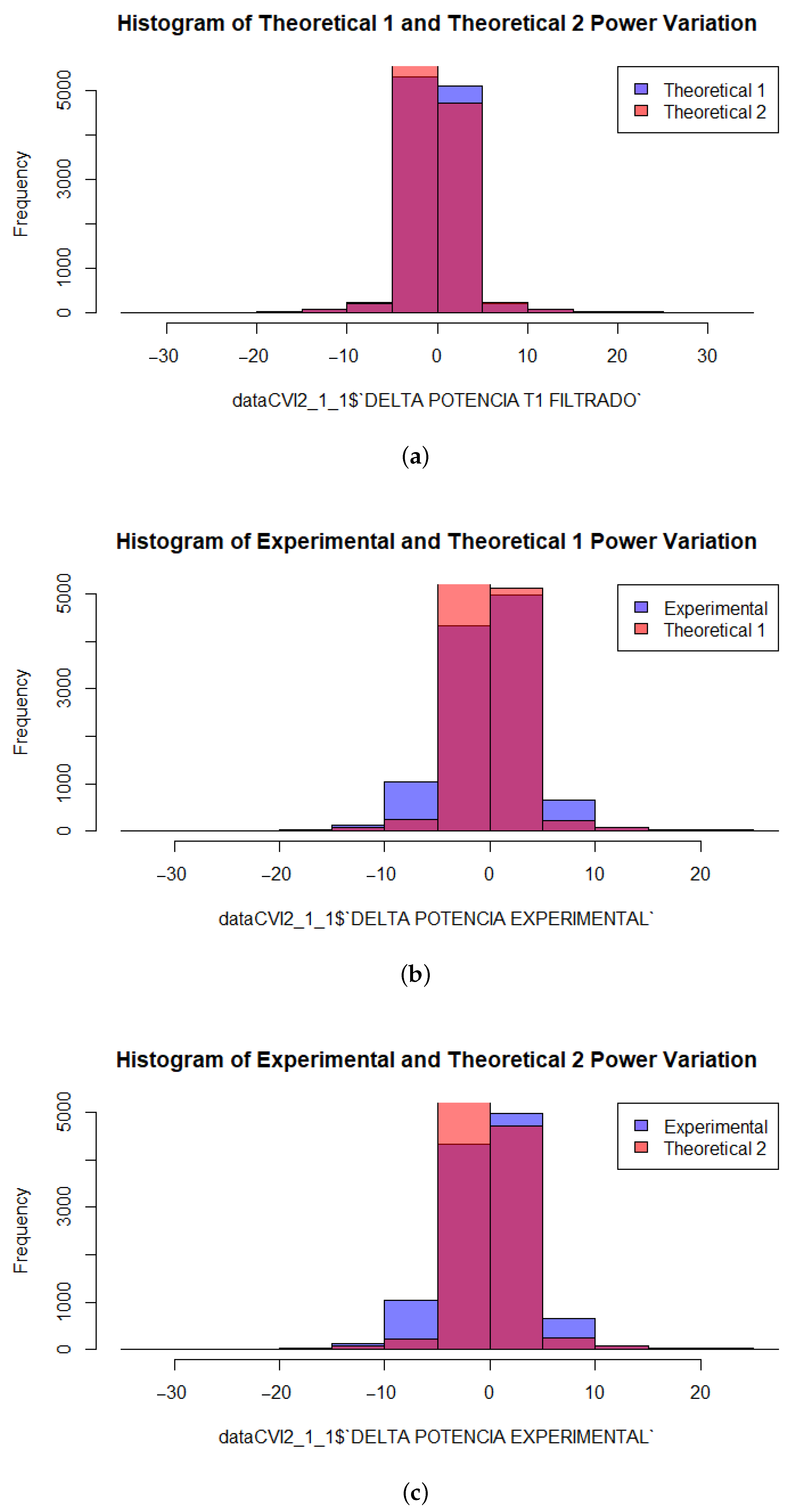
When comparing the results obtained from the two theoretical models, as shown in Figure 12a, the expected power variations are relatively small with respect to the movement of the user terminal. This behavior aligns with expectations, as both theoretical models consider only the position and movement direction of the user within the coverage area, without accounting for complex propagation phenomena such as fading, reflection, or diffraction.

In contrast, Figure 12b,c illustrate the theoretical and experimental power variations, respectively. The overlay of these distributions shows generally strong agreement: most samples yielded an error of less than 5%, indicating that the proposed model successfully captured the overall spatial trends of the signal variation. However, certain discrepancies can be observed, particularly in about 4% of the data, where abrupt power fluctuations occurred. These deviations are mostly concentrated around inter-handover regions, changes involving invalid or non-existent cells, or areas affected by measurement artifacts introduced by the NetMonitor software (version 1.81). This particular version, commonly used for LTE signal diagnostics, may produce placeholder values or incomplete readings under certain conditions, especially during cell transitions or low-coverage scenarios. This highlights the importance of robust data preprocessing in future implementations to improve accuracy.

The histograms in Figure 12 include a common color not defined in the legend table. This color represents overlapping measurement values common to both compared distributions, indicating zones where the theoretical and experimental results converge in power variation behavior.

Following this visual criterion, it can be observed that the comparison between the two theoretical models results in smaller power variation differences than when each theoretical model is compared individually against the experimental data. Nevertheless, even in the theoretical-to-experimental comparisons, the deviations remain relatively small, reinforcing the validity of the proposed approach.

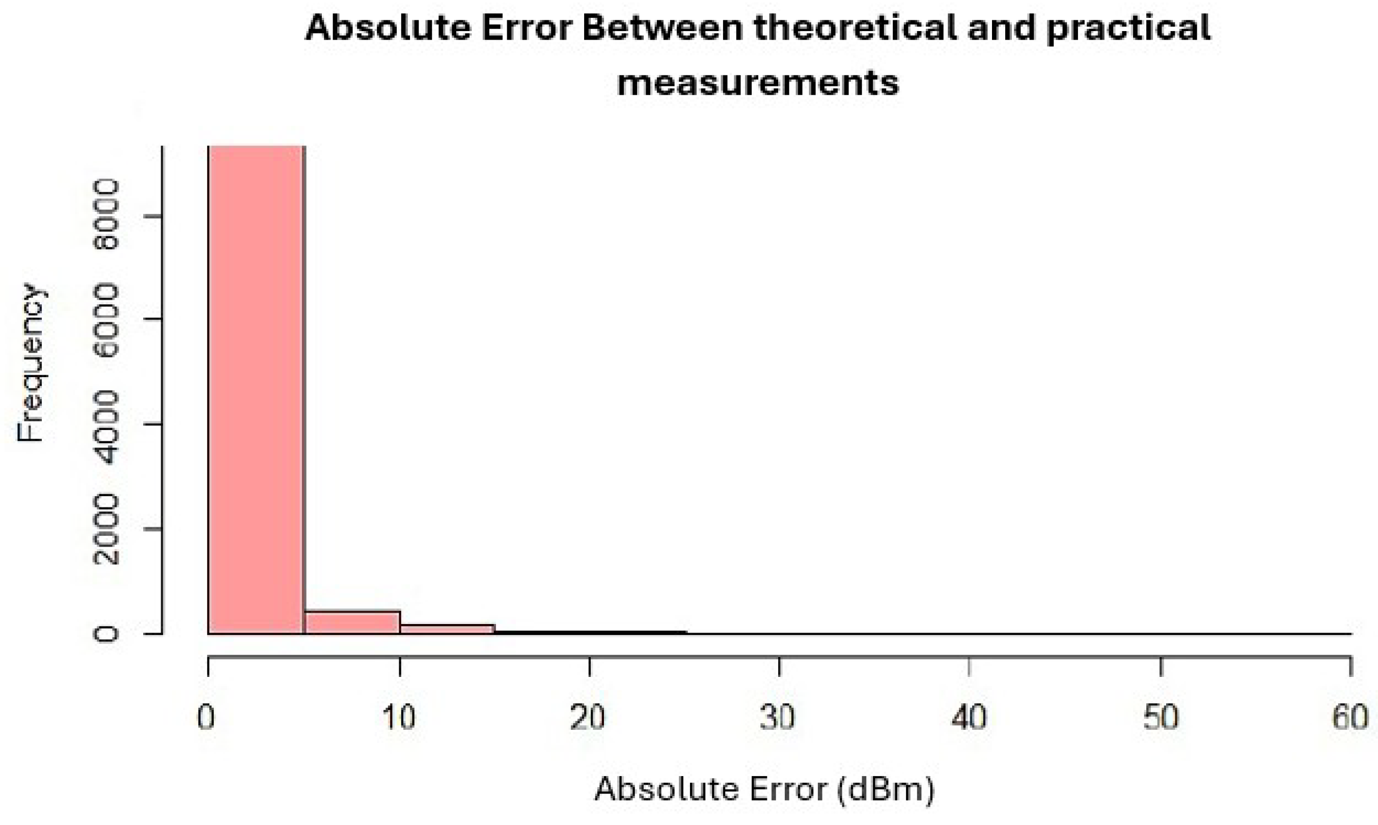
Furthermore, to assess the alignment between theoretical predictions and experimental results, a statistical analysis was conducted comparing the directional power variation derived from Equation (24) with the field measurements. As shown in Figure 13, the majority of measurement points—representing over 85% of the dataset—show a difference of less than 5 dBm between the theoretical and experimental values. This observation was statistically supported by an ANOVA test ($p<0.001$), which confirmed that the differences between the two groups (theoretical vs. experimental) were statistically significant but not substantial in magnitude. A post hoc Tukey test revealed that the average discrepancy between the matched theoretical and experimental values across the intra- and inter-handover zones ranged between 3.2 dBm and 3.5 dBm. Based on the maximum observed mean difference and relative to the overall dynamic range of the RSSI values in the dataset, the maximum cumulative error was conservatively estimated at 6.47% and did not exceed 7.6%.

From this point onward, the power variations obtained using Equation (24) are adopted, as they allow for the estimation of power trends based on the user terminal’s movement vector within the coverage area. This approach is consistent with the methodology previously described in the channel model section, where directional variations were incorporated to characterize propagation dynamics. Once the theoretical variation, $\Delta P_{\mathrm{Theo}}$, is determined, the predicted power at the next location, $P_{2_{\mathrm{Theo}}}$, can be estimated using the experimentally observed power at the previous point, $P_{1_{\mathrm{Exp}}}$, following Equation (26):

$$P_{2_{Theo}}\left[\mathrm{dBm}\right]=P_{1_{Exp}}\left[\mathrm{dBm}\right]+\Delta P_{Theo}\left[\mathrm{dBm}\right]$$

(26)

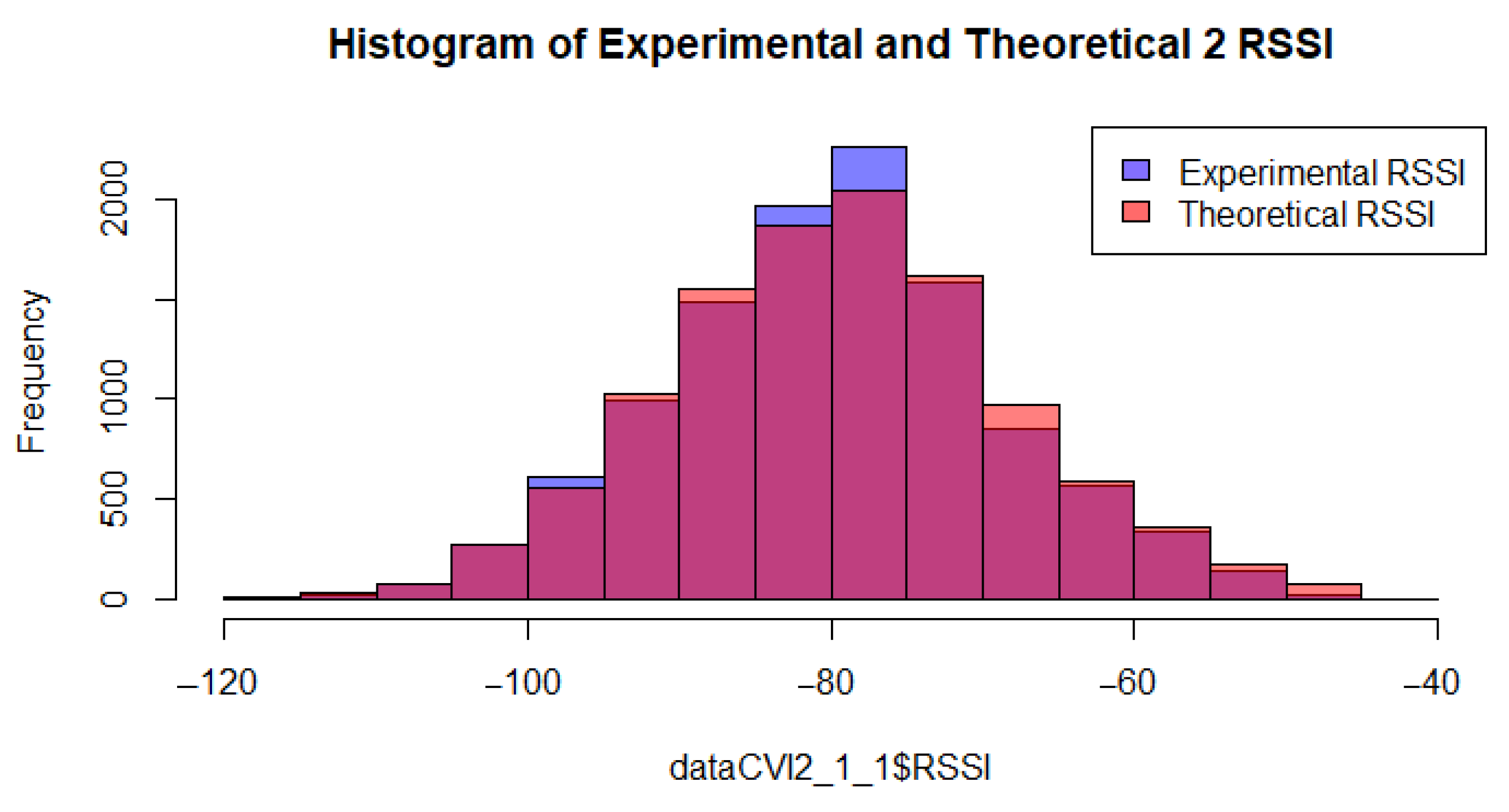
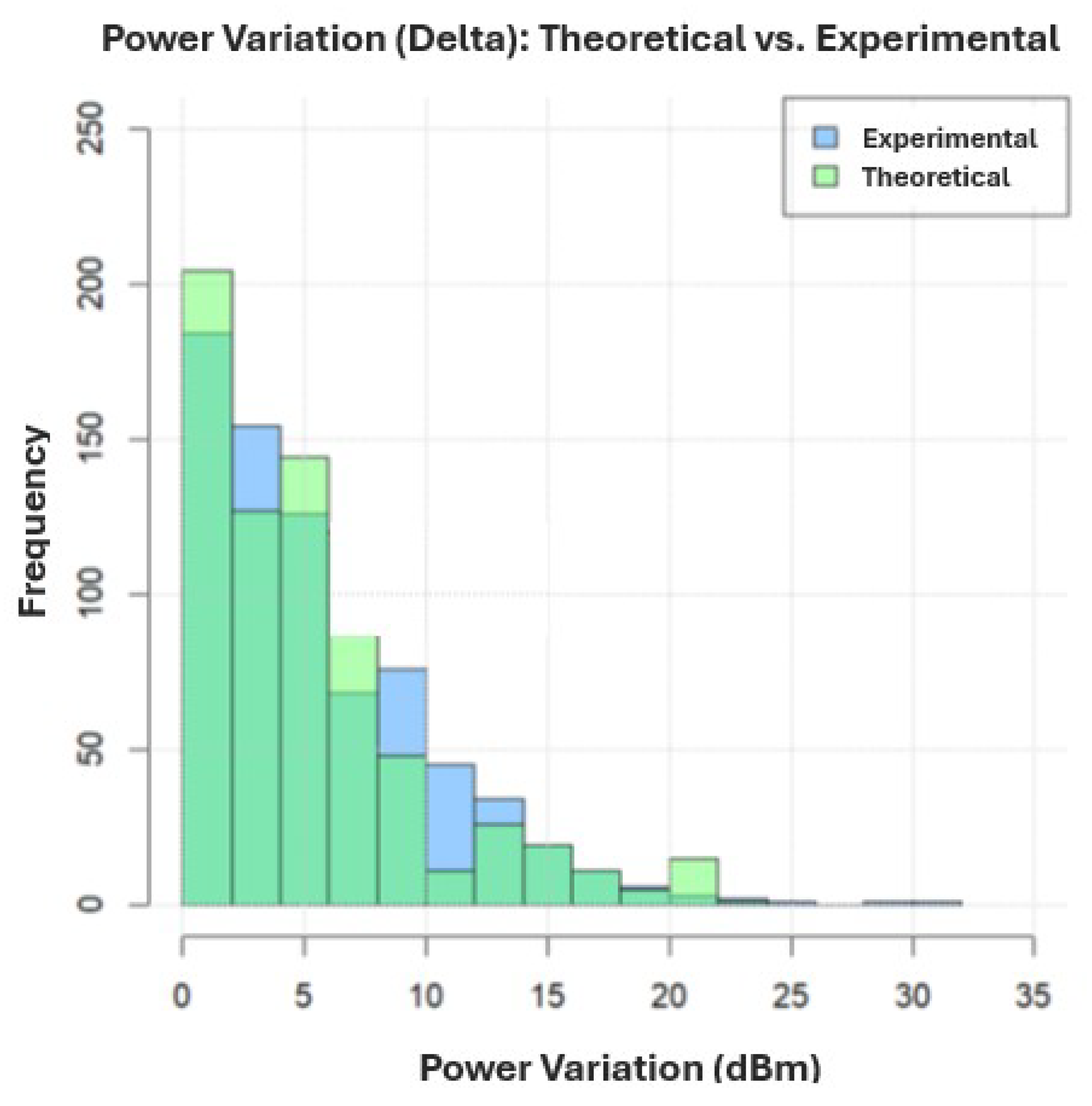
Following this approach, Figure 14 presents a comparative histogram illustrating the received signal strength indicator (RSSI) obtained experimentally using NetMonitor and the RSSI estimated by the proposed vector-based theoretical model. Both datasets exhibit a similar central tendency, particularly between $-80\mathrm{dBm}$ and $-75\mathrm{dBm}$, indicating that the model reliably approximates real-world signal behavior under average propagation conditions. This alignment is particularly evident in the urban scenario, where the base station density is higher and the propagation variability is somewhat reduced. However, the histogram also shows that the experimental RSSI values are more widely dispersed, especially toward lower power levels (e.g., below $-80\mathrm{dBm}$), reflecting the influence of random environmental factors—such as shadowing from buildings, fast fading, and inter-cell interference—that are not fully captured by the theoretical formulation.

This behavior is consistent with the statistical findings discussed previously. In the urban area, the experimental RSSI values showed an average of $-79.31\mathrm{dBm}$ with a standard deviation of $11.10\mathrm{dB}$, while in the suburban area, the mean RSSI dropped to $-97.00\mathrm{dBm}$, with greater dispersion ($12.00\mathrm{dB}$). Such degradation and variability were especially pronounced in the inter-handover zones of the suburban scenario, where both the RSSI and RSSNR were classified as poor, highlighting instability and increased susceptibility to interference. These statistical patterns help explain the histogram’s left-skewed tail, particularly in suburban transitions or areas with sparser infrastructure.

The comparison underscores both the strengths and limitations of the proposed model. On the one hand, it effectively replicated dominant propagation trends with a low average estimation error, not exceeding 7.6% under nominal conditions. On the other hand, it tended to underestimate the received power under non-ideal conditions—such as abrupt terrain variations, handovers, or interference from neighboring cells—especially in suburban areas, where long distances and fewer obstacles yielded higher path loss but also more variability in the RSSNR. Despite these deviations affecting only a minority of data points, the model remains a valuable tool for preliminary signal mapping and handover zone characterization, particularly in urban environments where rapid estimation is prioritized and full drive test datasets may be unavailable.

Unlike high-complexity models based on ray tracing or machine learning, which often require extensive parameter tuning, our low-complexity directional approach accurately captures real-time power fluctuations caused by terminal mobility. While advanced techniques such as those in [5,6] offer high angular resolution and spatial sensing for signal directionality, they do not explicitly model the temporal dynamics of the received power. Thus, our model complements such methods by focusing on directional transitions during motion, which are critical to mobile communication planning and handover optimization.

On the other hand, although the second theoretical model accurately predicted typical propagation patterns, it underrepresented extreme field conditions—particularly in suburban inter-handover zones—where sudden drops in the RSSI and increased standard deviations of the RSSNR suggest higher interference levels and less predictable power behavior.

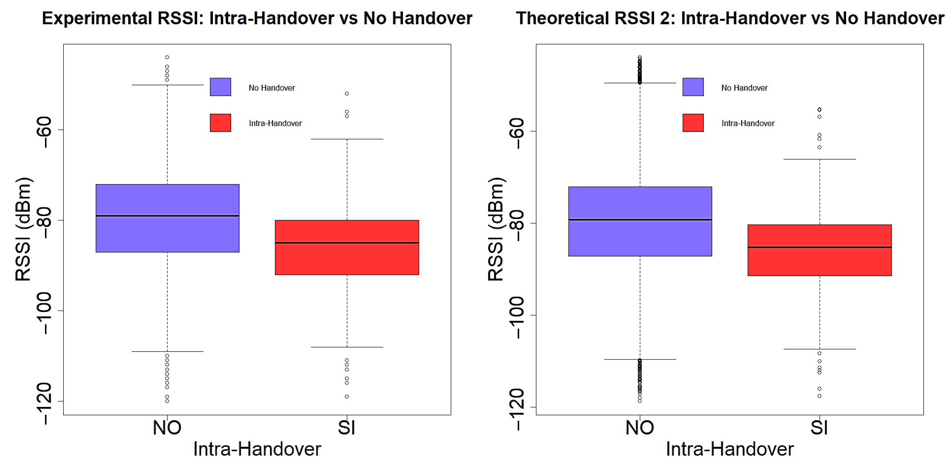
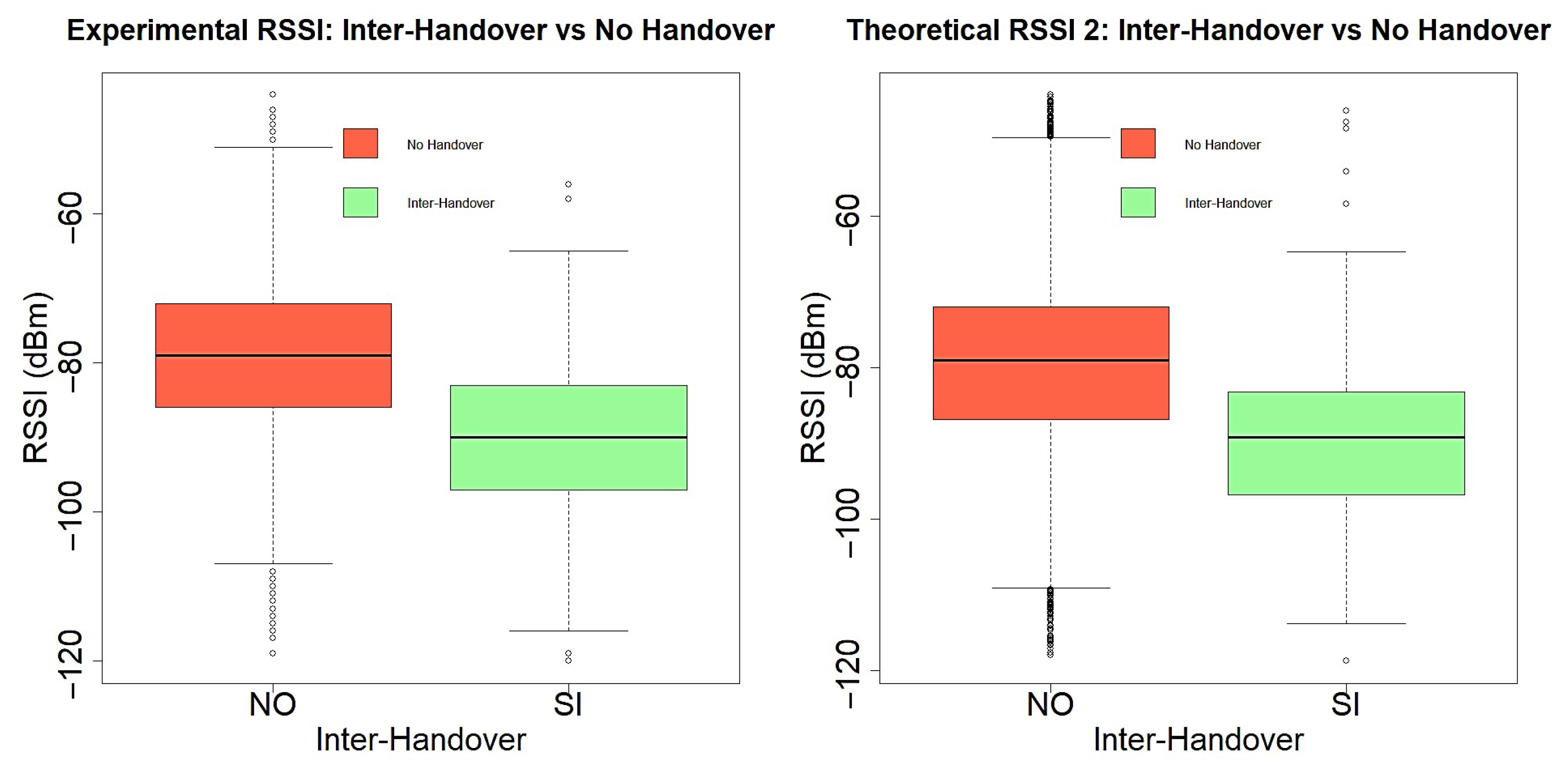
In this part of the analysis, the internal coverage areas of the cells are referred to as non-intra-handover and non-inter-handover cases. As expected, the graphs shown in Figure 15 and Figure 16 indicate that power levels are higher within the intra-handover zones than in the inter-handover zones.

As observed in both the experimental and theoretical cases, the mean values are very close, and the data distribution and dispersion exhibit similar patterns. This indicates that the applied method yielded results consistent with expectations.

By comparing the mean values of the experimental and theoretical RSSI in the urban environment, the results obtained are $-79.31\mathrm{dBm}$ and $-79.39\mathrm{dBm}$, respectively, with a relative error of less than 1%. This minimal discrepancy indicates a strong correlation between both sets of values and confirms the precision of the proposed vector-based model in estimating the received power under typical propagation conditions. Notably, the model achieved this level of accuracy without the need for site-specific calibration, training data, or computationally demanding simulations, distinguishing it from ray-tracing and machine learning-based models. While advanced DoA estimation techniques leveraging intelligent metasurfaces [5,6] offer superior angular resolution, they are not optimized for continuous power prediction in dynamic mobile scenarios. Nonetheless, these technologies could complement our approach by supplying accurate spatial orientation data, enabling hybrid models that incorporate both directionality and temporal power variation.

Furthermore, statistical validation through the analysis of variance (ANOVA) confirmed the significant impact of mobility events on signal strength. For the intra-handover process, the ANOVA test yielded a highly significant effect on RSSI values ($p=1.85\times {10}^{-11}$). The Tukey post hoc analysis revealed a mean RSSI difference of $-6.55\mathrm{dB}$ between the handover and non-handover conditions, with a 95% confidence interval of $[-8.45,-4.64]$, clearly excluding zero. Similarly, for the inter-handover scenario, the effect on the RSSI was even more pronounced ($p<2\times {10}^{-16}$), with a mean difference of $-10.94\mathrm{dB}$ and a 95% confidence interval of $[-12.08,-9.80]$. These results confirm that handover processes, especially inter-cell ones have a statistically significant and substantial impact on the received signal strength.

Additionally, Tukey’s post hoc comparisons between the theoretical and experimental RSSI values indicated statistically significant differences under specific mobility conditions. In the inter-handover zone under the SI–SI scenario (i.e., both theoretical and experimental handover detections were positive), the average difference was $3.21\mathrm{dB}$ ($p=0.0021$) with a confidence interval of $[1.17,5.25]$, indicating a moderate but statistically relevant discrepancy. In the NO–NO scenario (no handover detected in either case), the difference increased to $3.47\mathrm{dB}$ ($p<0.001$) with a tighter confidence interval of $[3.05,3.87]$, suggesting a consistent and systematic divergence between both models outside of mobility zones.

Overall, the integration of descriptive and inferential statistical methods supports the validity of the proposed model, particularly in urban environments.

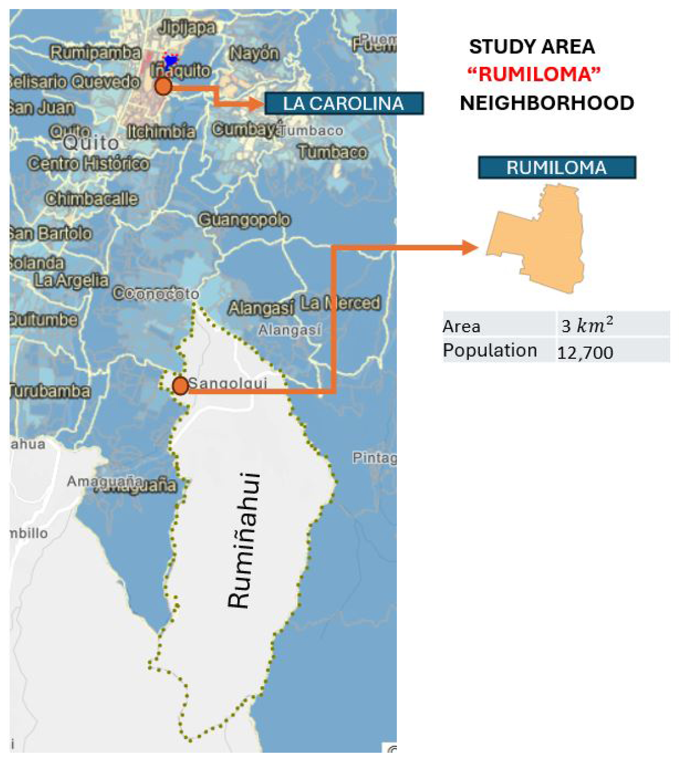
4.3. Suburban Area Results

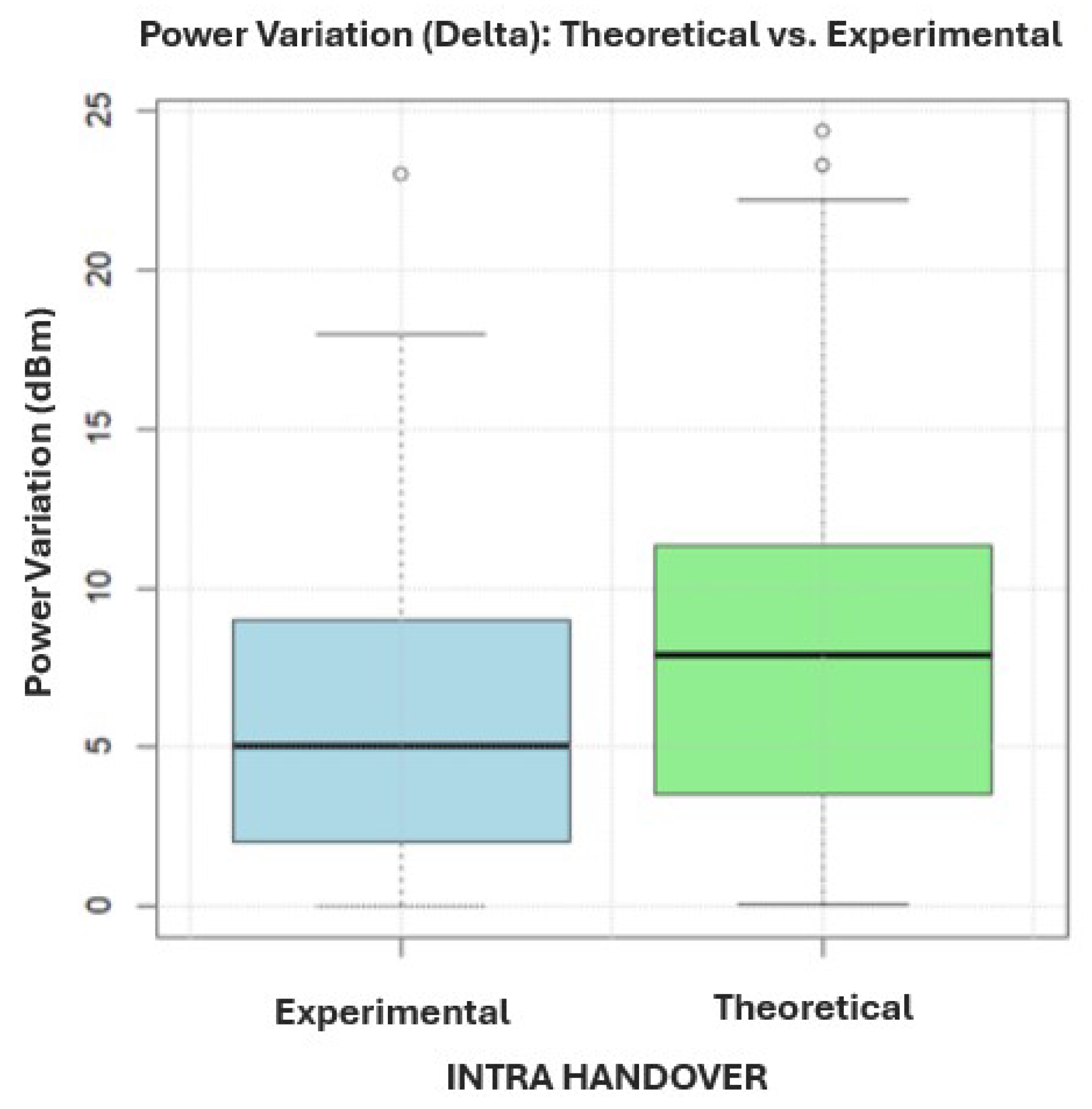
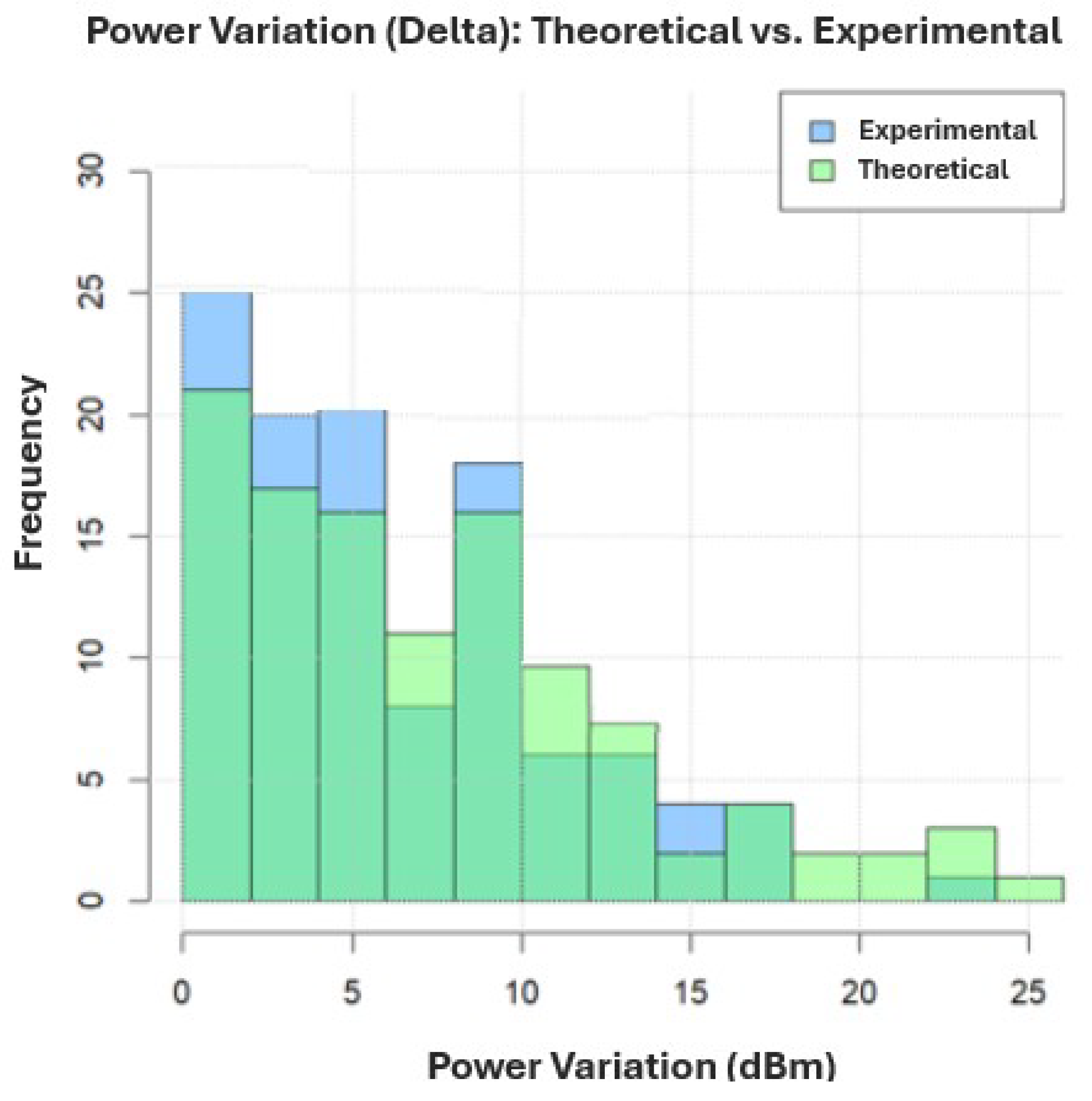
Figure 17 shows that in suburban intra-handover zones, the experimental power variation (difference between two consecutive measurement points) is predominantly concentrated between 0 and $5\mathrm{dBm}$, indicating that small power changes are the most frequent. The theoretical values also show peaks in this range and additionally in the $8.7$ to $11.2\mathrm{dBm}$ interval, although with fewer samples. Notably, some higher variation ranges (around 20 to $25\mathrm{dBm}$) appear only in the theoretical data, likely due to the absence of experimental samples in those intervals. This suggests that the theoretical results have a broader distribution, especially toward medium and large power variations, which are less common in practice.

Figure 18 complements this by illustrating that the experimental median variation is $5\mathrm{dBm}$, splitting the data evenly. The experimental distribution is positively skewed, with greater dispersion among higher values. Conversely, the theoretical median is higher at $7.8\mathrm{dBm}$ and shows a negative skew, with a greater spread in the lower half of the data and a concentration toward higher values. The theoretical box plot also presents more extreme values, as indicated by the longer upper whisker.

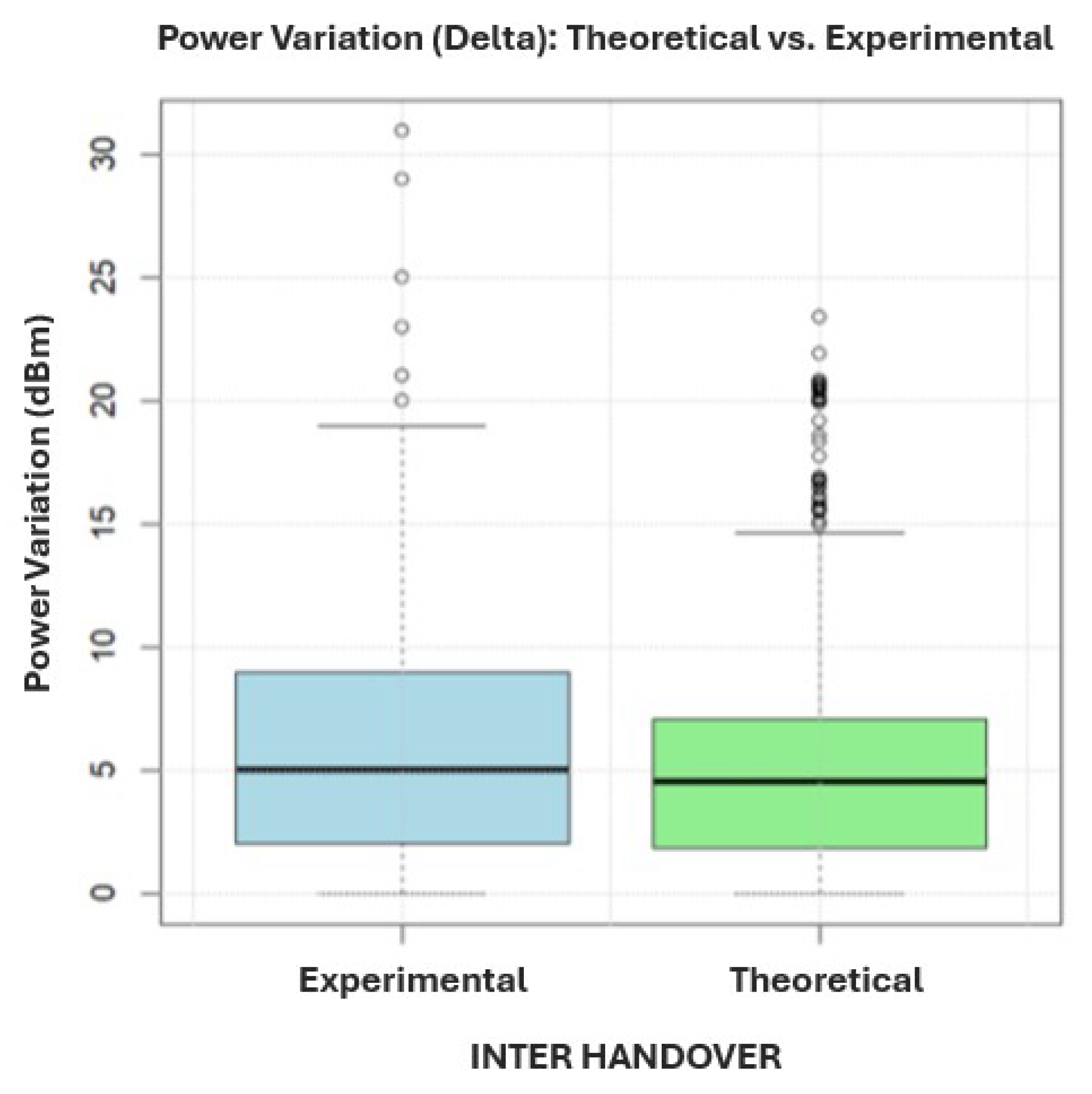
In the suburban inter-handover zones, Figure 19 shows that both the theoretical and experimental data are mainly concentrated between 0 and $6\mathrm{dBm}$, indicating that small changes predominate. However, while the theoretical data exhibit a peak around $6\mathrm{dBm}$, the experimental data are more evenly distributed across 6 to $11\mathrm{dBm}$. Additionally, the experimental data include outliers exceeding $30\mathrm{dBm}$, reflecting occasional abrupt power changes not fully captured by the model.

Figure 20 further shows the experimental median at $5\mathrm{dBm}$ with a positively skewed distribution and several outliers above $25\mathrm{dBm}$. The theoretical median is slightly lower at $4.5\mathrm{dBm}$ and shows a negative skew, with a greater dispersion in the lower range and outliers up to $15\mathrm{dBm}$, although less extreme than the experimental ones.

Overall, while the theoretical model captures the general behavior of power variations in suburban environments, it exhibits somewhat larger deviations than in urban settings, particularly with respect to higher-magnitude fluctuations during handovers. This reflects the more complex and variable propagation conditions typical of suburban areas.

4.4. Evaluation of the Performance of the Theoretical Model

This section evaluates the accuracy of the proposed theoretical model in estimating the received signal power at the user terminal’s next position, based on its movement vector and previously measured power. The analysis compared the theoretical predictions with the experimental measurements across three types of coverage areas: fully covered zones, intra-handover zones, and inter-handover transition zones.

Table 6. Relative error in the theoretical estimation of the received power $P_2$ within fully covered areas.

Power Estimation P2	Urban	Suburban
Relative Error	4.8%	5.3%

,

Table 7. Relative error in the theoretical estimation of the received power $P_2$ within intra-handover zones.

Power Estimation P2	Urban	Suburban
Relative Error	5.2%	5.6%

and

Table 8. Relative error in the theoretical estimation of the received power $P_2$ within inter-handover zones.

Power Estimation P2	Urban	Suburban
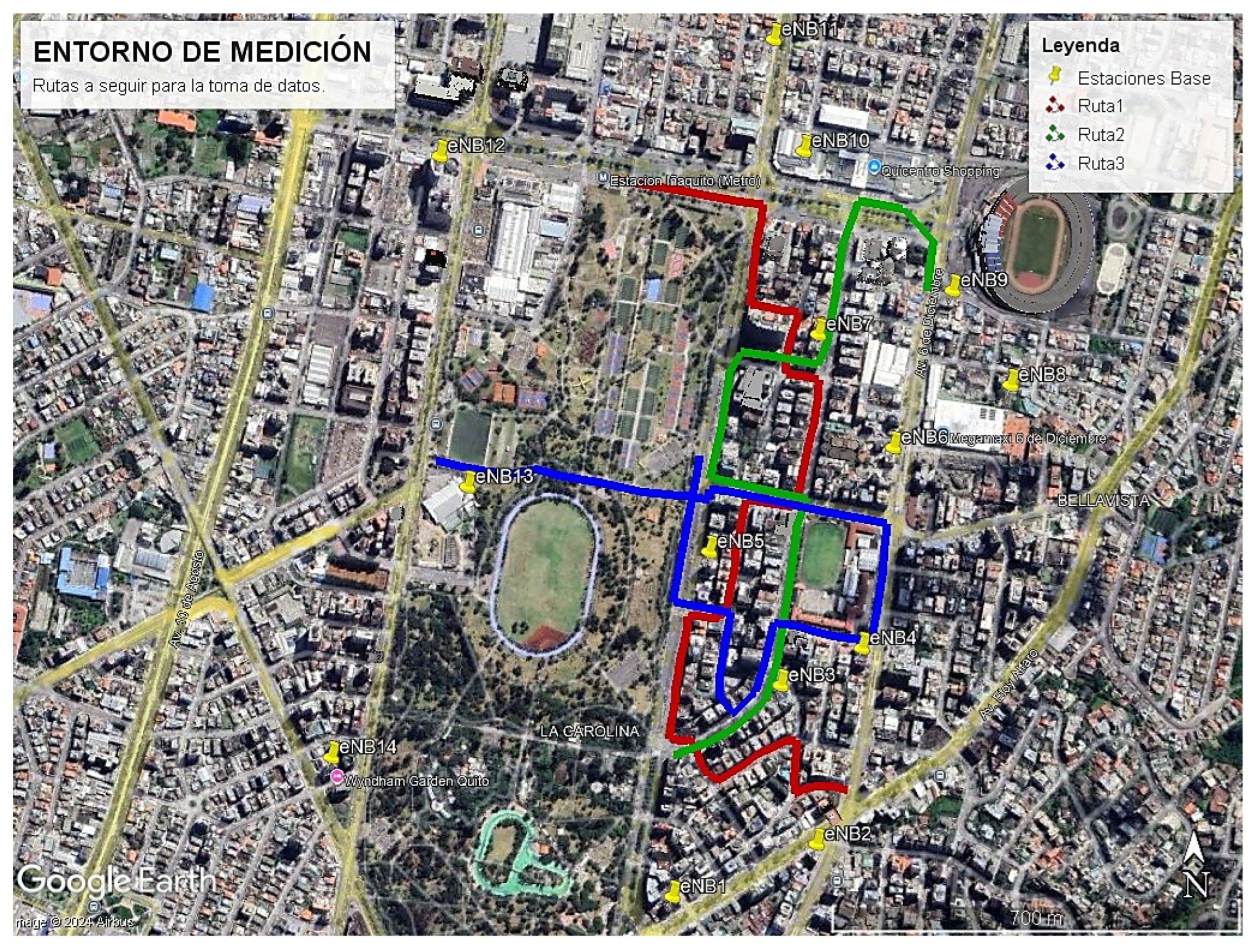
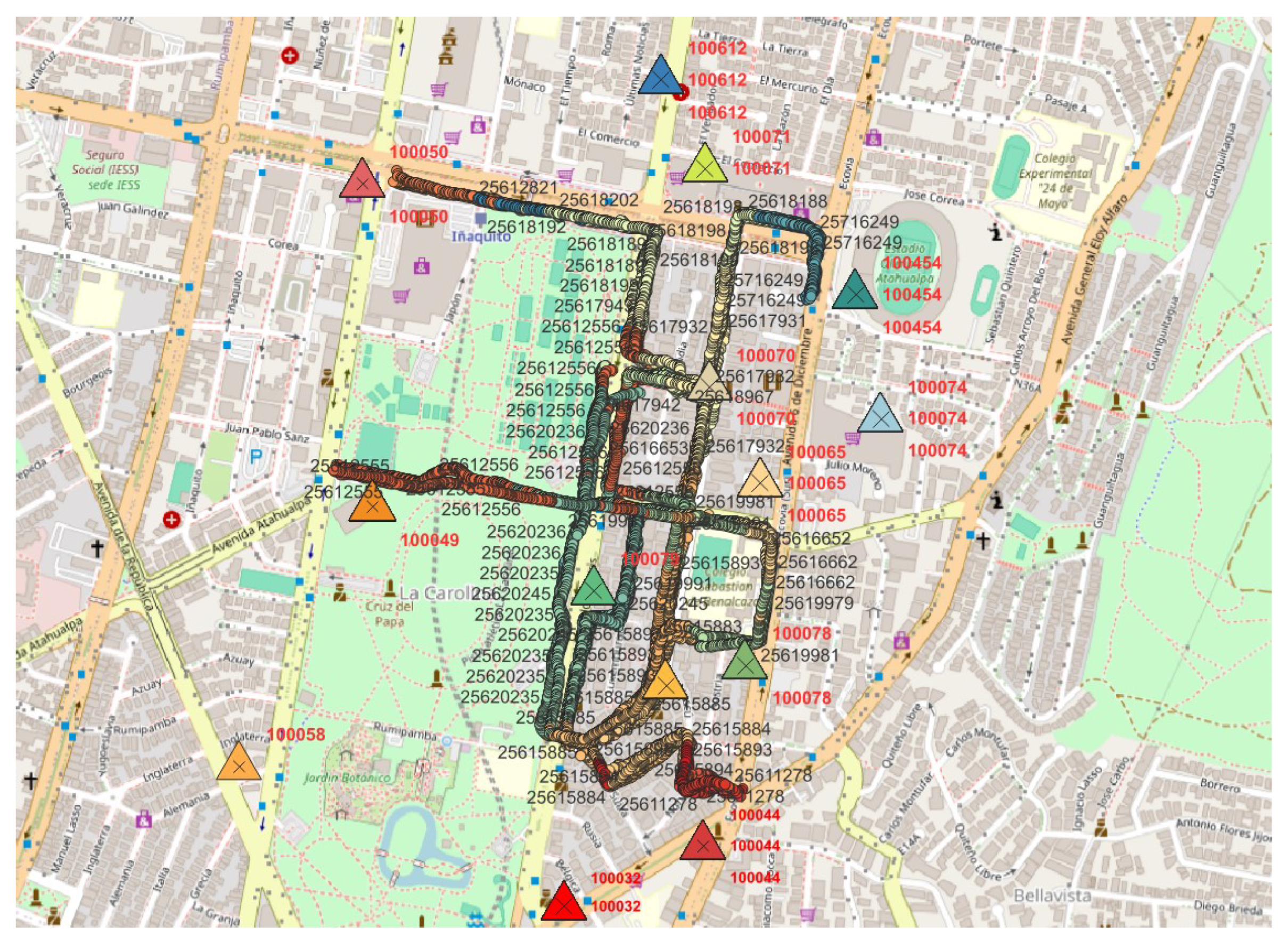
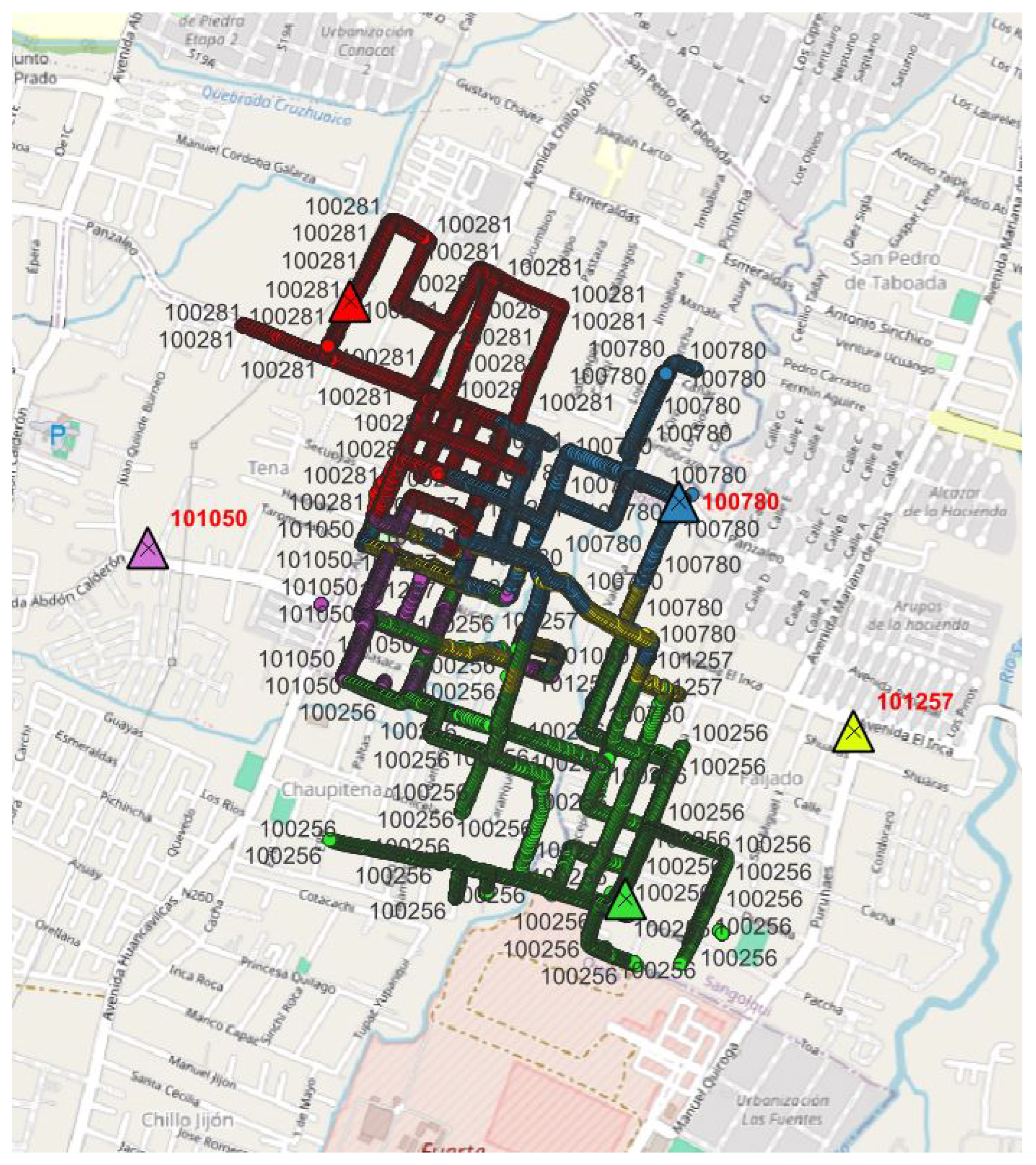
Relative Error	6.3%	7.6%

summarize the relative error between the theoretical and experimental power values for each case. These values were computed over 11,253 georeferenced measurements from 14 urban base stations covering 59 sectors. Data inconsistencies (e.g., missing or corrupted values) in the dataset were excluded from the final analysis, the criteria for which were discussed in the data processing section.

To statistically evaluate the agreement between the theoretical predictions and the measured values, an ANOVA test was conducted across all zones and scenarios. The test revealed statistically significant differences between the theoretical and experimental groups ($p<0.001$), although the effect size was relatively small. A post hoc Tukey HSD test indicated that the average discrepancy across all measurements remained between 3.2 dBm and 3.5 dBm. Over 85% of the data points showed a deviation of less than 5 dBm, which was adopted as a practical threshold for acceptable model accuracy.

Based on this threshold and considering the overall dynamic range of the RSSI values in the dataset, the maximum cumulative relative error was conservatively estimated at 6.47%. This value reflects a statistically bounded upper limit for error under typical operational conditions, validating the model’s utility for real-world applications.

It is also evident that errors increased progressively from fully covered zones to intra-handover and inter-handover zones. This trend correlates with the presence of complex propagation effects, such as interference and fast fading, which are more prominent during cell transitions. Notably, suburban areas consistently showed slightly higher errors than urban zones. This can be attributed to the broader coverage footprints and reduced antenna density in suburban deployments, which introduced additional variability not captured by the model’s current assumptions (e.g., flat terrain, horizontal radiation pattern, and constant gain).

In summary, the proposed model demonstrates consistent and robust predictive capabilities. Its relative error remains within acceptable bounds across diverse environments, making it a suitable analytical tool for rapid power estimation, especially in scenarios where detailed infrastructure data are unavailable.

4.5. Model Applicability and Complexity

The proposed model distinguishes itself through its simplicity and practical applicability in real-world scenarios. It is founded on well-established theoretical principles, including Friis’ transmission equation and large-scale path-loss models, requiring only a limited set of empirical signal measurements collected via commonly available tools. Unlike more complex methods that depend on detailed infrastructure data, 3D ray-tracing simulations, or advanced wave-domain processing techniques, this model facilitates mobility-aware signal estimation without incurring high computational costs or needing prior knowledge of environmental obstacles.

This reduced complexity renders the model particularly suitable for environments lacking comprehensive information about base station locations, building geometries, or full network topology. As demonstrated in the previous sections, the model attains estimation errors below 8% while maintaining low computational overhead. Moreover, by enabling the identification of handover zones and analyzing signal power variations associated with user movement, the model offers insights for optimizing network coverage.

5. Conclusions

The vector calculus-based analysis enabled the derivation of an estimation equation capable of predicting power levels at a given geographic coordinate with an accuracy of approximately 95%. This prediction, which relies on key parameters such as the mobile terminal’s movement direction and network characteristics, significantly reduces the need for extensive field measurements in these environments.

By applying vector calculus, it was possible to estimate the received power at a specific location based on the mobile terminal’s movement direction, defined by the angle $\theta$ and the traveled distance. This approach proved effective for analysis within the horizontal plane. The present study introduces a theoretical model grounded in vector calculus to estimate the received power at a point, given the known power at the preceding location and the direction of the mobile terminal’s movement. Estimating the received power at subsequent locations based on terminal movement is valuable, as it enables the determination of the terminal’s position within the coverage area and supports applications such as signal arrival direction assessment, identification of handover zones, and detection of reception issues. These capabilities can be leveraged to optimize network coverage through adaptive handover strategies and targeted enhancement interventions.

The model’s performance was evaluated in both urban and suburban environments, with estimation errors observed to be below 7.6%. Given the potential for improvement, future work will consider additional factors, including antenna radiation characteristics such as horizontal and vertical gains, as well as propagation conditions specific to the studied environments. For a more comprehensive analysis that incorporates vertical dimensions, future studies should also include parameters like the electrical and mechanical tilt of antennas.

Furthermore, the integration of automation techniques and machine learning algorithms presents opportunities to enhance model accuracy and adaptability. By training models on extensive empirical datasets and incorporating real-time measurement feedback, it will be possible to develop more precise and dynamic power estimation frameworks.

References

1. Wang, C.-X.; Bai, L.; Sun, S.; Ai, B.; Zhang, Y.; Shafi, M. A Survey of 5G Channel Measurements and Models. IEEE Commun. Surv. Tutor. 2021, 24, 3142–3168. [Google Scholar] [CrossRef]
2. El-Saleh, A.A.; Alhammadi, A.; Shayea, I.; Hassan, W.H.; Honnurvali, M.S.; Daradkeh, Y.I. Measurement Analysis and Performance Evaluation of Mobile Broadband Cellular Networks in a Populated City. Alex. Eng. J. 2022, 66, 927–946. [Google Scholar] [CrossRef]
3. Raida, V.; Svoboda, P.; Rupp, M. Real World Performance of LTE Downlink in a Static Dense Urban Scenario—An Open Dataset. In Proceedings of the GLOBECOM 2020—2020 IEEE Global Communications Conference, Taipei, Taiwan, 7–11 December 2020; pp. 1–6. [Google Scholar] [CrossRef]
4. Espinosa, R.; Lupera-Morillo, P.; Farre, V.; Maldonado, R.; Llugsi Cañar, R. Statistical Analysis of Handover Process Performance in a Cellular Mobile Network in the City of Quito, Ecuador. Eng. Proc. 2023, 47, 19. [Google Scholar] [CrossRef]
5. An, J.; Yuen, C.; Di Renzo, M.; Debbah, M.; Poor, H.V.; Hanzo, L. Stacked Intelligent Metasurface Performs a 2D DFT in the Wave Domain for DOA Estimation. arXiv 2023, arXiv:2310.12345. Available online: https://www.researchgate.net/publication/374845149_Stacked_Intelligent_Metasurface_Performs_a_2D_DFT_in_the_Wave_Domain_for_DOA_Estimation (accessed on 23 June 2025).
6. Zhou, Y.; Zhang, J.; Yuen, C.; Wang, Y. Two-dimensional Direction-of-Arrival Estimation Using Stacked Intelligent Metasurfaces. IEEE Trans. Signal Process. 2023, 71, 4567–4580. Available online: https://www.researchgate.net/publication/381455226_Two-Dimensional_Direction-of-Arrival_Estimation_Using_Stacked_Intelligent_Metasurfaces (accessed on 23 June 2025).
7. 3GPP TR 38.901 V17.0.0 (2022-03): Study on Channel Model for Frequencies from 0.5 to 100 GHz (Release 17). 3rd Generation Partnership Project. Available online: https://www.3gpp.org/ftp/Specs/archive/38_series/38.901/ (accessed on 23 June 2025).
8. MacCartney, G.R.; Rappaport, T.S. Rural Macrocell Path Loss Models for Millimeter Wave Wireless Communications. IEEE J. Sel. Areas Commun. 2017, 35, 1663–1677. Available online: https://ieeexplore.ieee.org/document/7914696 (accessed on 24 June 2025). [CrossRef]
9. Wu, T.; Wang, C.-X.; Li, J.; Huang, C. Machine Learning-Based Predictive Channel Modeling for 6G Wireless Communications Using Image Semantic Segmentation. In Proceedings of the 2023 IEEE 34th Annual International Symposium on Personal, Indoor and Mobile Radio Communications (PIMRC), Toronto, ON, Canada, 5–8 September 2023; pp. 1–6. [Google Scholar] [CrossRef]
10. Balanis, C.A. Antenna Theory: Analysis and Design, 3rd ed.; Wiley-Interscience: Toronto, ON, Canada, 2024. [Google Scholar]
11. Lupera-Morillo, P.; Parra, E.R. A Ray-Tracing Simulator for Predicting UHF Signals Propagation in Tunnels (Case Study Metro of Quito). In Proceedings of the 2020 IEEE ANDESCON, Quito, Ecuador, 13–16 October 2020; pp. 1–6. [Google Scholar] [CrossRef]
12. Larson, R.; Edward, B.H. Cálculo 2 de Varias Variables, 9th ed.; McGraw-Hill Interamericana Editores: Mexico City, Mexico, 2010. [Google Scholar]
13. Tello-Cedeño, K.; Carrera, J.; Meneses, M.; García, F. Estimación del ángulo de orientación de celdas celulares en redes LTE a partir de datos de medición. Rev. Publicando 2023, 10, 412–430. [Google Scholar]
14. Montgomery, D.C. Design and Analysis of Experiments, 9th ed.; Wiley: Hoboken, NJ, USA, 2017. [Google Scholar]
15. Polak, L.; Kufa, J.; Sotner, R.; Fryza, T. Measurement and Analysis of 4G/5G Mobile Signal Coverage in a Heavy Industry Environment. Sensors 2024, 24, 2538. [Google Scholar] [CrossRef] [PubMed]
16. Shayea, I.; Benlakehal, M.E.; Azmi, M.H.; Han, C.T.; Arsad, A.; Rahman, T.A. Outdoor Mobile Broadband Performance Analysis in Malaysia, Singapore, and Thailand. Results Eng. 2024, 23, 102691. [Google Scholar] [CrossRef]
17. Crawley, M.J. The R Book, 2nd ed.; Wiley: Hoboken, NJ, USA, 2012. [Google Scholar]
Figure 1. Graph of the theoretical power derivative with respect to the theta variable vs. the HPBW.
Electronics 14 03077 g001
Figure 2. Graph of the theoretical power derivative with respect to distance vs. distance.
Electronics 14 03077 g002
Figure 3. General methodology for data collection and analysis.
Electronics 14 03077 g003
Figure 4. Flowchart of the measurement methodology.
Electronics 14 03077 g004
Figure 5. “La Carolina” neighborhood, Iñaquito parish.
Electronics 14 03077 g005
Figure 6. Selected routes for data collection and base stations in the urban area.
Electronics 14 03077 g006
Figure 7. Selected routes for data collection and base stations in the urban area. Each color corresponds to the serving base station associated with the measured data along that route segment.
Electronics 14 03077 g007
Figure 8. “Rumiloma” neighborhood, suburban area.
Electronics 14 03077 g008
Figure 9. Selected routes for data collection and base stations in the suburban area.
Electronics 14 03077 g009
Figure 10. Selected routes for data collection and base stations in the suburban area. Each color corresponds to the serving base station associated with the measured data along that route segment.
Electronics 14 03077 g010
Figure 11. Model of a three-sector base station.
Electronics 14 03077 g011
Figure 12. Comparison of the histograms obtained in the study. (a) Histogram of power delta—Theoretical Model 1 vs. Theoretical Model 2. (b) Histogram of power delta—experimental vs. Theoretical Model 1. (c) Histogram of power delta—experimental vs. Theoretical Model 2.
Electronics 14 03077 g012
Figure 13. Histogram of the absolute error between the theoretical and experimental power variations. Approximately 2000 data points show significant deviations.
Electronics 14 03077 g013
Figure 14. Comparative histogram of experimental and theoretical power 2, estimated based on the direction of movement for consecutive points.
Electronics 14 03077 g014
Figure 15. Comparison of experimental RSSI and theoretical RSSI in intra-handover and non-intra-handover cases.
Electronics 14 03077 g015
Figure 16. Comparison of experimental RSSI and theoretical RSSI in inter-handover and non-inter-handover cases.
Electronics 14 03077 g016
Figure 17. Histogram of theoretical and experimental power variations in suburban intra-handover zones.
Electronics 14 03077 g017
Figure 18. Box plot of theoretical and experimental power variations in suburban intra-handover zones.
Electronics 14 03077 g018
Figure 19. Histogram of theoretical and experimental power variations in suburban inter-handover zones.
Electronics 14 03077 g019
Figure 20. Box plot of theoretical and experimental power variations in suburban inter-handover zones.
Electronics 14 03077 g020