Short-Term Prediction Intervals for Photovoltaic Power via Multi-Level Analysis and Dual Dynamic Integration

Abstract

There is an obvious correlation between the photovoltaic (PV) output of different physical levels; that is, the overall power change trend of large-scale regional (high-level) stations can provide a reference for the prediction of the output of sub-regional (low-level) stations. The current PV prediction methods have not deeply explored the multi-level PV power generation elements and have not considered the correlation between different levels, resulting in the inability to obtain potential information on PV power generation. Moreover, traditional probabilistic prediction models lack adaptability, which can lead to a decrease in prediction performance under different PV prediction scenarios. Therefore, a probabilistic prediction method for short-term PV power based on multi-level adaptive dynamic integration is proposed in this paper. Firstly, an analysis is conducted on the multi-level PV power stations together with the influence of the trend of high-level PV power generation on the forecast of low-level power generation. Then, the PV data are decomposed into multiple layers using the complete ensemble empirical mode decomposition with adaptive noise (CEEMDAN) and analyzed by combining fuzzy entropy (FE) and mutual information (MI). After that, a new multi-level model prediction method, namely, the improved dual dynamic adaptive stacked generalization (I-Stacking) ensemble learning model, is proposed to construct short-term PV power generation prediction models. Finally, an improved dynamic adaptive kernel density estimation (KDE) method for prediction errors is proposed, which optimizes the performance of the prediction intervals (PIs) through variable bandwidth. Through comparative experiments and analysis using traditional methods, the effectiveness of the proposed method is verified.

1. Introduction

Energy is not only the foundation of economic development, but also plays an important role in addressing climate change and energy transition [1,2]. With the gradual depletion of fossil fuels and the growing call for environmental protection, the utilization of clean and renewable energy has become a global consensus [3]. Among these energy sources, solar PV power generation is regarded as one of the key technologies in the future energy field. The application of PV energy is becoming increasingly widespread, and accurately predicting PV power generation has become particularly important [4,5]. However, PV power generation is susceptible to natural factors such as weather, season, and climate, and is characterized by volatility and uncertainty [6,7]. How to predict PV output efficiently has become a key issue in power grid dispatching. Therefore, accurate and reliable PV output prediction is of great value for the implementation of power grid dispatching and ensuring the stable and safe operation of PV power stations [8].

In recent years, with the advancement of prediction technology, the scale of PV power generation projects has been continuously expanding, demonstrating a promising development prospect [9]. At present, there have been relatively mature studies on PV power prediction methods, such as statistical methods [10], which have simple principles and are easy to implement. However, when the sample data are relatively complex, the prediction effect is average. Another type of method is machine learning algorithms [11], such as random forest (RF) [12], extreme learning machine (ELM) [13], and support vector machine (SVM) [14]. However, single-layer neural network prediction models are difficult to meet the prediction requirements. Deep learning methods can effectively solve these problems. Deep learning networks such as long short-term memory (LSTM) [15] and convolutional neural networks (CNNs) [16] have gradually been applied in PV prediction. The features extracted by CNNs are used as the input of a recurrent neural network to achieve the prediction of PV power generation [17]. More accurate PV power prediction is achieved by using LSTM autoencoders [18]. However, a single model has difficulty handling complex data distributions and is prone to overfitting or underfitting during training.

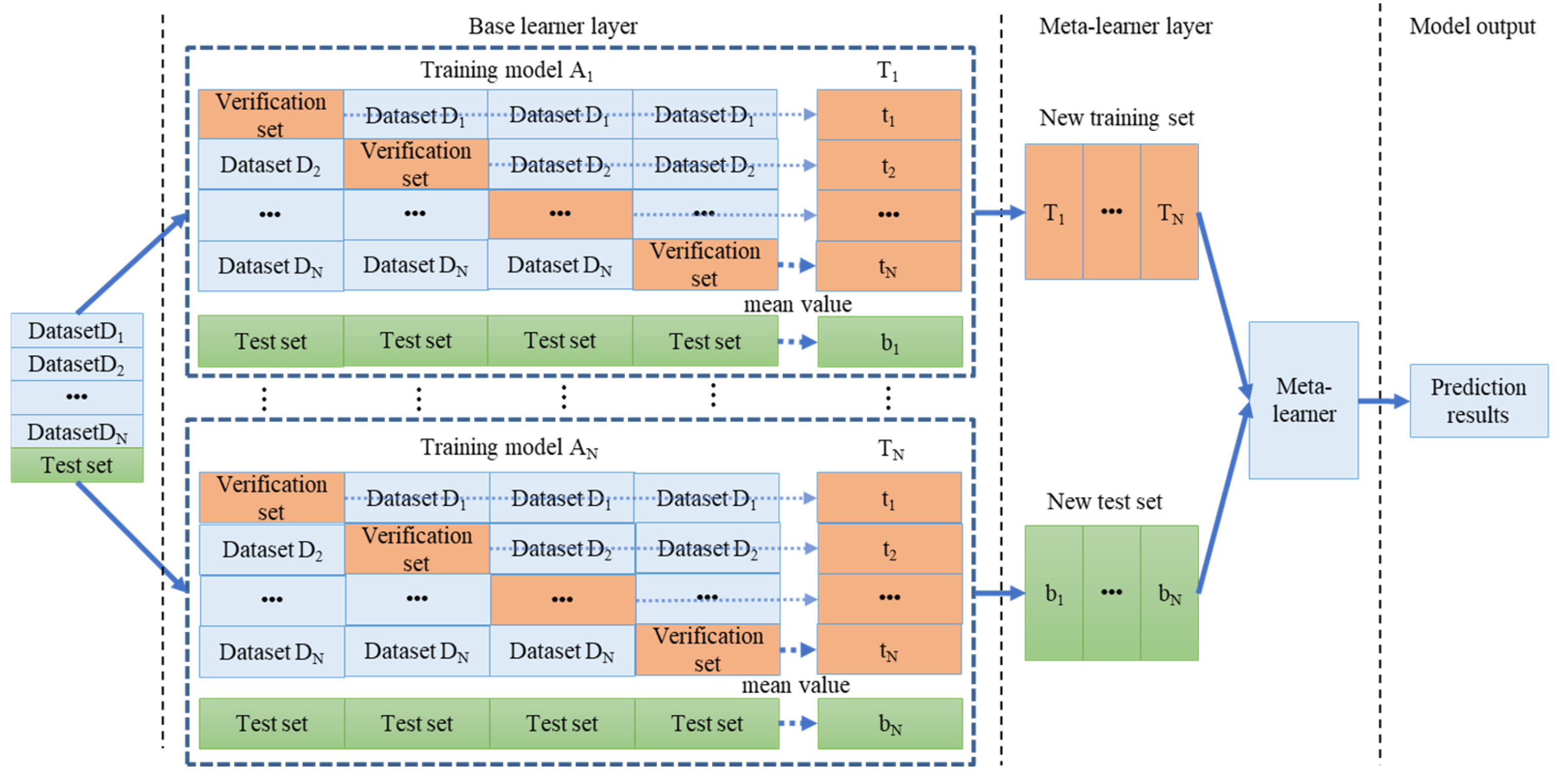
Ensemble learning captures more patterns and rules by integrating the prediction results of multiple base learners and has a stronger generalization ability. The PV production forecast is generated by using the basic models of four different LSTM architectures [19]. Two deep learning algorithms are utilized as the base learner, and the extreme gradient augmentation algorithm is used as the meta-learner to improve the accuracy of solar PV power generation prediction [20]. The three machine learning algorithms are integrated using the baseline linear regression model to achieve PV prediction. The results show that the integrated model is superior to the individual model [21]. A comparative analysis of the main features of various PV prediction technologies is shown in

Table 1. Analysis of PV prediction technology.

Method	Model	Features	References
Statistics	Regression analysis, time series analysis	The principle of this method is simple, but it cannot handle complex data.	[10]
Machine learning	RF, SVM, ELM, CNN, LSTM	This method can handle complex data but is prone to overfitting or underfitting.	[11,12,13,14,15,16,17,18]
Ensemble learning	Stacking, XGBoost	This method has strong robustness and high generalization ability, but lacks adaptability.	[19,20,21]

. However, the traditional stacking method adopts a fixed learner and lacks dynamic adjustment, which limits the model performance and prediction accuracy when dealing with complex and variable PV prediction scenarios. Therefore, it is necessary to explore a dynamic adaptive ensemble learning framework to improve the model’s adaptability and generalization ability, which is of great significance for enhancing the performance of PV prediction models.

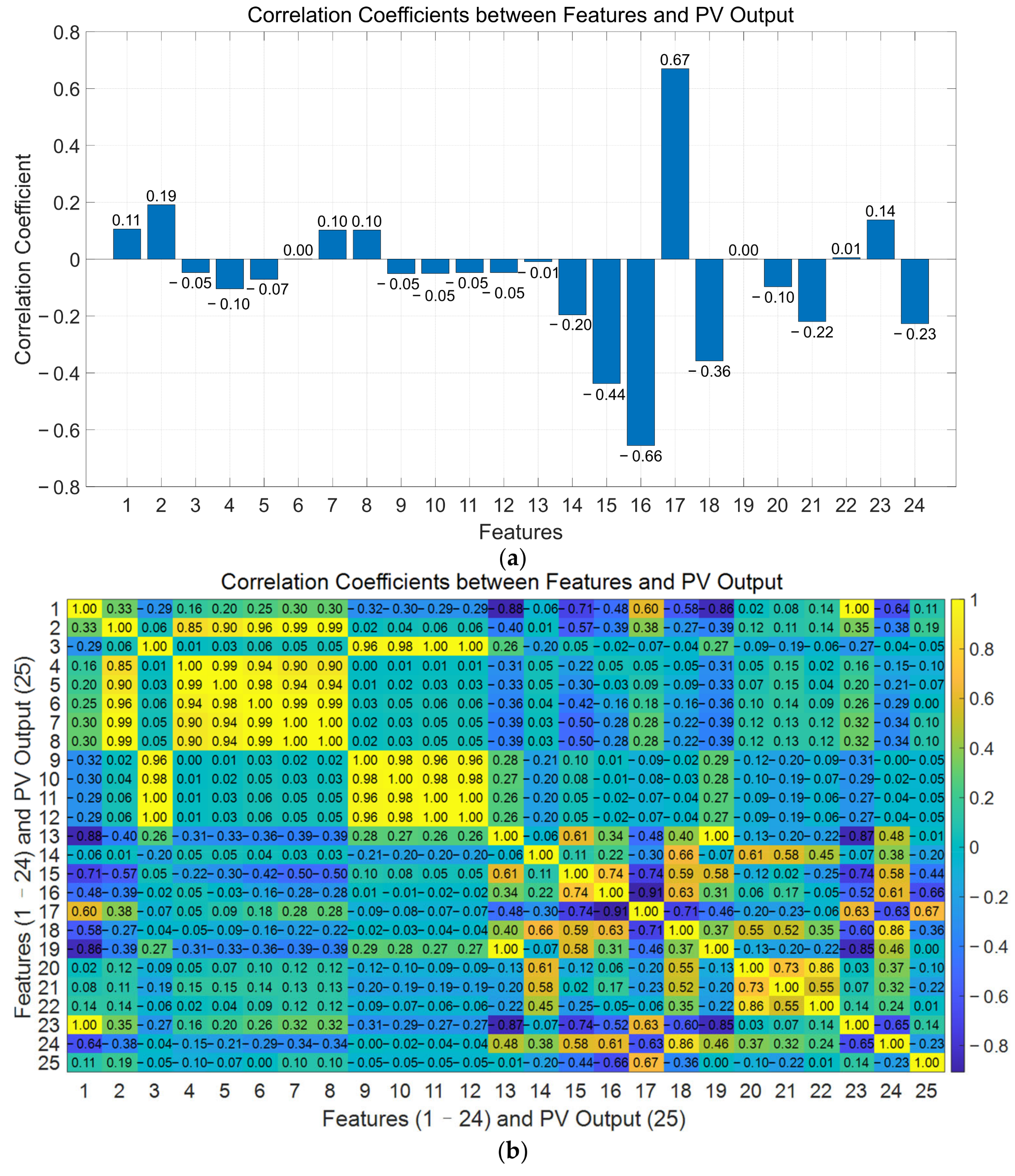
In addition, PV prediction includes multiple meteorological characteristics, such as solar radiation, temperature, wind speed, humidity, etc. PV power generation is significantly affected by meteorological conditions, and meteorological factors need to be comprehensively considered [22]. However, meteorological characteristics have different influences on PV output. Considering all meteorological characteristics can affect the prediction accuracy of the model [23]. Meteorological factors with low correlation should be analyzed and filtered to remove redundant features, thereby improving the prediction efficiency of the model.

Moreover, for multi-level PV clusters, which contain multiple PV stations, due to the change of weather conditions, considering that the power mutation of sub-regional (low-level) station output is larger than that of large-scale regional (high-level) station output, high-level output can reflect the change trend of the power generation data of a period of time and a region as a whole, and establish the trend reference with high-level output to improve the prediction performance of low-level output. It can help low-level stations predict power generation more accurately. In traditional PV prediction methods, only single-level predictions are considered, and the correlations among multi-level PV outputs are not taken into account. Therefore, effective information mining of the relationship between multi-level PV data is a necessary condition for enhancing the precision of PV power forecasting.

The instability of PV power generation poses challenges to the dispatching decisions of energy storage systems [24,25]. Deterministic prediction cannot provide sufficient information to predict the actual fluctuations in power generation. Therefore, probabilistic prediction is needed to quantify the uncertainty of PV prediction and help energy managers make more flexible decisions [26,27]. The parameter estimation method combining the analytical method, the simulated annealing method, and the derived model is used to analyze the characteristics of solar PV [28]. Parametric probabilistic prediction usually assumes that the data follow a specific distribution, such as the normal distribution and Poisson distribution. If the assumption does not hold true, the prediction result will be biased. Nonparametric probabilistic prediction effectively solves the problem of unknown distribution. A dual-branch deep learning quantile regression (QR) PV power prediction method is proposed to improve the prediction performance of the model [29]. PV power prediction is carried out by using the least squares SVM and KDE, which realizes the combination of deterministic prediction and uncertain prediction [30]. However, in the traditional KDE, a fixed bandwidth is used, and the bandwidth parameter controls the width of the kernel function, which lacks the flexible processing of each data point estimation, thereby affecting the smoothness and accuracy of the estimation. Therefore, through an effective KDE strategy, a relatively reasonable PI can be determined to ensure the reliability of the interval.

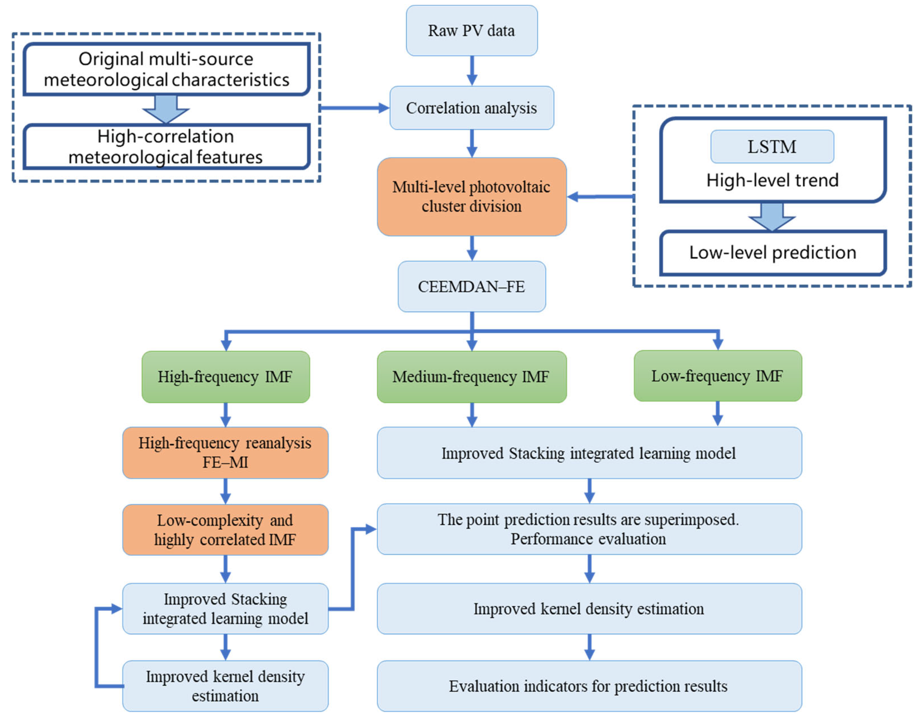
As a consequence, in this paper, a new short-term probabilistic forecasting model of PV power generation that utilizes multi-level adaptive dynamic integration is proposed. Firstly, the correlation between the high-level output and the low-level output within a PV region is analyzed to explore the potential relationship between multi-level PV outputs and the corresponding analysis results are introduced into the low-level output prediction model. Then, the PV data are decomposed by CEEMDAN and reconstructed with FE and MI (FE–MI). Then, the improved dual dynamic ensemble learning method is used to construct short-term PV power generation prediction models, and the high-frequency parts are analyzed and corrected. Finally, the adaptive KDE prediction error method is used to make interval predictions under different confidence levels to improve the overall performance of PIs. Compared with traditional PV forecasting models, the main contributions of this paper are as follows:

• The potential information on multi-level PV outputs is explored. The correlation between high-level PV output and low-level PV output is analyzed, and the prediction accuracy of low-level output is improved with the trend of high-level output;
• The proposed FE–MI method is used to reconstruct and analyze the PV data to extract the potential information, and the improved dual dynamic stacking model is used to make a deterministic prediction of PV power, thereby improving the accuracy of PV deterministic prediction;
• The proposed adaptive KDE method is used to correct the point prediction error of the high-frequency time series and is used to predict the probability of PV power, thereby obtaining a more reliable PI and quantifying the uncertainty of PV power.

The rest of this paper is organized as follows: Section 2 establishes theoretical methods and model structure; Section 3 introduces the dataset and evaluation metrics; in Section 4, the prediction results are given and analyzed; Section 5 summarizes the paper.

2. Methodology

2.1. Analysis of PV Data

According to the characteristics of multi-level PV data, the PV data are deeply mined. The method consists of CEEMDAN and FE–MI. These methods can be used to deeply mine multi-level PV data, extract potential useful information, and provide reliable data for subsequent model prediction.

2.1.1. CEEMDAN Method for PV Power

The correlation between the PV output of high-level stations and the PV output of low-level stations within the region is explored. Based on the high-level output analysis, the corresponding analysis results are introduced into the sample analysis stage of the low-level output prediction model; that is, the PV power generation and meteorological data of the low-level stations and the historical output of the high-level stations are clustered. The high-level output reflects the overall regional PV output change trend and improves judgment of the future change of low-level output.

The PV power of different clusters is decomposed by CEEMDAN. By using Gaussian white noise with a specific standard deviation, the CEEMDAN algorithm can extract each component and change trend of time series in an adaptive way, thereby reducing the mode aliasing defect of the empirical mode decomposition (EMD) algorithm and ensemble empirical mode decomposition algorithm. The detailed steps of CEEMDAN are as follows:

Step 1: For the original PV data $F(t)$, n Gaussian white noise sequences with an average of 0 are added to construct the sequence $F_i(t)$ to be decomposed.

$$F_i(t)=F(t)+{\lambda }_0{\omega }_i(t),i=1,2,3,\cdots ,n$$

(1)

where $t$ is the moment; ${\lambda }_0$ is the signal-to-noise ratio; and ${\omega }_i(t)$ is the white noise sequence added for the i time.

Step 2: The EMD algorithm is applied to each $F_i(t)$, and the first modal component $IM{F}_1(t)$ and the first unique residual component $R_1(t)$ are obtained.

$$IM{F}_1(t)={\displaystyle \frac{1}{n}}{\displaystyle \sum _{i=1}^n{E}_1(F_i(t))}$$

(2)

$$R_1(t)=F(t)-IM{F}_1(t)$$

(3)

where $E_1(\cdot )$ is the first component obtained by EMD decomposition.

Step 3: Noise is added to the residual component obtained after decomposition, and EMD is continued for decomposition.

$$IM{F}_k(t)={\displaystyle \frac{1}{n}}{\displaystyle \sum _{i=1}^n{E}_1[R_{k-1}(t)+{\lambda }_{k-1}{E}_{k-1}({\omega }_i(t))]},k=2,3,\cdots ,K$$

(4)

$$R_k(t)=R_{k-1}(t)-IM{F}_k(t)$$

(5)

where ${\lambda }_{k-1}$ is the signal-to-noise ratio of K − 1 white noise and $K$ is the number of intrinsic mode functions (IMFs) after decomposition.

Step 4: When the residual time series is a monotone function, the calculation is terminated. The original time series is decomposed into n modal components and the residual term R(t).

$$F(t)={\displaystyle \sum _{k=1}^{n}IM{F}_k(t)+R(t)}$$

(6)

2.1.2. FE–MI

FE is one of the criteria by which to measure the complexity of time series. It is an optimization method of approximate entropy and sample entropy. Compared with the other two methods, FE uses fuzzy membership function as the threshold criterion of entropy to ensure that it is more suitable for classifying and reassembling the components after frequency domain decomposition. The larger the FE, the more complex the time series. The specific steps for FE are as follows:

Step 1: For the time series $\{x(i),i=1,2,\cdots ,N\}$ of length $N$, dimension m is embedded to initialize the sequence and complete the phase space reconstruction, that is,

$$X(i)=\{x(i),x(i+1),\cdots ,x(i+m-1)\}-u(i)$$

(7)

$$u(i)={\displaystyle \frac{1}{m}}{\displaystyle \sum _{k=0}^{m-1}x(i+k)}$$

(8)

where $X(i)$ is the new sequence after reconstruction, $i=1,2,\cdots ,N-m+1$, and $u(i)$ is the mean of m continuous variables $x(i)$.

Step 2: The distance between two vectors $X(i)$ and $X(j)$ is defined as the maximum absolute value of the difference between the elements of the two vectors, and its expression is as follows:

$$d_{ij}^m=\max \{\left|[x(i+k)-u(i)]-[x(j+k)-u(i)]\right|\}$$

(9)

where $1\le i,j\le N-m+1$ and $i\ne j$.

Step 3: Fuzzy membership function is introduced to define the degree of similarity between vector $X(i)$ and $X(j)$, namely,

$$A_{ij}^m=\left\{\begin{array}{c}1,d_{ij}^m=0\\ \exp \left[-\ln 2{\left({\displaystyle \frac{d_{ij}^m}{r}}\right)}^2\right],d_{ij}^m>0\end{array}\right.$$

(10)

where $r$ is the similar tolerance parameter, defined as R times the standard deviation of the original one-dimensional time series, that is, $r=R\times \delta$, and where $\delta$ is the standard deviation of the original one-dimensional time series.

Step 4: The function $C_i^m(r)$ is defined, as shown in Equation (11). On this basis, the relation dimension ${\Phi }^m(r)$ in m dimension is obtained by Equation (12).

$$C_i^m(r)={\displaystyle \frac{1}{N-m}}{\displaystyle \sum _{j=1,j\ne i}^{N-m+1}{A}_{ij}^m}$$

(11)

$${\Phi }^m(r)={\displaystyle \frac{1}{N-m}}{\displaystyle \sum _{i=1}^{N-m+1}{C}_i^m(r)}$$

(12)

Step 5: The embedding dimension is increased by 1, and the above steps (1)~(4) are repeated for the m + 1 dimensional vector to obtain the following relation:

$${\Phi }^{m+1}(r)={\displaystyle \frac{1}{N-m}}{\displaystyle \sum _{i=1}^{N-m}{C}_i^{m+1}(r)}$$

(13)

Step 6: Equation (14) is used to calculate FE, and the classification and recombination of components are completed according to the proximity of entropy.

$$FE(m,r,N)=\ln {\Phi }^m(r)-\ln {\Phi }^{m+1}(r)$$

(14)

where $m$ is the embedding dimension parameter and $N$ is the length of the original time series.

The results of CEEMDAN decomposition are grouped and reconstructed according to FE for high, medium, and low frequency, and the high-frequency time series is decomposed in the frequency domain. Because the fluctuation of PV power is easily affected by weather, light intensity, and other factors, high-frequency IMF contains instantaneous fluctuations and instability, which can easily interfere with the prediction model. Therefore, it is necessary to further analyze the high-frequency components to extract useful information, retain the true change trend, reveal the short-term fluctuation laws affecting PV power, and mine the time-varying and nonstationary characteristics of high-frequency data to provide more accurate time series information for the model and further improve the accuracy of the prediction model.

MI is a measure of the interdependence between two random variables, which describes the amount of information contained in one variable about the other variable. Through MI, the correlation, dependence and information flow between variables can be obtained. For discrete random variables $X$ and $Y$, MI can be expressed as

$$I(X;Y)={\displaystyle \sum _{x\in X}{\displaystyle \sum _{y\in Y}p(x,y)\log \frac{p(x,y)}{p(x)p(y)}}}$$

(15)

where $p(x,y)$ is the joint probability distribution function of $X$ and $Y$, and $p(x)$ and $p(y)$ are the edge probability distribution functions of $X$ and $Y$, respectively.

The FE can measure the complexity of the time series, and a higher FE usually means a higher complexity of the time series and a more chaotic structure. MI measures the correlation between two time series, and the greater the MI, the stronger the correlation. By selecting the time series with the smallest ratio of FE divided by MI, the mode containing both low complexity and low redundancy is found. Therefore, after frequency domain decomposition of high-frequency time data, the selection of the IMF with the smallest FE/MI ratio can provide cleaner, more accurate, and more representative data for subsequent forecasts. This not only helps to improve the prediction accuracy, training efficiency, and generalization ability of the model, but also reduces the negative impact of noise and redundant information on the prediction results.

2.2. Improved Dual Dynamic Stacked Ensemble Learning Model

Ensemble learning improves the overall prediction performance by combining the prediction results of multiple learning models, that is, combining multiple weak learners into one strong learner, thereby enhancing the accuracy, robustness, and generalization ability of the model. By taking advantage of the strengths of multiple models, the deviation and variance problems that occur in a single model can be effectively reduced, and the accuracy and stability of the final prediction can be improved. Ensemble learning has the following main forms: bootstrap aggregating (Bagging), Boosting, and Stacking. Bagging uses bootstrap sampling to improve stability. Boosting improves accuracy by adjusting the weights of training samples. However, the base learners of the above two are usually the same. Stacking combines multiple different types of base learners together, and each base learner generates a prediction result. Then, another model is used to conduct secondary learning on the prediction results of these base learners to generate the final prediction. Stacking is more flexible due to integrating multiple different types of models and is suitable for a wide variety of learners and datasets. It can capture more diverse features, thereby improving the prediction performance. Stacking usually adopts a double-layer structure for model fusion. The first layer is the base learner layer: Multiple different models are trained on the raw data to output predicted values. The second layer is the meta-learner layer: The prediction results of the base learner are taken as input features, and the meta-learning model is set for secondary training to generate the final prediction results. The Stacking model framework is shown in Figure 1.

Stacking combines different base learners to give full play to the different characteristics and advantages of the base model, thereby improving the performance of the overall model. However, in traditional Stacking, the base learner is usually fixed and remains unchanged throughout the training process, unable to cope with different data distributions and PV prediction scenarios, and lacks adaptability. Therefore, it is necessary to improve the Stacking model. A new dual dynamic adaptive Stacking model is proposed in this paper. For a single dataset, multiple training sets can be dynamically divided, and PV prediction can be adaptively carried out in the dual dynamic mode of dynamic datasets and dynamic models. Dynamically adjusted Stacking can dynamically select and adjust datasets and base learners according to the characteristics and changes of the data. This approach can adaptively adjust according to the current training environment and continuously optimize the selection and combination of base learners, thereby improving the overall model performance and having a stronger generalization ability. The improved dual dynamic stacked ensemble learning model is shown in Figure 2.

A new dual dynamic stacked ensemble learning method for PV prediction based on the adaptive dual dynamic mode of data and models is proposed in this paper. The multiple datasets are dynamically divided, and the three optimal models are selected from the five pre-set basic models for model training. By continuously optimizing the selection and combination of data and base learners, the adaptability and generalization ability of the model are improved. In this paper, CNN, backpropagation (BP) neural networks, K-nearest neighbor (KNN), SVM, and RF are pre-set as the basic learners, and LSTM is set as the meta-learner. These base learners perform well on small datasets and have obvious advantages in computational efficiency and overfitting control, which can achieve better overall prediction results. LSTM is suitable for processing sequential data, capable of capturing the long-term dependencies in the prediction results of base learners, and can analyze the data distribution of each base learner with its unique memory mechanism.

2.3. Improved KDE

Nonparametric estimation is different from traditional parametric estimation in that it does not assume the distribution form of the data. Nonparametric estimation is used when the distribution of the data is not explicitly assumed, or the distribution of the data may be unknown or difficult to determine. KDE in nonparametric estimation is used to estimate the probability density function of a random variable, which approximates the true probability distribution by distributing data points around each point of the sample data to build a smooth curve. The principle is to specify a neighborhood range with a certain bandwidth for the target point, count the number of elements in the neighborhood, and calculate the average density. The KDE equation is as follows:

$$f(x)={\displaystyle \frac{1}{Nd}}{\displaystyle \sum _{i=1}^{N}K\left(\frac{x-{\beta }_i}{d}\right)}$$

(16)

where $N$ is the total number of sample points; $x$ is the target sample point; ${\beta }_i$ is the sample value of point $i$; $d$ is the window width; and $K(\cdot )$ is a kernel function; common kernel functions include Gaussian kernel, uniform kernel, Epanechnikov kernel, etc. In this paper, the Gaussian kernel function is selected, and the expression of $f\left(x\right)$ becomes

$$f(x)={\displaystyle \frac{1}{\sqrt{2\pi }}}{\displaystyle \frac{1}{Nd}}{\displaystyle \sum _{i=1}^N\exp \left[-\frac{1}{2}{\left(\frac{x-{\beta }_i}{d}\right)}^2\right]}$$

(17)

The choice of bandwidth in KDE is important because it directly affects the quality of the final estimated probability density function. The bandwidth determines the width of the kernel function, which in turn affects the smoothness of the estimation. Excessive bandwidth leads to excessive smoothing, ignoring detailed features in the data; on the other hand, too small a bandwidth easily leads to introducing noise, making the estimation unstable and not smooth.

For the characteristics of single-peak power and multi-peak power, the optimal bandwidth is determined by the standard deviation and standard quartile distance of the power prediction sample. The equation for calculating bandwidth $d$ by the thumb method of the KDE model based on the Gaussian kernel function is

$$d=1.06\min \left\{S,{\displaystyle \frac{Q}{1.34}}\right\}{N}^{-{\displaystyle \frac{1}{5}}}$$

(18)

where $N$ is the number of sample points; $S$ is the sample standard deviation; and $Q$ is the standard quartile of the data.

The improved KDE method not only performs probabilistic prediction analysis on the deterministic prediction results of multi-level decomposition of PV power, but also corrects the error of deterministic prediction results of high-frequency time series after decomposition and reconstruction; that is, the point prediction results are corrected according to the PIs of probabilistic prediction. The correction equation is shown as follows:

$$corr=y_i+\left({\widehat{y}}_{i0}-y_{i0}\right)\cdot \left(q_{\overline{\alpha 0}}-q_{\underset{¯}{\alpha 0}}\right)$$

(19)

where $y_i$ is the current predicted value; ${\widehat{y}}_{i0}$ and $y_{i0}$ are, respectively, the average true values and average predicted values at the same time over a known 5 days under similar weather conditions; and $q_{\overline{\alpha 0}}$ and $q_{\underset{¯}{\alpha 0}}$ are, respectively, the upper and lower boundaries of the mean division of the PIs at the same time over a known 5 days under similar weather conditions.

2.4. The Proposed Forecasting Model

The flow chart of the proposed model is shown in Figure 3. First, the correlation analysis of PV data and meteorological data is carried out to remove unnecessary meteorological characteristics. Then, the PV data for high-level and low-level stations are divided into clusters, and the output prediction of low-level stations is optimized according to the output trend of high-level stations. The output trend of high-level stations is the predicted value of the actual PV power, which is predicted by LSTM. The correlation between the high and low levels of output within the PV area is analyzed, and the corresponding analysis results are introduced into the low-level output prediction model. Then, the PV data are decomposed by CEEMDAN, and the high-frequency IMF, medium-frequency IMF, and low-frequency IMF are divided according to FE. Because the fluctuation of PV power is easily affected by weather, light intensity, and other factors, high-frequency IMF contains instantaneous fluctuations and instability, which can easily interfere with the prediction model. Therefore, further analysis of the high-frequency components is needed to extract useful information. The high-frequency time series is decomposed again. The high-frequency IMF is reconstructed and analyzed based on FE and MI entropy. The components with low complexity and high correlation to the original high-frequency time series are extracted as the basic analytical quantities of the high-frequency time series; that is, the decomposition quantities with low complexity and certain patterns are further mined from the high-frequency IMF for point prediction analysis. Medium-frequency IMF and low-frequency IMF indicate the long-term trend of PV power, including relatively stable and regular changes, which can be directly input into the prediction model to improve the prediction efficiency and accuracy of the model. Then, the decomposed multi-level data are input into the improved Stacking for training to obtain the deterministic prediction values, and the improved KDE method is used to optimize the prediction results of the filtered high-frequency time series (high-frequency reanalysis components). Finally, the uncertainty of PV prediction is quantified by using adaptive KDE to make probabilistic prediction of the overall forecast output through the deterministic predicted value and prediction error.

3. Materials and Metrics

3.1. Description of Dataset

Several PV power plants with an installed capacity of 30 MW in China are used for validation in this paper, among which the installed capacity of the high-level PV station is 6 MW, and the installed capacity of the low-level PV station is 300 kW, and the high-level PV power station includes multiple low-level PV power stations. It is a 24 h all-weather dataset with a data resolution of 15 min. The meteorological data consist of 24 weather variables, including air temperature, wind direction, wind speed, air pressure, cloud cover, heat flux, heat radiation, precipitation, humidity, and other meteorological forecast information. The time scale for short-term PV prediction is the next 1 to 3 days. The input of the prediction model is meteorological characteristics, and the output is PV power. In this paper, datasets from January 1 to June 30 are used to forecast the actual PV power for the next 3 days. Since PV power at night is almost 0, the prediction is of little significance, so the periods without power generation in the early morning and at night are excluded during model training. The dataset is divided into a training set and a test set, with a ratio of 8:2. The sample sizes of the training set and the test set are 3371 and 843, respectively.

3.2. Evaluation Metrics

The error index is a unified standard for measuring prediction accuracy. Five different evaluation metrics, namely, root mean square error (RMSE), mean absolute error (MAE), mean absolute percentage error (MAPE), coefficient of determination (R²), and accuracy rate, are used in this paper to assess the discrepancy between forecasted and actual values and quantify the deterministic performance of the prediction model. The calculation equations for each metric are as follows:

$$RMSE=\sqrt{{\displaystyle \frac{1}{N}}{\displaystyle \sum _{i=1}^N{\left(\frac{{\widehat{y}}_i-y_i}{c_i}\right)}^2}}$$

(20)

$$MAE={\displaystyle \frac{1}{N}}{\displaystyle \sum _{i=1}^N\left|\frac{{\widehat{y}}_i-y_i}{c_i}\right|}$$

(21)

$$MAPE={\displaystyle \frac{1}{N}}{\displaystyle \sum _{i=1}^N\left|\frac{{\widehat{y}}_i-y_i}{y_i}\right|}\times 100\%$$

(22)

$$R^2=1-{\displaystyle \sum _{i=1}^N{\left({\widehat{y}}_i-y_i\right)}^2}/{\displaystyle \sum _{i=1}^N{\left({\overline{y}}_i-y_i\right)}^2}$$

(23)

$$Accuracy=1-RMSE$$

(24)

where $N$ is the number of predicted samples; $y_i$ is the predicted value; ${\widehat{y}}_i$ is the true value; ${\overline{y}}_i$ is the mean of the true values; and $c_i$ is the installed capacity.

For probabilistic prediction, PI coverage probability (PICP), PI normalized average width (PINAW), and interval score (IS) are used as evaluation indicators in this paper. The evaluations include reliability and overall performance, which are given in Equations (25)–(30).

$$PICP={\displaystyle \frac{1}{T_p}}{\displaystyle \sum _{i=1}^{T_p}{\eta }_i}$$

(25)

$${\eta }_i=\left\{\begin{array}{c}1\hspace{0.33em}\hspace{0.33em}\hspace{0.33em}{t}_i\in I_{\alpha }\\ 0\hspace{0.33em}\hspace{0.33em}\hspace{0.33em}{t}_i\notin I_{\alpha }\end{array}\right.$$

(26)

$$A{W}^{\alpha }={\displaystyle \sum _{i=1}^{T_p}W(x_i)}$$

(27)

$$W(x_i)=q_{\overline{\alpha }}(x_i)-q_{\underset{\_}{\alpha }}(x_i)$$

(28)

$$S_{\alpha }(x_i)=\left\{\begin{array}{l}-2(1-\alpha )W(x_i)-4(q_{\underset{\_}{\alpha }}(x_i)-t_i)\hspace{0.33em}\hspace{0.33em}\hspace{0.33em}{t}_i<q_{\underset{\_}{\alpha }}(x_i)\\ -2(1-\alpha )W(x_i)\hspace{0.33em}\hspace{0.33em}\hspace{0.33em}\hspace{0.33em}\hspace{0.33em}\hspace{0.33em}\hspace{0.33em}\hspace{0.33em}\hspace{0.33em}\hspace{0.33em}\hspace{0.33em}\hspace{0.33em}\hspace{0.33em}\hspace{0.33em}\hspace{0.33em}\hspace{0.33em} t_i\in I_{\alpha }(x_i)\\ -2(1-\alpha )W(x_i)-4(t_i-q_{\overline{\alpha }}(x_i))\hspace{0.33em}\hspace{0.33em}\hspace{0.33em}{t}_i>q_{\overline{\alpha }}(x_i)\end{array}\right.$$

(29)

$$I{S}_{\alpha }={\displaystyle \frac{1}{T_p}}{\displaystyle \sum _{i=1}^{T_p}{S}_{\alpha }(x_i)}$$

(30)

where $T_p$ is the number of predicted samples; ${\eta }_i$ is the Boolean quantity; $t_i$ is the predicted value; I_a is the forecast interval; $A{W}^{\alpha }$ is the width of the PI; $W\left(x_i\right)$ is the width of each PI; $q_{\overline{\alpha }}$ is the upper boundary; $q_{\underset{¯}{\alpha }}$ is the lower boundary; $S_{\alpha }\left(x_i\right)$ is the bandwidth deviation of the PI of the i iteration; and $\alpha$ is the quantile.

4. Case Studies

4.1. Multi-Level PV Data Analysis Results

The validity of meteorological characteristics should be taken into account in the prediction of PV power generation capacity. Some meteorological characteristics are dispensable for the prediction effect. Therefore, it is necessary to analyze the meteorological characteristics, remove the features with low correlation, and avoid affecting the prediction performance. In this paper, the Spearman [31] correlation coefficient is used to calculate the correlation between PV power and various meteorological characteristics, and the meteorological characteristics with higher correlations are obtained for subsequent analysis. Figure 4 shows the calculation results of the correlation coefficient.

Figure 4a shows a bar chart of the correlation between 24 meteorological features and PV power. Figure 4b shows the heat map of the correlations between 24 meteorological features and PV power, respectively. According to Spearman’s evaluation criterion, meteorological and geographical features with an absolute value of the correlation coefficient of 0.3 or above should be selected. Therefore, in the PV power prediction of this paper, sensible heat flux, latent heat flux, short-wave radiation, and long-wave radiation are taken as meteorological characteristics data.

By exploring the correlation between the high-level output and the low-level output within the region, the high-level output reflects the change trend of the overall PV output in the region so as to improve the judgment of the future change of the low-level output. Combining the historical data of low-level and high-level stations and the predicted output of the high-level stations, the training sample is optimized. In this paper, K-means [32] is used for clustering, the power output of the high-level stations is taken as one of the clustering input variables, and the PV output of the low-level stations is taken as the forecast object. The clustering results are shown in Figure 5.

Since the PV data at night are almost 0, it is of little significance to predict it. The PV data from 6:00 to 18:00 are selected for clustering in this paper. The optimal number of clusters is selected by comparing the performance of model prediction under different numbers of clusters. As can be seen from Figure 5, the PV data of high-level and low-level stations are clustered into four categories. Figure 5a shows the clustering situation of each sampling point, and Figure 5b shows the clustering situation of 49 samples per day. By analyzing the correlation between high-level PV power and low-level PV power, the trend of high-level PV power is used to optimize the prediction of low-level PV power. LSTM is used to predict the high-level PV power, and the input of the low-level PV output prediction model, that is, meteorological characteristics, and the prediction results of high-level PV power are taken as analysis samples. The clustering of PV data is carried out to improve the accuracy of the samples used in the prediction model, achieve multi-level correlation analysis, and optimize the judgment of the prediction model on the overall output and the change trend of weather processes in the region.

In this paper, the CEEMDAN algorithm is adopted to decompose the PV data of each cluster after clustering to obtain multiple components, and the high-frequency, medium-frequency, and low-frequency IMF are obtained through EF. For the high-frequency IMF, variational mode decomposition [33] is adopted for further decomposition, and the high-frequency reanalysis components with low complexity and high correlation are selected through EF–MI. Figure 6 shows the decomposition results of CEEMDAN and the high-frequency, medium-frequency, and low-frequency IMF components obtained after the final optimization.

4.2. Analysis of Deterministic Prediction Results

The training set is dynamically divided into three training sets, and the proportion of each training set is half of the original training set, that is, to make each training set contain similar data as much as possible to avoid the contingency of model training. The number of samples in each of the three training sets of cluster I is 3371. The parameter configurations of each model in this paper are shown in

Table 2. Configuration of model parameters.

Model	CNN	BP	KNN	SVM	RF	LSTM	ELM
Optimizer	Adam	Levenberg–Marquardt	-	SMO	Bagging	Adam	-
Convolutional kernels	10	-	-	-	-	-	-
Kernel	-	-	-	RBF	-	-	-
Trees	-	-	-	-	50	-	-
Neighbors	-	-	5	-	-	-	-
Hidden units	-	10	-	-	-	10	25
Max iterations	100	100	-	-	-	100	-
Learning rate	0.01	0.01	-	-	-	0.01	-

.

The pre-set CNN, BP, KNN, SVM, and RF are trained, respectively, on three training sets. Each model is independent and does not interfere with any other.

Table 3. Evaluation index of base learners in each training set.

Training Set	Prediction Model	RMSE/MW	MAE/MW	MAPE/%	Accuracy/%
1	CNN	0.2377	0.1686	1.70	76.23
	BP	0.2324	0.1687	1.67	76.76
	KNN	0.3044	0.2114	2.14	69.56
	SVM	0.1543	0.1082	0.80	84.57
	RF	0.2278	0.1595	1.62	77.22
2	CNN	0.2852	0.2235	1.52	71.48
	BP	0.2491	0.1979	1.27	75.09
	KNN	0.3655	0.2857	2.02	63.45
	SVM	0.1887	0.1342	0.78	81.13
	RF	0.2792	0.2178	1.48	72.08
3	CNN	0.2007	0.1570	0.88	79.93
	BP	0.2000	0.1584	0.79	80.00
	KNN	0.2715	0.1896	1.36	72.85
	SVM	0.1816	0.1248	0.76	81.84
	RF	0.1911	0.1475	0.83	80.89

presents the performance indicators of the five models on the three training sets.

It can be observed in Table 3 that the prediction performance of the five models is the best in the third training set. Therefore, the third training set is selected as the optimal training set. In the third training set, the prediction effects of CNN and KNN are poor. Therefore, CNN and KNN are abandoned, and BP, SVM, and RF are selected as the chosen base learners.

After determining the optimal training set and the Stacking base learner, the integrated learning model of high-frequency, medium-frequency, and low-frequency IMF is trained, respectively. Finally, the prediction results are superimposed, and the prediction errors are analyzed. For high-frequency IMF, adaptive KDE is used to make probabilistic predictions, and the prediction results are determined by ensemble learning of PI correction for high-frequency IMF. In order to prove the advantages of the Stacking ensemble learning approach for short-term PV power forecasting proposed in this paper, the proposed approach is evaluated against the single machine learning methods LSTM and ELM and compared with the traditional Stacking model, and the parameter settings in the comparison model are consistent with the model established in this paper. The traditional Stacking model that uses the data processing method in this paper is represented by ICEEMDAN–Stacking, and the proposed model is represented by ICEEMDAN–I-Stacking. Figure 7 shows the prediction results of cluster I dataset three days ahead, and the evaluation indicators are shown in

Table 4. Evaluation indicators for forecast results of cluster I three days ahead.

Prediction Model	RMSE/MW	MAE/MW	MAPE/%	R2	Accuracy/%	Training Time/s
LSTM	0.2052	0.1711	26.46	0.4152	79.48	35.56
ELM	0.1959	0.1626	26.07	0.4672	80.41	0.12
Stacking	0.1627	0.1216	20.86	0.6324	83.73	8.34
CEEMDAN–Stacking	0.1722	0.1317	22.18	0.5882	82.78	18.48
ICEEMDAN–Stacking	0.1553	0.1237	20.10	0.6651	84.47	19.99
ICEEMDAN–I-Stacking	0.1307	0.0999	16.26	0.7628	86.93	78.73

.

The predicted results of cluster II dataset three days ahead are shown in Figure 8, and

Table 5. Evaluation indicators for forecast results of cluster II three days ahead.

Prediction Model	RMSE/MW	MAE/MW	MAPE/%	R2	Accuracy/%	Training Time/s
LSTM	0.1731	0.1436	22.40	0.6116	82.69	39.83
ELM	0.1934	0.1596	25.18	0.5150	80.66	0.12
Stacking	0.1409	0.1041	18.95	0.7426	85.91	9.32
CEEMDAN–Stacking	0.1606	0.1201	21.41	0.6658	83.94	21.76
ICEEMDAN–Stacking	0.1396	0.1078	18.79	0.7473	86.04	25.24
ICEEMDAN–I-Stacking	0.1228	0.0915	15.97	0.8044	87.72	74.75

shows the evaluation indicators.

Figure 7 and Figure 8, respectively, show the prediction result curves of each model in cluster I and cluster II three days ahead. It can be seen from the comparison of the three-day-ahead prediction errors for cluster I in Table 4 and for cluster II in Table 5 that the prediction accuracy of individual LSTM and ELM models is relatively low. The traditional Stacking model utilizes the advantages of multiple base learners to improve the prediction performance. Although PV data are analyzed in the CEEMDAN–Stacking model, the prediction accuracy is reduced due to insufficient mining. The ICEEMDAN–Stacking model further improves the prediction accuracy through sufficient data mining, but the prediction performance of this model is poor compared with the proposed ICEEMDAN–I-Stacking. The proposed I-Stacking can further optimize the integrated learning structure and obtain better prediction accuracy. The proposed model further optimizes the prediction accuracy by correcting the deterministic prediction results through the PIs, and is superior to other comparison models in each evaluation index. Compared to other models, the RMSE of the proposed method in the cluster I dataset decreased by 36.31%, 33.28%, 19.67%, 24.10%, and 15.84%, respectively, and the MAE decreased by 41.61%, 38.56%, 17.85%, 24.15%, and 19.24%, respectively. Compared to other models, the RMSE of the proposed method in the cluster II dataset decreased by 29.06%, 36.50%, 12.85%, 23.54%, and 12.03%, respectively, and the MAE decreased by 36.28%, 42.67%, 12.10%, 23.81%, and 15.12%, respectively. A personal computer configured with an Intel(R) Core(TM) i7-9750H CPU @ 2.60 GHz and 16.0 GB RAM is used for computing. The training time of the proposed model is less than 100 s, and the testing time is less than 1 s. The calculation efficiency can meet the practical application requirements of short-term PV power prediction. Among all the models, the predicted results have the highest fitting degree with the true values, and the accuracy is also the highest, indicating that the proposed method can effectively improve the accuracy of the three-day-ahead PV power prediction model.

To further verify the superiority of the proposed deterministic prediction model method, an example of day-ahead PV prediction is provided for illustration.

Table 6. Evaluation indicators of the day-ahead PV power prediction result.

Prediction Model	RMSE/MW	MAE/MW	MAPE/%	R2	Accuracy/%	Training Time/s
LSTM	0.2164	0.1838	31.15	0.4474	78.36	52.77
ELM	0.2246	0.1850	31.31	0.4049	77.54	0.19
Stacking	0.1601	0.1168	17.22	0.6976	83.99	15.66
CEEMDAN–Stacking	0.1548	0.1123	16.80	0.7173	84.52	19.71
ICEEMDAN–Stacking	0.1551	0.1172	17.69	0.7163	84.49	17.55
ICEEMDAN–I-Stacking	0.1276	0.0888	12.50	0.8081	87.24	66.59

shows the performance indicators of each prediction model one day ahead.

It can be seen from the comparison of prediction errors in Table 6 that in the PV power prediction one day ahead, the prediction accuracy of both the LSTM and ELM models is relatively low. The traditional Stacking model and CEEMDAN–Stacking model can improve the prediction performance. The ICEEMDAN–Stacking model improves the prediction accuracy through sufficient data mining, but it is not as good as the proposed ICEEMDAN–I-Stacking model. The proposed method can further optimize the prediction accuracy and outperforms other comparison models in all evaluation indicators. Among all the models, the proposed method has the highest degree of fitting between the predicted results and the true values, as well as the highest accuracy. The training time of the proposed model is less than 100 s, and the testing time is less than 1 s. The calculation efficiency can meet the actual requirements. Therefore, the proposed method can effectively improve the accuracy of the day-ahead PV power generation prediction model.

4.3. Analysis of Probabilistic Prediction Results

The proposed deterministic prediction method improves the accuracy of short-term PV prediction, but it does not reflect the reliability and uncertainty of prediction. Probabilistic prediction can provide distribution information of predicted results, which helps decision makers to make more intelligent decisions and reduce risks. The probabilistic prediction results of the proposed improved KDE for the three-day-ahead PV power are shown in Figure 9 below.

Figure 9 shows that for cluster I and cluster II datasets, the three-day-ahead PV prediction has high reliability at both 90% PI normalized confidence (PINC) and 95% PINC, and the average width of PIs is narrow and the clarity is high. Therefore, the PI of the proposed approach has high reliability and good sharpness.

In order to verify the effectiveness of the probabilistic prediction method for improved KDE proposed in this paper, the proposed method is compared with traditional Gaussian, QR, Bootstrap, and KDE, and data with a PINC of 90% are selected for comparison. The proposed adaptive dynamic KDE method is represented by AKDE. The comparison results of error indicators three days ahead are shown in

Table 7. Evaluation indicators for probabilistic prediction results three days ahead.

Dataset	Prediction Model	PICP/%	PINAW	IS
Cluster I	Gaussian	90.5101	11.6663	−3.3836
	QR	91.2218	12.1024	−3.3750
	Bootstrap	90.2728	13.1122	−3.8348
	KDE	90.9846	13.1025	−3.7638
	AKDE	91.9502	11.4966	−2.9702
Cluster II	Gaussian	90.6696	10.5198	−3.0555
	QR	91.6575	11.1686	−3.0618
	Bootstrap	90.5598	11.1644	−3.3623
	KDE	90.3403	11.2027	−3.4043
	AKDE	91.7311	10.1919	−2.8265

.

For probabilistic prediction, the higher the PICP and IS, and the smaller the PINAW, the better the prediction indicators. Therefore, as shown in the three-day-ahead probabilistic prediction results of Table 7, compared with Gaussian, QR, Bootstrap, and KDE methods, the overall performance of the proposed method is the best: PICP of cluster I is increased by 1.44%, 0.73%, 1.68%, and 0.97%, respectively, while PINAW is decreased by 1.45%, 5.01%, 12.32%, and 12.26%, respectively. PICP of cluster II is increased by 1.06%, 0.07%, 1.17%, and 1.39%, respectively, while PINAW is decreased by 3.12%, 8.75%, 8.71%, and 9.02%, respectively. The IS of the proposed AKDE method is also the highest in the two clusters. Therefore, the results show that under different datasets, compared with traditional probabilistic prediction methods, the proposed method overall has better reliability and prediction performance in three-day-ahead PV probabilistic prediction.

To further verify the superiority of the proposed probabilistic prediction model method, an example of day-ahead PV prediction is provided for illustration, and the data with a PINC of 90% are selected for comparison.

Table 8. Evaluation indicators for probabilistic prediction results one day ahead.

Prediction Model	PICP/%	PINAW	IS
Gaussian	90.6036	11.6845	−3.6911
QR	90.8994	11.8994	−3.6482
Bootstrap	89.7929	11.6996	−3.8475
KDE	90.5325	11.6355	−3.7656
AKDE	91.1467	10.9941	−3.4379

shows the evaluation indicators of each probabilistic prediction model one day ahead.

As shown in the day-ahead probabilistic prediction results of Table 8, compared with Gaussian, QR, Bootstrap, and KDE methods, the overall performance of the proposed method is the best. The PICP and IS of the proposed AKDE method are the highest, and the PINAW is the lowest. Therefore, the proposed method has better reliability and prediction performance in day-ahead PV probabilistic prediction.

5. Conclusions

In this paper, an improved PV short-term power prediction method based on multi-level adaptive dynamic integration is proposed to solve the problems of deterministic and probabilistic predictions of PV power generation time series. The theory that the trend of high-level output optimizes the prediction of low-level output has been applied, and the main environmental factors that constrain PV power generation have been fully considered in this method. The main conclusions are as follows:

• Based on the relationship between multi-level PV data, considering that the power mutability of low-level output is larger than that of high-level output, the high-level output reflects the change trend of power generation and improves the prediction performance of low-level output;
• Through the proposed FE–MI method, multi-layer reconstruction analysis of PV data is carried out to extract the potential information for PV power generation, improve the reliability of data input, and improve the accuracy of PV prediction;
• A new dynamic adaptive Stacking integration method is proposed. Adaptive PV prediction is carried out through the dual dynamic mode of data and models to enhance the adaptability of the model and improve its generalization ability;
• A new adaptive window width optimization strategy is proposed to establish PIs with high overall performance. The proposed method enhances the quality of prediction error analysis by comprehensively considering the reliability and overall performance of PIs.

References

1. Aghajari, H.A.; Niknam, T.; Shasadeghi, M.; Sharifhosseini, S.M.; Taabodi, M.H.; Sheybani, E.; Javidi, G.; Pourbehzadi, M. Analyzing complexities of integrating Renewable Energy Sources into Smart Grid: A comprehensive review. Appl. Energy 2025, 383, 125317. [Google Scholar] [CrossRef]
2. Wu, D.; Fu, Y.; Li, M.; Ouyang, L. A Combined Compensation Strategy for Steady-State Performance Improvement of Proportional-Proportional-Delay Controller. IET Power Electron. 2025, 18, e70022. [Google Scholar] [CrossRef]
3. Husein, S.M.; Gago, E.J.; Hasan, B.; Pegalajar, M.C. Towards energy efficiency: A comprehensive review of deep learning-based photovoltaic power forecasting strategies. Heliyon 2024, 10, e33419. [Google Scholar] [CrossRef] [PubMed]
4. Wu, D.; Zhi, Q.; Li, M.; Zhao, Y.; Tian, H. Control strategy for L-type grid-connected inverters under ultra-weak grid conditions. J. Power Electron. 2025, 1–12. [Google Scholar] [CrossRef]
5. Zhou, Y.; Wei, F.; Kuang, K.; Mahfoud, R.J. Research on a deep ensemble learning model for the ultra-short-term probabilistic prediction of wind power. Electronics 2024, 13, 475. [Google Scholar] [CrossRef]
6. Yang, M.; Guo, Y.; Fan, F. Ultra-short-term prediction of wind farm cluster power based on embedded graph structure learning with spatiotemporal information gain. IEEE Trans. Sustain. Energy 2025, 16, 308–322. [Google Scholar] [CrossRef]
7. Yang, M.; Han, C.; Zhang, W.; Wang, B. A short-term power prediction method for wind farm cluster based on the fusion of multi-source spatiotemporal feature information. Energy 2024, 294, 130770. [Google Scholar] [CrossRef]
8. Li, M.; Tian, Y.; Zhang, H.; Zhang, N. The source-load-storage coordination and optimal dispatch from the high proportion of distributed photovoltaic connected to power grids. J. Eng. Res. 2024, 12, 421–432. [Google Scholar] [CrossRef]
9. Yang, M.; Shen, X.; Huang, D.; Su, X. Fluctuation classification and feature factor extraction to forecast very short-term photovoltaic output powers. CSEE J. Power Energy Syst. 2025, 11, 661–670. [Google Scholar]
10. Fu, X. Statistical machine learning model for capacitor planning considering uncertainties in photovoltaic power. Prot. Control Mod. Power Syst. 2022, 7, 5. [Google Scholar] [CrossRef]
11. Yang, M.; Jiang, Y.; Xu, C.; Wang, B.; Wang, Z.; Su, X. Day-ahead wind farm cluster power prediction based on trend categorization and spatial information integration model. Appl. Energy 2025, 388, 125580. [Google Scholar] [CrossRef]
12. Dudáš, A.; Udristioiu, M.T.; Alkharusi, T.; Yildizhan, H.; Sampath, S.K. Examining effects of air pollution on photovoltaic systems via interpretable random forest model. Renew. Energy 2024, 232, 121066. [Google Scholar] [CrossRef]
13. Liu, H.; Cai, C.; Li, P.; Tang, C.; Zhao, M.; Zheng, X.; Li, Y.; Zhao, Y.; Liu, C.; Liu, C. Hybrid prediction method for solar photovoltaic power generation using normal cloud parrot optimization algorithm integrated with extreme learning machine. Sci. Rep. 2025, 15, 6491. [Google Scholar] [CrossRef] [PubMed]
14. Zhu, R.; Li, T.; Tang, B. Research on short-term photovoltaic power generation forecasting model based on multi-strategy improved squirrel search algorithm and support vector machine. Sci. Rep. 2024, 14, 14348. [Google Scholar] [CrossRef] [PubMed]
15. He, Q.; Zhao, M.; Li, S.; Li, X.; Wang, Z. Machine Learning Prediction of Photovoltaic Hydrogen Production Capacity Using Long Short-Term Memory Model. Energies 2025, 18, 543. [Google Scholar] [CrossRef]
16. Srikanth, D.; Sukumar, G.D.; Sobhan, P.V. A convolutional neural network based energy management system for photovoltaic/battery systems in microgrid using enhanced coati optimization approach. J. Energy Storage 2025, 119, 116252. [Google Scholar] [CrossRef]
17. Babalhavaeji, A.; Radmanesh, M.; Jalili, M.; González, S.A. Photovoltaic generation forecasting using convolutional and recurrent neural networks. Energy Rep. 2023, 9, 119–123. [Google Scholar] [CrossRef]
18. Sabri, M.; El Hassouni, M. Photovoltaic power forecasting with a long short-term memory autoencoder networks. Soft Comput. 2023, 27, 10533–10553. [Google Scholar] [CrossRef]
19. Sarmas, E.; Spiliotis, E.; Stamatopoulos, E.; Marinakis, V.; Doukas, H. Short-term photovoltaic power forecasting using meta-learning and numerical weather prediction independent Long Short-Term Memory models. Renew. Energy 2023, 216, 118997. [Google Scholar] [CrossRef]
20. Khan, W.; Walker, S.; Zeiler, W. Improved solar photovoltaic energy generation forecast using deep learning-based ensemble stacking approach. Energy 2022, 240, 122812. [Google Scholar] [CrossRef]
21. Ait Abdelmoula, I.; Elhamaoui, S.; Elalani, O.; Ghennioui, A.; El Aroussi, M. A photovoltaic power prediction approach enhanced by feature engineering and stacked machine learning model. Energy Rep. 2022, 8, 1288–1300. [Google Scholar] [CrossRef]
22. Yang, M.; Peng, T.; Zhang, W.; Su, X.; Han, C.; Fan, F. Abnormal data identification and reconstruction based on wind speed characteristics. CSEE J. Power Energy Syst. 2025, 11, 612–622. [Google Scholar]
23. Zhi, Y.; Sun, T.; Yang, X. A physical model with meteorological forecasting for hourly rooftop photovoltaic power prediction. J. Build. Eng. 2023, 75, 106997. [Google Scholar] [CrossRef]
24. Zhou, Y.; Sun, Y.; Wang, S.; Mahfoud, R.J.; Hou, D.; Wang, J. Very short-term probabilistic prediction for regional wind power generation based on OPNPIs. CSEE J. Power Energy Syst. 2024, 1–10. [Google Scholar] [CrossRef]
25. Zhou, Y.; Sun, Y.; Wang, S.; Bai, L.; Hou, D.; Mahfoud, R.J.; Wang, P. A very short-term probabilistic prediction method of wind speed based on ALASSO-nonlinear quantile regression and integrated criterion. CSEE J. Power Energy Syst. 2023, 9, 2121–2129. [Google Scholar]
26. Zhou, Y.; Sun, Y.; Wang, S.; Mahfoud, R.J.; Alhelou, H.H.; Hatziargyriou, N.; Siano, P. Performance improvement of very short-term prediction intervals for regional wind power based on composite conditional nonlinear quantile regression. J. Mod. Power Syst. Clean Energy 2021, 10, 60–70. [Google Scholar] [CrossRef]
27. Sun, Y.; Zhou, Y.; Wang, S.; Mahfoud, R.J.; Alhelou, H.H.; Sideratos, G.; Hatziargyriou, N.; Siano, P. Nonparametric probabilistic prediction of regional PV outputs based on granule-based clustering and direct optimization programming. J. Mod. Power Syst. Clean Energy 2023, 11, 1450–1461. [Google Scholar] [CrossRef]
28. Jadli, U.; Thakur, P.; Shukla, R.D. A new parameter estimation method of solar photovoltaic. IEEE J. Photovolt. 2017, 8, 239–247. [Google Scholar] [CrossRef]
29. Ren, X.; Liu, Y.; Zhang, F.; Li, L. A Deep Learning Quantile Regression Photovoltaic Power-Forecasting Method under a Priori Knowledge Injection. Energies 2024, 17, 4026. [Google Scholar] [CrossRef]
30. Li, G.; Wei, X.; Yang, H. A method for accurate prediction of photovoltaic power based on multi-objective optimization and data integration strategy. Appl. Math. Model. 2024, 136, 115643. [Google Scholar] [CrossRef]
31. Amiri, A.F.; Chouder, A.; Oudira, H.; Silvestre, S.; Kichou, S. Improving photovoltaic power prediction: Insights through computational modeling and feature selection. Energies 2024, 17, 3078. [Google Scholar] [CrossRef]
32. Pei, T.; Yu, C.; Zhong, Y.; Lian, L.; Xiang, X. A self-error corrector integrating K-means clustering with Markov model for marine craft maneuvering prediction with experimental verification. Ocean Eng. 2023, 285, 115420. [Google Scholar] [CrossRef]
33. Liu, Y.; Liu, Y.; Cai, H.; Zhang, J. An innovative short-term multihorizon photovoltaic power output forecasting method based on variational mode decomposition and a capsule convolutional neural network. Appl. Energy 2023, 343, 121139. [Google Scholar] [CrossRef]
Figure 1. Stacking model framework.
Electronics 14 03068 g001
Figure 2. Improved dual dynamic stacked ensemble learning model.
Electronics 14 03068 g002
Figure 3. Flowchart of the hybrid forecasting model.
Electronics 14 03068 g003
Figure 4. Spearman correlation analysis results: (a) coefficient chart; (b) heat map.
Electronics 14 03068 g004
Figure 5. Clustering results of high-level and low-level PV: (a) by sampling points; (b) by day.
Electronics 14 03068 g005
Figure 6. PV data decomposition results: (a) CEEMDAN; (b) CEEMDAN–FE–MI.
Electronics 14 03068 g006
Figure 7. PV power prediction results of cluster I three days ahead.
Electronics 14 03068 g007
Figure 8. PV power prediction results of cluster II three days ahead.
Electronics 14 03068 g008
Figure 9. Probabilistic prediction results of PV power three days ahead: (a) cluster I; (b) cluster II.
Electronics 14 03068 g009