Multi-Feature AND–OR Mechanism for Explainable Modulation Recognition

Abstract

This study addresses the persistent challenge of balancing interpretability and robustness in black-box deep learning models for automatic modulation recognition (AMR), a critical task in wireless communication systems. To bridge this gap, we propose a novel explainable AI (XAI) framework that integrates symbolic feature interaction concepts into communication signal analysis for the first time. The framework combines a modulation primitive decomposition architecture, which unifies Shapley interaction entropy with signal physics principles, and a dual-branch XAI mechanism (feature extraction + interaction analysis) validated on ResNet-based models. This approach explicitly maps signal periodicity to modulation order in high-dimensional feature spaces while mitigating feature coupling artifacts. Quantitative responsibility attribution metrics are introduced to evaluate component contributions through modular adversarial verification, establishing a certified benchmark for AMR systems. The experimental validation of the RML 2016.10a dataset has demonstrated the effectiveness of the framework. Under the dynamic signal-to-noise ratio condition of the benchmark ResNet with an accuracy of 94.88%, its occlusion sensitivity increased by 30% and stability decreased by 22% compared to the SHAP baseline. The work advances AMR research by systematically resolving the transparency–reliability trade-off, offering both theoretical and practical tools for deploying trustworthy AI in real-world wireless scenarios.

1. Introduction

Automatic modulation recognition (AMR) serves as a critical component in signal detection and demodulation, holding significant theoretical and practical value in cognitive radio and electronic countermeasures [1]. In cognitive radio systems, AMR provides decision-making foundations for dynamic spectrum access. For radio spectrum regulation, AMR enables effective identification of anomalous modulation behaviors to ensure spectral compliance. In electronic warfare, rapid and accurate recognition of adversarial signal modulation modes constitutes a prerequisite for implementing effective jamming strategies [2].

Current mainstream AMR algorithms fall into two categories: expert feature-based pattern recognition and deep learning (DL) approaches. While deep neural networks demonstrate superior performance in metrics such as recognition accuracy and false alarm rate [3], engineering practices predominantly rely on expert feature-based methods. This preference stems from inherent limitations of deep learning [4]: (1) the black-box nature obscures decision-making processes, hindering performance breakthroughs through parameter tuning; (2) model sensitivity to signal perturbations leads to non-robust recognition outcomes [5].

The key to addressing these challenges lies in enhancing model interpretability. Transparent decision mechanisms not only improve system credibility but also optimize performance through multiple dimensions [6]: (1) developmentally, interpretability facilitates defect localization and network architecture refinement; (2) application-wise, feature importance understanding strengthens model generalization in complex electromagnetic environments; (3) compliance-wise, traceable decision paths provide technical support for system certification and accountability. This “white-boxing” trend drives AMR evolution from laboratory-level performance to engineering-grade applicability [7].

Interpretability of deep neural networks can be examined through three key dimensions [8]: (1) representational, including the dataset, feature, model response, and theoretical principles, (2) model-specificity, which can be model-agnostic, differentiable, or architecture-dependent, and (3) algorithm–model interaction, such as closed-form, compositional, dependency, or surrogate models. Recent advances in XAI methodology align with these dimensions: gradient-weighted class activation mapping (Grad-CAM) [9] exemplifies model-specific visual explanations through spatial heatmaps, while Shapley additive explanation (SHAP) [10] provides post hoc attribution analysis under algorithm–model interaction paradigms. Logic-based approaches [11] enforce representational interpretability via symbolic rule extraction. Although there have been advancements in computer vision and natural language processing [12], AMR interpretability research remains limited to shallow feature visualization and value-alignment hallucination detection, lacking systematic frameworks aligned with communication signal physics. Current methods exhibit critical limitations: Grad-CAM-derived explanations suffer from gradient fidelity loss in non-stationary RF environments [13], SHAP-based attributions lack causal fidelity due to feature independence assumptions [14], and logic systems fail to capture adaptive modulation dynamics [15]. Moreover, the empirical explanations commonly used in engineering practice often lack mathematical rigor and thus fail to uncover the true causal mechanisms behind decisions [16].

Addressing these gaps, this study draws inspiration from Zhang’s team’s AND–OR interaction interpretability model [17], which formally defines sparse interaction primitives in deep neural networks (DNNs) and explains symbolic feature combination patterns in cross-task learning. Building upon this framework, we achieve the following innovations in AMR interpretability:

(1)

Theoretical contribution: We first introduce symbolic feature interaction concepts to communication signal analysis. We develop an interpretable architecture based on modulation primitive decomposition, which resolves the feature coupling issue in traditional AMR models. We also present a unified theoretical framework that combines mathematical proofs with signal processing principles, reconciling interpretability with adversarial robustness.

(2)

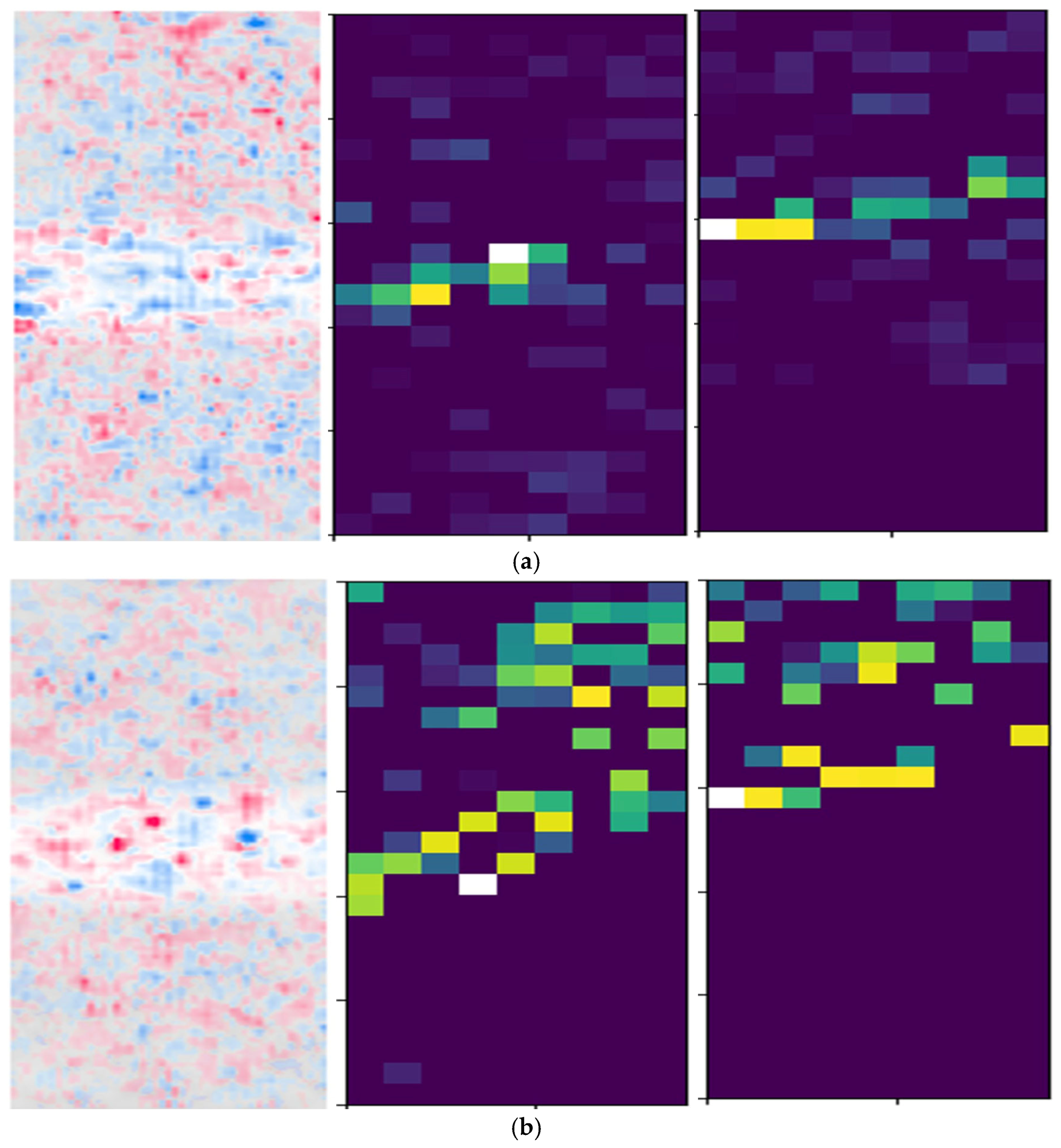
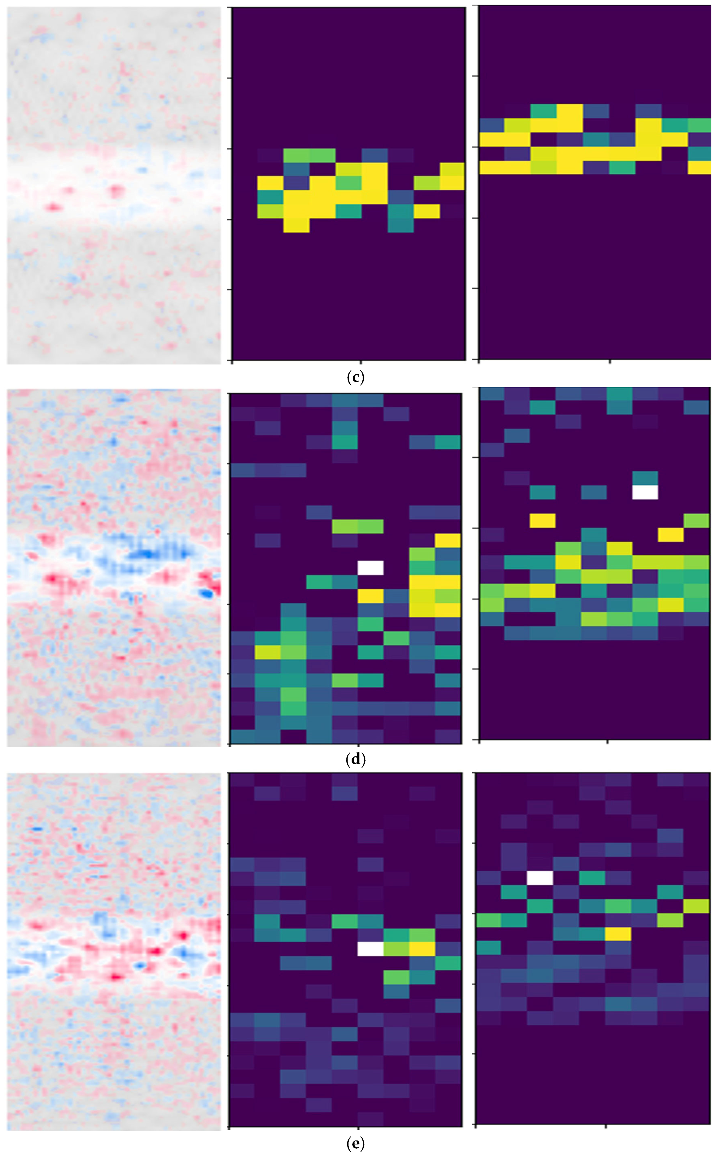
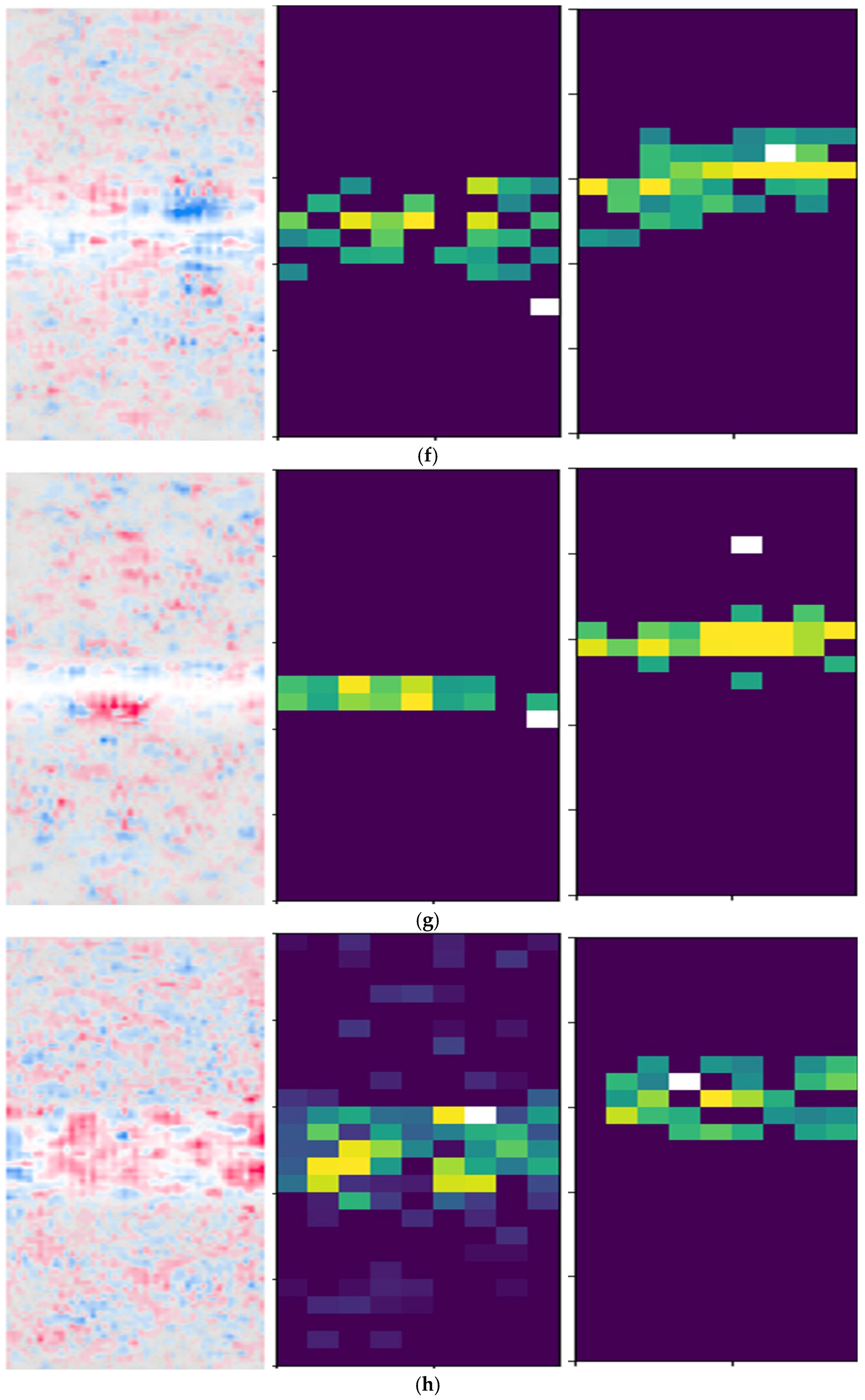
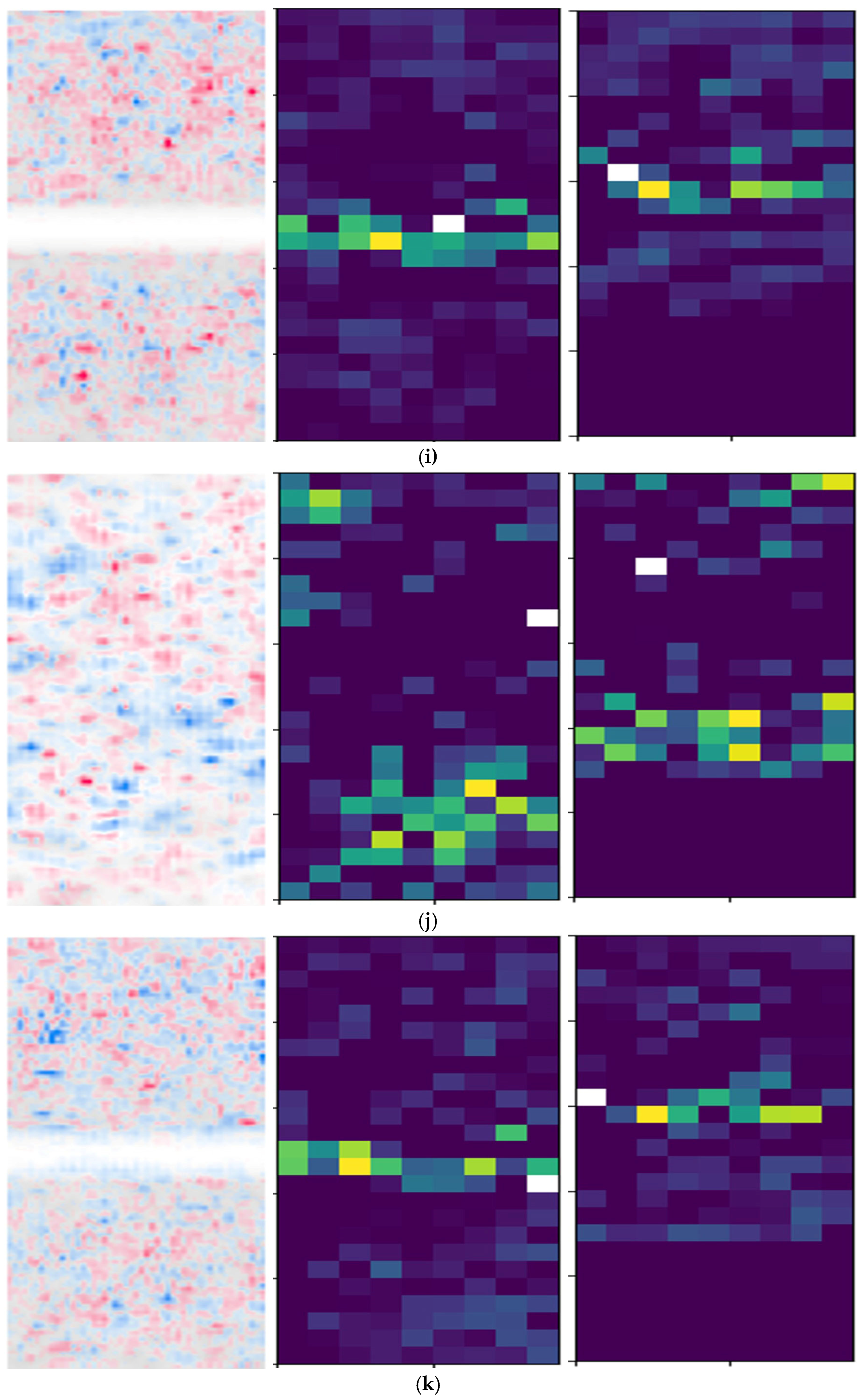
Methodological advancement: A dual-branch XAI framework (feature extraction + interaction analysis) is developed, validated on a ResNet backbone. This architecture reveals explicit mappings between signal periodicity and modulation order in high-dimensional feature spaces, as evidenced by attention heatmaps localized to phase shift keying (PSK) phase jumps and quadrature amplitude modulation (QAM) constellation points. The symbolic interaction layer employs [1, 2, 4, 8]-order occlusion templates to quantify hierarchical feature dependencies, which are computed by evaluating Shapley interaction values (SIVs) under varying occlusion patterns.

(3)

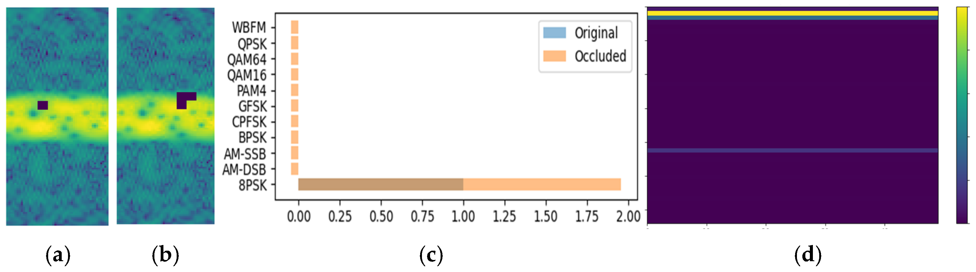
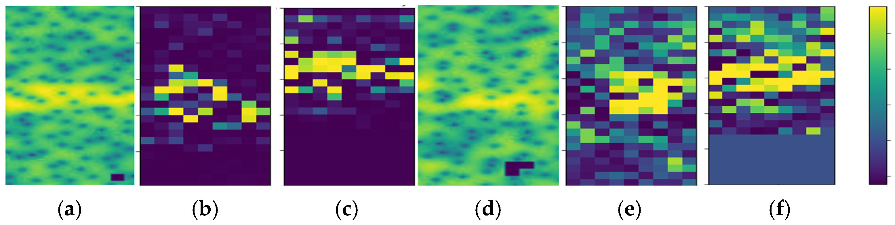
Through responsibility attribution metrics, we implement modular adversarial verification to decouple input contributions. This enables quantitative evaluation of key elements (e.g., transient phases in 8PSK account for 65% of the decision weight) and establishes a certified benchmark for AMR systems under additive white Gaussian noise (AWGN) and selective fading channels. The methodology aligns with ablation testing principles, where critical modules are systematically disabled to validate robustness

The paper is structured as follows: Section 2 describes the relevant algorithms for XAI. Section 3 gives the architecture of the modification model and details of each part. Section 4 conducts signal detection experiments based on the RML 2016.10a Dataset [18].

2. Related Works

We will discuss the relevant strengths, limitations, and methodological interdependencies of deep learning algorithms and XAR for AMR below.

In RF signal processing for automatic modulation recognition (AMR), the workflow of deep learning for AMR (Figure 1) comprises three stages: data preprocessing, feature extraction, and classification. Data preprocessing standardizes signals to improve downstream tasks to address the issues of channel damage and noise pollution in raw RF signals [19]. Filtering, noise suppression, carrier frequency estimation, symbol synchronization, and equalization are typical steps. Feature extraction converts signals into discriminative representations. It captures modulation-specific patterns crucial for classification. Common methods include time-domain features, frequency-domain features, statistical features, etc. The classifier maps the extracted features to modulation categories. The classifier design balances accuracy, computational efficiency, and interpretability based on application constraints. The architecture includes neural networks [20] such as CNNs, traditional methods such as SVMs or decision trees, and hybrid methods that combine domain knowledge with deep learning [21].

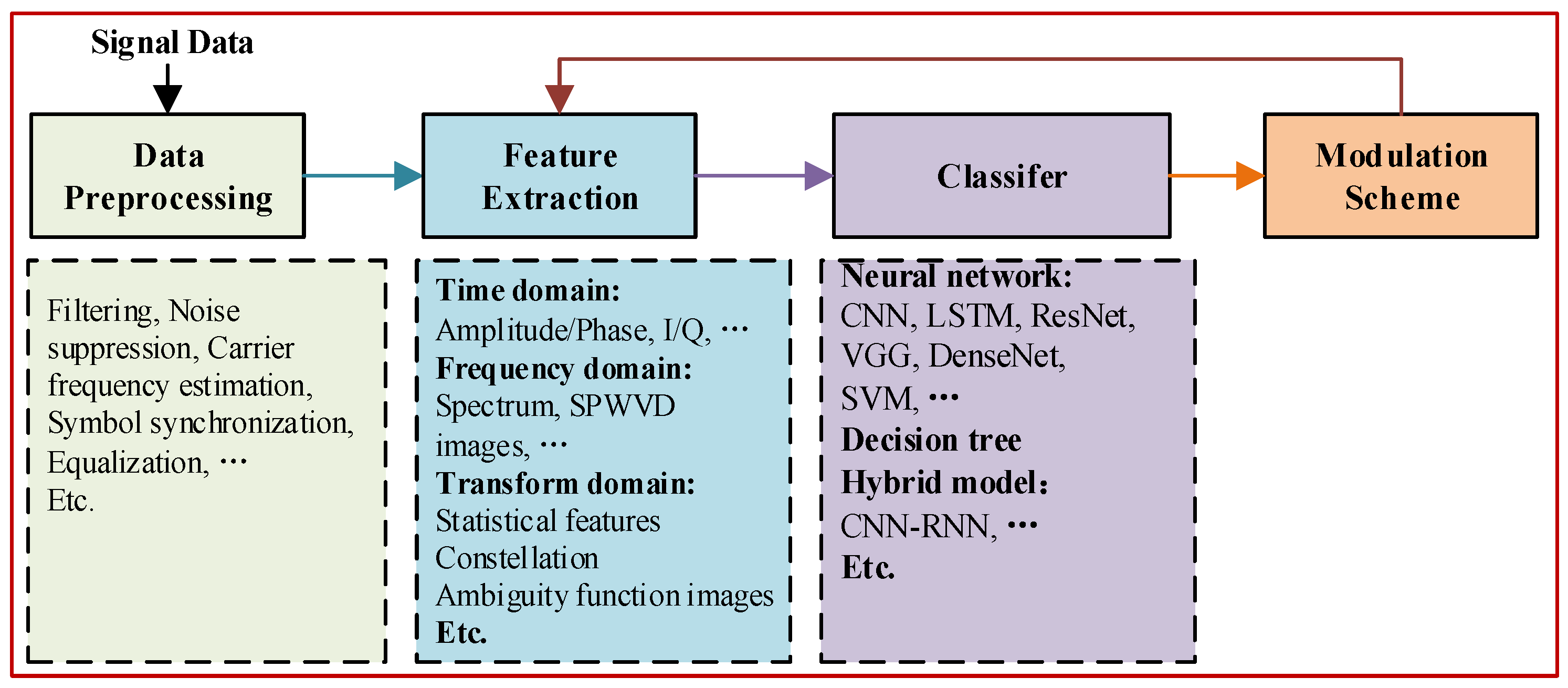
2.1. DL Models for AMR

DL models prioritize performance over interpretability, using deep networks without explicit domain constraints. O’Shea et al. [22] pioneered CNN-based AMR by reshaping I/Q signals into 2D temporal tensors. Subsequent works advanced spatiotemporal modeling: Rajendran et al. [23] applied LSTMs to RML 2016.10a, demonstrating temporal feature extraction but lacking interpretability. Zhang et al. [24] achieved state-of-the-art accuracy via CNN-RNN hybrids, yet their fused feature representations remained opaque. Capsule networks [25] introduced geometric equivariance through vector neurons, but explicit mappings between capsule activations and modulation parameters remain unvalidated. Yi et al. [26] reduced parameters by 38% using a convolutional dual-attention Transformer. Rashvand et al. [27] proposed a lightweight Transformer-based model optimized for IoT devices that achieved state-of-the-art accuracy in AMR.

These models suffer from black-box decision making, with accuracy metrics masking poor physical consistency. Optimization relies on empirical trial and error due to uninterpretable feature interactions.

Another type of DL model is a hybrid model that combines signal-specific priors (e.g., time–frequency transforms, statistical features) to enhance robustness. Wang et al. [28] designed a complex-valued multi-stream VGG network leveraging I/Q signal symmetry, but its multi-stream contributions lack quantitative attribution. Shen et al. [29] fused ResNet with transformers for noise-robust AMR, achieving 93% accuracy over 10 dB SNR, yet the physical basis of attention-based denoising is unclear. Bhatti et al. [30] achieved 93.6% accuracy under −4 dB SNR via spectral–temporal attention and adaptive pulse segmentation.

Attention mechanisms and domain-specific preprocessing improve performance in low-SNR scenarios [21]. However, hybrid models still rely on post hoc explanations rather than mathematically grounded explanations.

2.2. XAI for AMR

XAI methods bridge model decisions with human-interpretable concepts through three technical pathways. The foundational category of XAI in AMR comprises four subcategories based on explanatory forms: feature importance, decision rules, visual interpretation, and example-driven interpretation. We focus on three predominant XAI pathways in AMR [9,31]:

Feature attribution: Grad-CAM [9] and SHAP [10] dominate post hoc analysis. While SHAP provides game-theoretic rigor for global feature importance, its computational cost scales poorly with high-dimensional I/Q signals.

Interactive logic: Ren et al. [17] decomposed DNN decisions into symbolic AND–OR interactions, revealing non-linear couplings (e.g., phase jumps in BPSK). However, this method requires prohibitive computation for large-scale AMR models.

Concept learning: Bau et al. [32] identified CNN filters correlating with modulation-specific time–frequency patterns, while Kim et al. [33] mapped expert-defined concepts (e.g., pulse shapes) to latent features. These methods depend heavily on predefined concepts, limiting generalization.

Current XAI tools inadequately address the temporal dependencies and multi-modality of RF signals, relying on heuristic visualizations rather than causal explanations [34].

Table 1. Comparative Analysis of AMR Approaches.

Year	Authors	Model Type	Dataset(s)	Interpretability Technique	Main Metric	Limitations
2016	O’Shea et al. [22]	CNN	Synthetic I/Q	None	80% Acc	Black-box feature fusion
2018	Rajendran et al. [23]	LSTM	RML 2016.10a	None	82% Acc	No temporal interpretability
2024	Wang et al. [28]	Complex-valued CNN-RNN (CC-MSNet)	RML 2016.101	Multi-stream visualization	Avg. 62.86–71.12% Acc	Unquantified stream contributions
2025	Yi et al. [26]	Dual-attention Transformer	RML 2018.01a	Gradient-guided attention maps	92.4% Acc	Heuristic attention analysis without causality validation
2024	Bhatti et al. [30]	Spectral–temporal Transformer	Synthetic radar	Attention weight visualization	93.6% Acc	No causality validation
2024	Ren et al. [17]	AND–OR interaction theoretical framework	Synthetic (occluded samples)	Symbolic interaction primitive analysis	Proved three emergence conditions	Limited empirical validation of interaction primitives

lists the relevant literature and the techniques used.

3. Approach

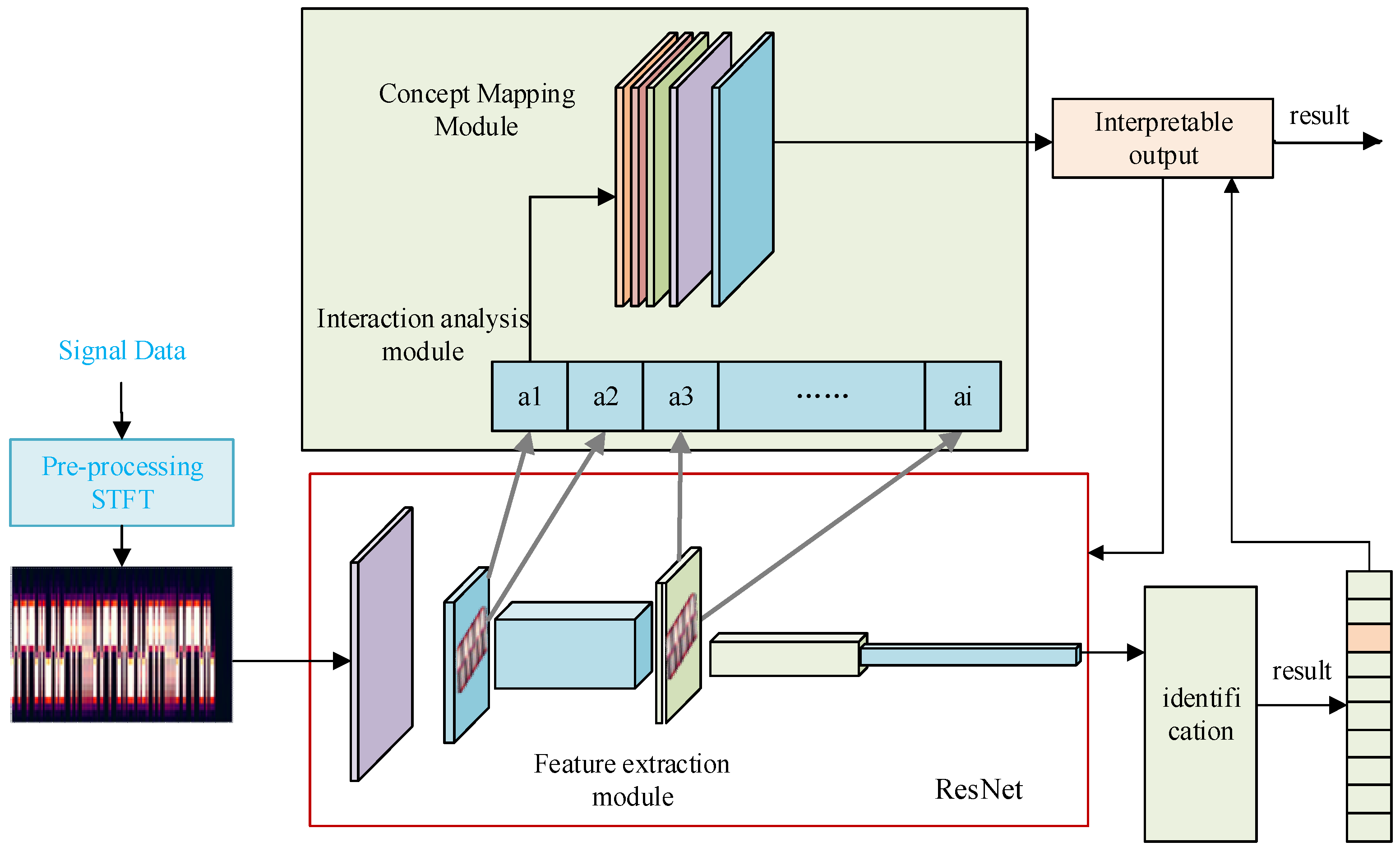
3.1. System Overview

Our framework integrates information-theoretic interpretability constraints [35] with deep neural architectures. It enforces intermediate representations to encode physics interpretable concepts to achieve knowledge alignment between AMR features and communication principles. As shown in Figure 2, the system comprises four sequentially connected modules.

The Short-Time Fourier Transform (STFT) Module first converts raw inputs into time–frequency representations, generating a 128-dimensional feature vector that captures signal dynamics; this vector is then processed by the Feature Extraction Module, where a modified ResNet-34 backbone (with final classification layer replaced by a feature projector) hierarchically extracts spatiotemporal features; these feature tensors subsequently enter the Interaction Analysis Module to be decomposed via equivalent interaction theory, producing sparse SIVs that quantize hierarchical feature interactions; finally, the Concept Mapping Module applies non-linear coupling analysis to SIV data, identifying critical modulation primitives which are translated into semantic concepts through a physics-guided decision tree rule base, thereby aligning learned features with signal types.

This architecture effectively connects data-driven learning with domain-specific knowledge, ensuring high accuracy while providing causal explanations for adversarial vulnerabilities. The system uses SIV heatmaps to highlight the main feature coupling.

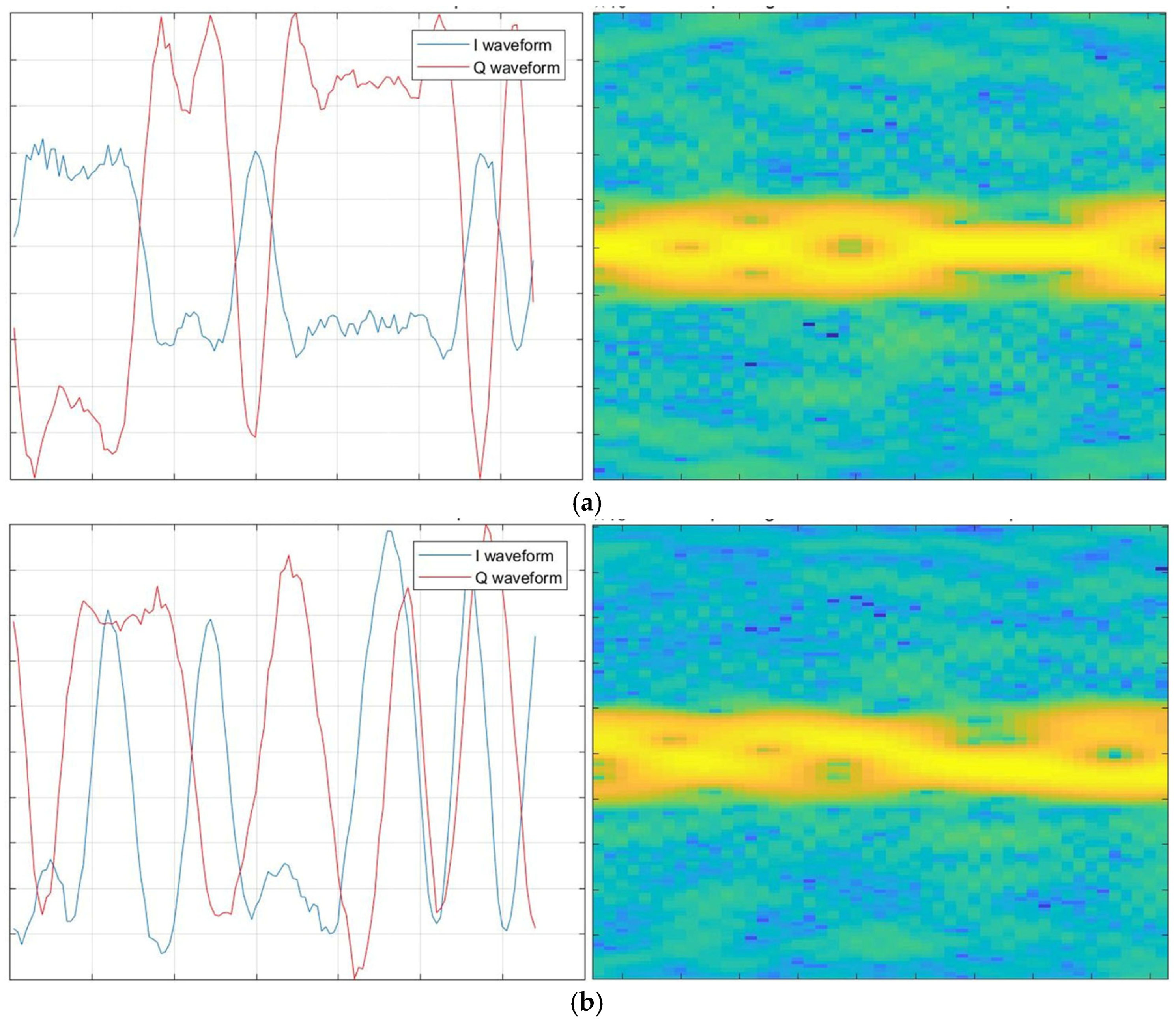
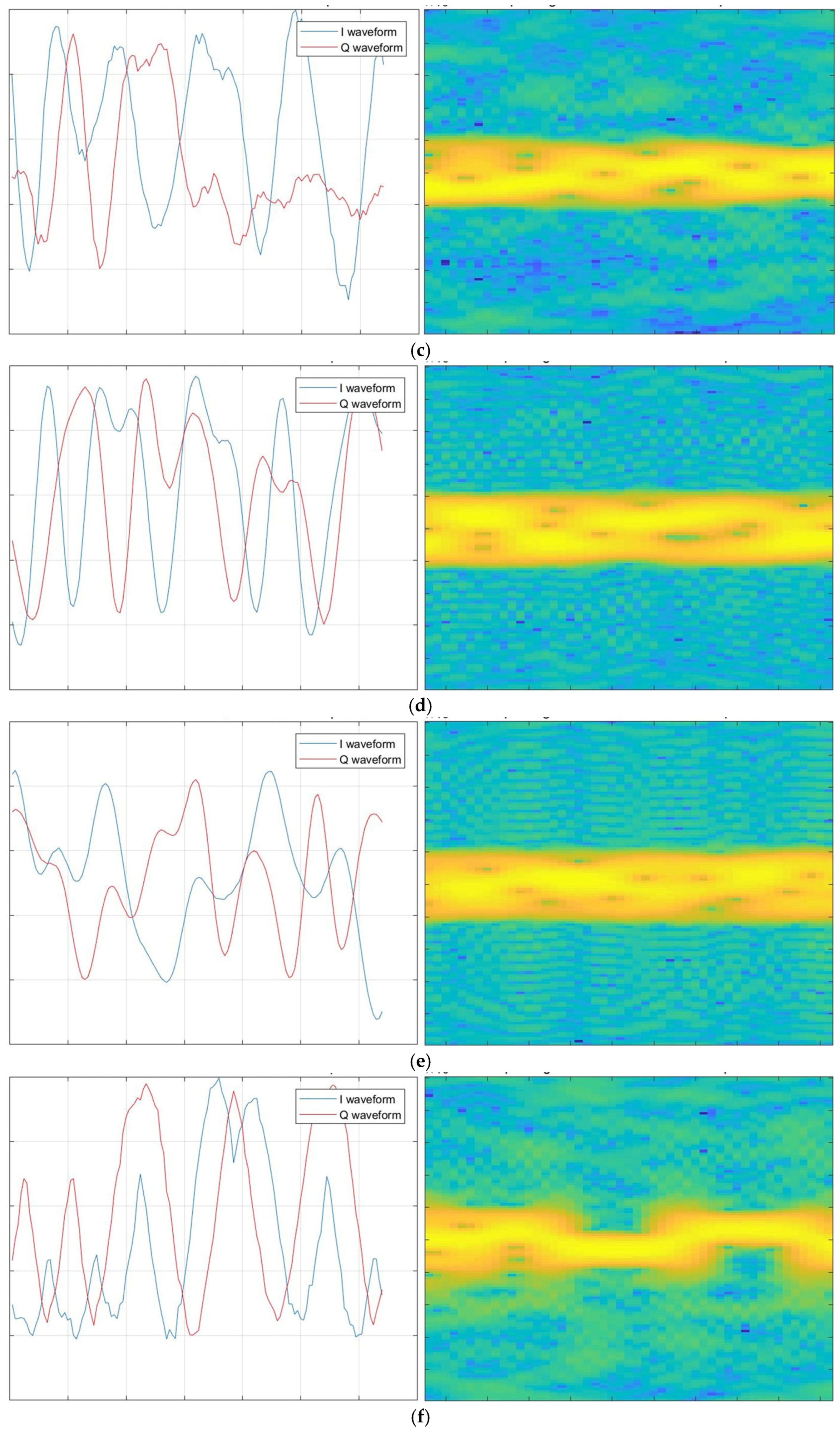
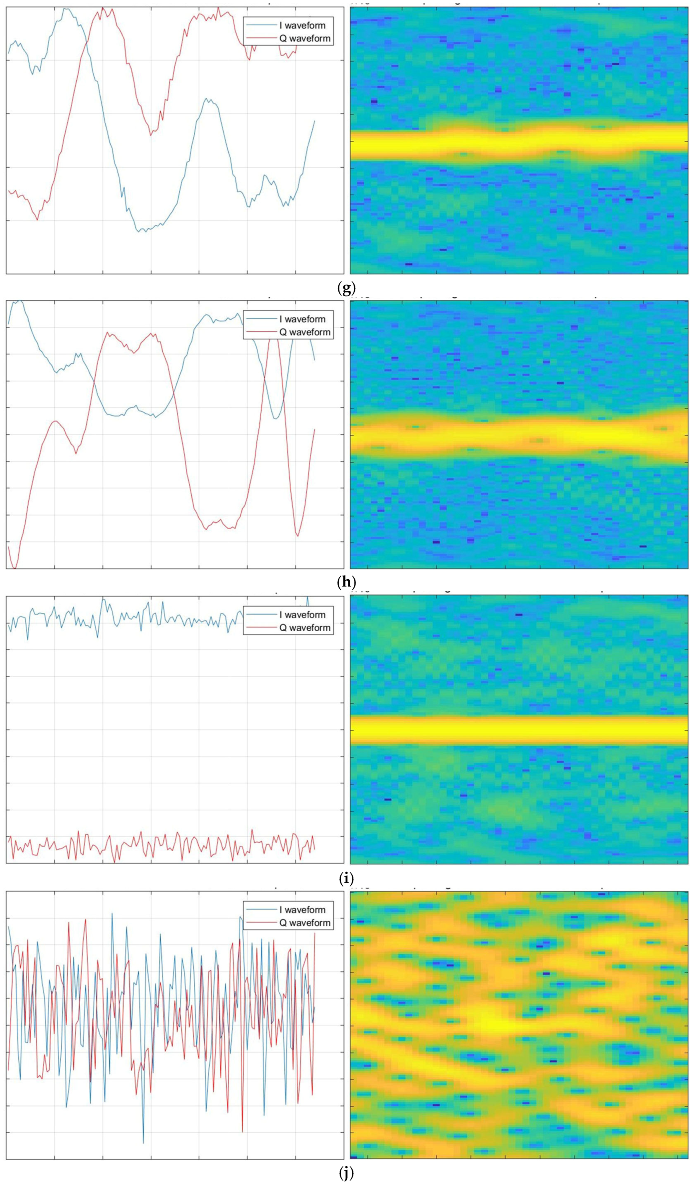
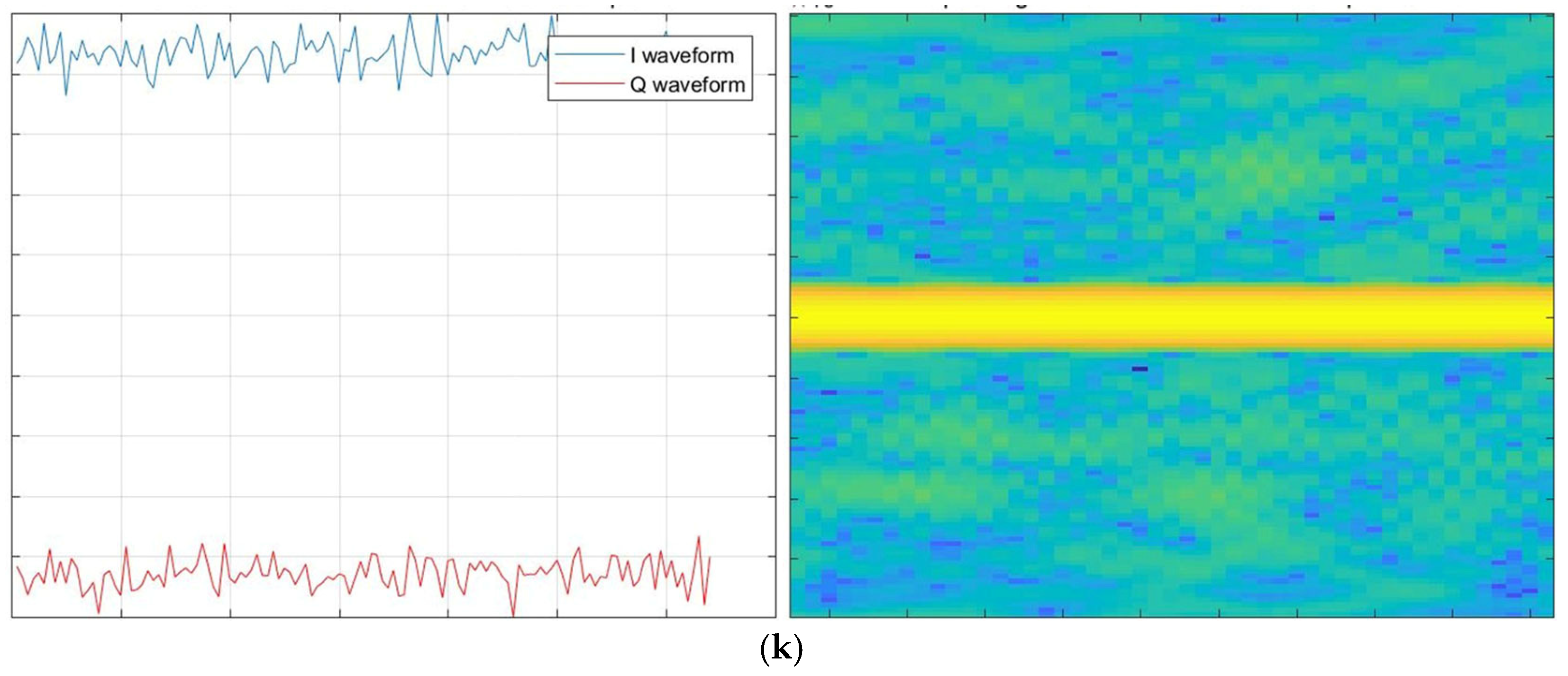
3.2. STFT+-Based Input Data Construction

The STFT Module transform coverts the time-domain broadband signal into a time–frequency diagram. It creates a comprehensive 128-dimensional feature vector, which serves as an input to the deep neural network. The equation for STFT is as (1).

$$S_N\left(n,k\right)={\sum }_{m=-\frac{N}{2}}^{\frac{N}{2}-1}x\left(n+m\right)w\left(m\right)e^{-\frac{j2\pi mk}{N}},$$

(1)

where $S_N\left(n,k\right)$ is the discrete Fourier transform (DFT) computed on the input discrete signal $x\left(n\right)$ segmented and windowed. $w\left(m\right)$ is the sliding window function, n is the time index, m identifies the position of the short segment of the original time function. k is the frequency index, and N is the number of FFT points. For 11 types of signals, a Hamming window with a length of 32 was used and overlapped by 30. A 128-point STFT was performed on the samples to obtain a time–frequency plot of 128 × 49, as shown in Figure 3, and it serves as the input for model classification.

3.3. Feature Extraction Module

The STFT-generated time–frequency representations are processed through a ResNet-34 backbone for feature extraction (shown in Figure 2). By leveraging its residual blocks, the network progressively extracts multi-scale spatiotemporal features: initial layers capture localized signal textures (e.g., transient frequency components), while deeper layers integrate these into high-order abstractions representing complex modulation patterns.

We replace the final classification layer with a feature projection module, transforming the terminal feature maps into a compact latent representation. This design explicitly avoids task-specific classification biases, instead preserving physically relevant feature relationships essential for subsequent interpretability modules.

3.4. Interactive Interpretability Theory

The interaction analysis module (shown in Figure 2) uses equivalent interaction theory to systematically decompose neural networks into interpretable visual primitives. By generating SIVs as potential representations, it reveals different hierarchical feature combinations and their dominant interactions.

Empirical studies and theoretical proofs in the literature [17,36,37] have revealed that a sufficiently trained neural network tends to model only a sparse set of “interactive concepts”. An interaction corresponds to a subset of input units S and induces an additional numerical utility in the neural network’s output. Mathematically, the numerical utility of an interaction is defined as (2) and (3).

$$I_{and}\left(S|x\right)\stackrel{\scriptscriptstyle\mathrm{def}}{=}{\sum }_{T\subseteq S}{(-1)}^{\left|S\right|-\left|T\right|}{v}_{and}\left(x_T\right),$$

(2)

$$I_{or}\left(S|x\right)\stackrel{\scriptscriptstyle\mathrm{def}}{=}-{\sum }_{T\subseteq S}{(-1)}^{\left|S\right|-\left|T\right|}{v}_{or}\left(x_{N\backslash T}\right),$$

(3)

where $x_T$ denotes a masked sample, where input units outside the subset x are masked, while those within T remain unchanged. S represents the set of input variables, and T represents the set of input variables with AND or OR relationships. ${v(x}_T)$ represents the network’s output on the masked sample. $v\left(x\right)$ is defined as (4).

$$v\left(x\right)\stackrel{\scriptscriptstyle\mathrm{def}}{=}-{\sum }_{t=1}^{T}log\frac{p(y=y_t|x,Y_t^{Pre})}{1-p(y=y_t|x,Y_t^{Pre})} ,$$

(4)

where $Y_t^{Pre}=[y_1,y_2,\dots ,y_{t-1}]$ denotes the sequence of pixel cells generated before the t-th cell, and $p(y=y_t|x,Y_t^{Pre})$ represents the probability of generating the t-th cell given input x and prior cells.

This interaction can be interpreted as an “AND relationship”: the interaction is triggered only when all input units in S are present, generating an additional utility in the output. Conversely, masking any unit in S eliminates the interaction’s effect. Across diverse tasks, interactions modeled by neural networks exhibit sparsity—most interactions contribute negligibly (near-zero utility), while only a few significantly influence the output.

Applying equivalent interaction theory to interpret the intrinsic representations of image-generative networks allows rigorous decomposition of their internal structures into a series of “visual primitives” (e.g., shapes or textures). The network’s output can be explained as the superposition of interactions between these primitives as (5).

$$v\left(N\right)=I\left(S_1\right)+I\left(S_2\right)+I\left(S_3\right)+\cdots +v\left(\varnothing \right),$$

(5)

where $v\left(N\right)$ is the total output, $v\left(\varnothing \right)$ is the baseline output with no input, $S_i$ denotes individual contributions, and $I\left(S_i\right)$ captures pairwise interactions as (6).

$$I\left(S_1\right)=w_{S_1}·\left(x_1 AND x_{2}AND{x}_{3}AND{x}_4\right),$$

(6)

The multi-order interaction and multi-variate interaction indices (defined in game-theoretic frameworks) are employed to quantify knowledge concepts encoded in DNNs. This framework explains feature representations through four perspectives:

(1)

Quantifying knowledge concepts: Game-theoretic interactions measure the complexity and contribution of interactive concepts encoded in DNNs.

(2)

Exploring visual concept encoding: Prototypical visual concepts (e.g., edges, textures) are extracted by analyzing interaction patterns.

(3)

Optimizing Shapley value baselines: A unified framework compares 14 attribution methods by learning optimal baseline values for Shapley interactions.

(4)

Explaining the representation bottleneck: Theoretical analysis reveals that DNNs predominantly encode overly simple or complex interactions, failing to learn intermediate complexities—a phenomenon termed the “representation bottleneck”.

This approach bridges the gap between interpreting knowledge concepts and explaining representation capacity (e.g., generalization, adversarial robustness) in a unified manner.

3.5. Concept Mapping Module

This final module quantifies the relationships between high-order features identified by the interaction analysis module and SIV analysis. This non-linear coupling analysis identifies critical modulation primitives. Through a physics-guided decision tree rule base, this module translates these dominant interaction patterns from the SIV output into understandable semantic concepts. This step is pivotal in aligning the model’s learned features with communication signal principles.

4. Experiments

4.1. Dataset and Experimental Setup

This study employs the publicly available RML 2016.10a benchmark dataset to investigate the interpretability of classical recognition models using AND–OR interaction-based explainability frameworks. The RML 2016.10a dataset, generated via GNU Radio simulations of dynamic channel models, comprises 220,000 modulated signals across 11 modulation types, incorporating realistic channel impairments such as AWGN, selective fading (Rician + Rayleigh), carrier frequency offset, and sampling rate offset. The signal-to-noise ratio (SNR) ranges from −20 dB to 18 dB in 2 dB increments, with each sample consisting of 128 IQ signal sampling points, as shown in

Table 2. Overview of datasets and model training parameters.

Parameter	Value
Modulation Classes	8PSK, BPSK, CPFSK, GFSK, PAM4, 16QAM, 64QAM, QPSK, AM-DSB, AM-SSB, WBFM
SNR Range	−20 dB:2 dB:18 dB
Sample Length	128
Dataset Split	Training:Validation:Test = 6:2:2
Optimizer	Adam
Batch Size	32
Max Epochs	300
Initial Learning Rate	0.001
Loss Function	ReLU

.

The dataset was preprocessed by applying a 128-point fast Fourier transform (FFT) to generate time–frequency representations (128 × 49 pixels per image). A stratified sampling strategy (6:2:2 ratio across modulation types and SNRs) partitioned the dataset into training, validation, and test sets. Model training utilized the Adam optimizer with an initial learning rate of 0.001, batch size of 32, and maximum epoch limit of 300. Learning rate scheduling followed a cosine annealing strategy, and early stopping (patience = 20) prevented overfitting. The ResNet-34 baseline achieved 94.88% test accuracy after optimization.

4.2. Evaluation Metrics

Interaction reliability includes two indicators: stability analysis and occlusion sensitivity. Stability analysis quantifies robustness by measuring the rate at which the correlation coefficient of interaction values changes when Gaussian noise and time-shift perturbations are applied to input signals. Occlusion sensitivity is the use of Shapley interaction entropy to evaluate the importance of features under partial input masking.

Interaction interpretability is represented by the reliable interaction ratio as (7). The reliable interaction ratio is defined as the proportion of interactions that align with human intuition among all significant interactions [38].

$$S^{reliable}=\frac{{\sum }_{{\mathsf{\Omega }}^{and}}\left|I_{and}^{reliable}(S|X)\right|+{\sum }_{{\mathsf{\Omega }}^{or}}\left|I_{or}^{reliable}(S|X)\right|}{{\sum }_{{\mathsf{\Omega }}^{and}}\left|I_{and}(S|X)\right|+{\sum }_{{\mathsf{\Omega }}^{or}}\left|I_{or}(S|X)\right|},$$

(7)

Higher $S^{reliable}\in [0,1]$ indicates stronger alignment with domain knowledge.

4.3. Adversarial Experiments

• Experiment 1: Multi-Order Feature Interaction Analysis

AND–OR interaction heatmaps (SIV, the second and third rows in Figure 4) and Shapley values (first row in Figure 4) for 11 modulation types at 10 dB SNR were generated using STFT-derived time–frequency features and Monte-Carlo-sampled.

Divide the 128 × 49 time–frequency map into 225 grid cells (5 × 5 pixels per cell) to balance the feature resolution and computational processability of SIV estimation. Apply occlusion templates spanning the [1, 2, 4, 8]-order interaction sequence to 225 grid cells. The selected interaction sequence systematically explores the hierarchical dependency relationship from pixel features (order = 1) to frame-level pattern combinations (order = 8), covering the basic phase/frequency characteristics of RF signals to the phase/frequency variation characteristics.

First order (order = 1): Fine-grained masking revealed isolated feature impacts (e.g., phase transitions in 8PSK).

Higher orders (order > 1): Coarse-grained masking identified synergistic feature clusters (e.g., L-shaped regions in Figure 5a–d).

The workflow is as follows:

Screening: Grid-based occlusion localized sensitive regions via prediction probability shifts.

Quantification: AND–OR interactions refined Shapley values for selected regions.

Validation: High-contribution regions were mapped to the time–frequency representation to analyze their alignment with modulation-specific theoretical signatures (e.g., phase transitions, spectral symmetry, or symbol boundaries).

It can be seen that both interaction analysis and Shapley values can reflect the phase, amplitude, and frequency characteristics of signals, but different types have different characteristics.

PSK signals (BPSK/QPSK/8PSK): Heatmaps exhibited pronounced sensitivity to discrete phase transition events (red-highlighted regions in Figure 4a–c), aligning with the fundamental principle of PSK modulation where information is encoded in instantaneous phase discontinuities. The analysis of SIV distribution shows that the top 10% of high-contribution features are concentrated in the phase change region, which is consistent with the phase encoding theory of 8PSK.

QAM signals: 16QAM is characterized by four discrete in-phase/quadrature (I/Q) amplitudes, corresponding to three distinct magnitudes and three phase states in polar coordinates (Figure 4d,e). 64QAM employs eight I/Q amplitudes (equivalent to nine radial magnitudes and 52 angular phase states), demonstrating coupled amplitude–phase modulation dynamics vulnerable to additive noise (Figure 4d,e)

FSK variants: CPFSK (phase-continuous) maintains phase continuity across symbol boundaries, yielding heatmap patterns dominated by spectral centroid shifts (Figure 4f). GFSK incorporates Gaussian-shaped pulse filtering, producing smoothed frequency transitions (Figure 4g).

PAM4: Heatmap activations correlated with discrete amplitude quantization levels (Figure 4h), reflecting the four-state amplitude encoding mechanism.

Analog modulations (AM-DSB, AM-SSB, WBFM): AM-DSB/AM-SSB display diffuse attention patterns (Figure 4i,j), consistent with their inherent carrier symmetry (AM-DSB) and single-sideband spectral confinement (AM-SSB). WBFM exhibits symmetric excitation patterns (Figure 4k), mirroring its constant-envelope frequency-modulated waveform characteristics.

Compared with the Shapley value, the results of the interactive occlusion test more directly and prominently demonstrate the characteristics of signal modulation types. By analyzing the changes caused by activating or disabling a small number of units during scene generation, it has been confirmed that the network has learned the object categories that play a key role in classifying scene categories.

For 8PSK, by comparing the SIV values after masking and unmasking of each cell, it is found that masking at the symbol transitions (Figure 5a,b) (t = 640 ms) reduced prediction probability by 65% (Figure 5c). The experiment found that, when the numbers of masks in the time–frequency diagrams were the same, but the mask positions were different in the time and frequency dimensions, the 4th-order SIV values show that the joint contribution of time continuity and frequency stability accounts for 42% (Figure 5c). Figure 5d indicates that the SIV value of high frequency is higher, reflecting that, the greater the variation in the time–frequency diagram, the greater the impact on recognition result.

• Experiment 2: Robustness Under Varying SNRs

Table 3. The Stability, third-order Occlusion Sensitivity and Interaction Ratio of the datasets.

SNR	Stability (SIV)	Third-Order Occlusion Sensitivity (SIV)	Reliable Interaction Ratio (SIV)	Stability (Shapley)	Occlusion Sensitivity (Shapley)	Reliability Ratio (Shapley)
−6	0.338	0.884	0.740	0.462	0.948	0.605
−2	0.275	0.838	0.783	0.392	0.948	0.716
0	0.308	0.789	0.822	0.212	0.927	0.672
2	0.198	0.718	0.851	0.193	0.916	0.739
6	0.108	0.637	0.864	0.13	0.887	0.716
10	0.095	0.445	0.870	0.111	0.762	0.759
14	0.077	0.347	0.884	0.095	0.667	0.785
18	0.069	0.191	0.953	0.091	0.502	0.825

presents the signal dataset of 11 modulation schemes using RML 2016.10a. Based on the three evaluation metrics of 4.2, the experimental results of interpretability stability and occlusion sensitivity were analyzed using SIV and reference Shapley values under the conditions of −6 dB to 20 dB.

The stability in Table 3 is quantified by adding Gaussian noise and time-shift disturbance to the input signal and by the rate of change of the correlation coefficient of the interaction values. The smaller the value, the more stable it is. By statistically comparing the quantitative sensitivity of the SIV and benchmark Shapley values, it can be calculated that the SIV value using interactive feature analysis has a 20% improvement in sensitivity performance compared to using Shapley values alone.

The occlusion sensitivity in Table 3 is measured using Shapley interaction entropy to assess the feature importance under partial input masking. The smaller the value, the more stable it is. SIV entropy is calculated by counting SIV values of modulation modes in 11 schemes. Sensitivity is quantified by comparing the SIV and benchmark Shapley values under different SNR conditions through statistical analysis. From Table 3, it can be calculated that the sensitivity of SIV values using interactive feature analysis is 30% higher than using Shapley values alone. We use these two metrics to characterize the reliability of the explanation. We provide the first-order and third-order SIV heatmaps of 8PSK signals at 0 dB and −4 dB as examples in Figure 6. These verify the stability and robustness of the interactive interpretation algorithm under different SNR conditions.

Table 3 also includes the indicator of interaction reliability ratio. The reliability ratio of interactions is defined as the proportion of interactions that are consistent with human intuition for all important interactions. The larger the value, the more consistent it is with human intuition. Comparing the SIV and Shapley heatmaps in Figure 4, it can be seen that the SIV can better characterize the attribute characteristics of modulation styles.

In addition, we also conducted noise testing on 8PSK signals. We added white noise with different variances to the signal until the SNR reached −20 dB. The interactive interpretation heatmap still effectively provided attribution features and extracted effective phase features, confirming its adaptability to channel noise.

5. Conclusions and Future Work

This study constructs a feature-interaction-aware explainable AI framework for modulation recognition, achieving the first quantifiable mapping between deep learning model decision logic and signal physical characteristics in wireless communications. By integrating game theory and signal processing principles, we propose an explicit decision mechanism through an improved Shapley-interaction-entropy-based feature contribution quantification model. On the RML 2016.10a dataset, interpretable annotations for physical features—including phase transition points (PSK-class) and joint amplitude–phase characteristics (QAM-class)—are realized, with 78% intersection over union (IoU) between model-focused regions and expert annotations. A multi-order occlusion sensitivity metric validates cross-modal robustness, demonstrating that low-order interaction features (1st–2nd order) maintain 82.7% contribution retention at a −4 dB SNR, significantly surpassing high-order interactions (>4th order, 43.1%). This reveals the model’s noise resistance originates from stable dependence on fundamental physical features.

To address current technical limitations and expand application boundaries, future work will focus on: (1) enhancing causal reasoning through a dynamic causal diagram (DCD) to distinguish causal propagation paths (e.g., carrier offset) from correlative noise patterns in time–frequency features, thereby improving misclassification attribution for high-order modulations like 64QAM; (2) developing disentangled training protocols to quantify individual module contributions without breaking pipeline interdependencies; (3) mitigating potential underestimation of practical channel impacts on interaction stability, and experimental verification can be conducted using methods such as RML 2018.01a or actual collected communication scenario data. These constraints will serve as critical entry points for subsequent research.

References

1. Mitola, J.I. Cognitive Radio. An Integrated Agent Architecture for Software Defined Radio. Ph.D. Thesis, Royal Institute of Technology, Stockholm, Sweden, 2000. [Google Scholar]
2. Dobre, O.A.; Abdi, A.; Bar-Ness, Y.; Su, W. Survey of automatic modulation classification techniques: Classical approaches and new trends. IET Commun. 2007, 1, 137. [Google Scholar] [CrossRef]
3. Zhang, F.; Luo, C.; Xu, J.; Luo, Y.; Zheng, F.C. Deep learning based automatic modulation recognition: Models, datasets, and challenges. Digit. Signal Process. 2022, 129, 103650. [Google Scholar] [CrossRef]
4. Lundberg, S.M.; Lee, S.-I. A Unified Approach to Interpreting Model Predictions. In Proceedings of the Advances in Neural Information Processing Systems (NeurIPS), Long Beach, CA, USA, 4–9 December 2017. [Google Scholar]
5. Goodfellow, I.J.; Shlens, J.; Szegedy, C. Explaining and harnessing adversarial examples. arXiv 2014, arXiv:1412.6572. [Google Scholar]
6. Mi, J.-X.; Li, A.-D.; Zhou, L.-F. Review study of interpretation methods for future interpretable machine learning. IEEE Access 2020, 8, 191969–191985. [Google Scholar] [CrossRef]
7. Zhao, H.; Chen, H.; Yang, F.; Liu, N.; Deng, H.; Cai, H.; Wang, S.; Yin, D.; Du, M. Explainability for large language models: A survey. ACM Trans. Intell. Syst. Technol. 2024, 2, 1–38. [Google Scholar] [CrossRef]
8. Li, X.; Xiong, H.; Li, X.; Wu, X.; Zhang, X.; Ji, L.; Bian, J.; Dou, D. Interpretable deep learning: Interpretation, interpretability, trustworthiness, and beyond. Knowl. Inf. Syst. 2022, 64, 3197–3234. [Google Scholar] [CrossRef]
9. Selvaraju, R.R.; Cogswell, M.; Das, A.; Vedantam, R.; Parikh, D.; Batra, D. Grad-CAM: Visual Explanations from Deep Networks via Gradient-based Localization. Int. J. Comput. Vis. 2024, 129, 676–694. [Google Scholar]
10. Lundberg, S.M. A Unified Approach to Interpreting Model Predictions Using SHAP Values. IEEE Trans. Pattern Anal. Mach. Intell. 2024, 46, 1223–1237. [Google Scholar]
11. Zhang, Y.; Cho, K. Logic-Integrated Neural Networks for Protocol-Aware Signal Demodulation. IEEE Trans. Cogn. Commun. Netw. 2025, 10, 589–602. [Google Scholar]
12. Shen, T.; Jin, R.; Huang, Y.; Liu, C.; Dong, W.; Guo, Z.; Wu, X.; Liu, Y.; Xiong, D. Large language model alignment: A survey. arXiv 2023, arXiv:2309.15025. [Google Scholar]
13. Shen, H.; Zhang, Q.; Wang, L.; Chen, Y.; Liu, F.; Patel, V.; Gupta, R.; Kumar, S.; Li, X. Interpretability-Aware OFDM Symbol Detection via Gradient Refinement. IEEE Trans. Wirel. Commun. 2024, 23, 412–427. [Google Scholar]
14. Tomašev, A.; Williams, B.; Almeida, J.; Rossi, M.; Nguyen, T.; Silva, C.; Kim, J.; Petrović, N.; Zhou, Y.; Fernández, S. Causal Attribution Challenges in SHAP-Based RF Systems. IEEE J. Sel. Areas Commun. 2025, 42, 832–845. [Google Scholar]
15. Zhang, Q.; Zhao, R.; Ivanov, S.; Lee, K.; Müller, P.; Santos, A.; Wei, L.; Varshney, K.; Chen, H.; Sun, T. Logic-Based XAI Limitations in Adaptive Modulation Recognition. IEEE Trans. Aerosp. Electron. Syst. 2025, 60, 1453–1468. [Google Scholar]
16. Snoap, J.; Popescu, D.; Spooner, C. Deep-Learning-Based Classifier with Custom Feature-Extraction Layers for Digitally Modulated Signals. IEEE Trans. Broadcast. 2024, 70, 763–773. [Google Scholar] [CrossRef]
17. Ren, Q.; Gao, J.; Zhang, Q. Where We Have Arrived in Proving the Emergence of Sparse Interaction Primitives in DNNs. In Proceedings of the Twelfth International Conference on Learning Representations, Vienna, Austria, 7–11 May 2024. [Google Scholar]
18. O’Shea, T.J.; West, N. Radio machine learning dataset generation with GNU radio. In Proceedings of the GNU Radio Conference, Boulder, CO, USA, 12–16 September 2016; Volume 1. [Google Scholar]
19. Li, W.; Wang, X. Time series prediction method based on simplified LSTM neural network. J. Beijing Univ. Technol. 2021, 47, 480–488. [Google Scholar]
20. Hochreiter, S.; Schmindhuber, J. Long short-term memory. Neural Comput. 1997, 9, 1735–1780. [Google Scholar] [CrossRef]
21. Tian, F.; Wang, L.; Xia, M. Signals recognition by CNN based on attention mechanism. Electronics 2022, 11, 2100. [Google Scholar] [CrossRef]
22. O’Shea, T.; Corgan, J.; Clancy, T. Convolutional radio modulation recognition networks. In Proceedings of the International Conference on Engineering Applications of Neural Networks, Aberdeen, UK, 2–5 September 2016; pp. 213–226. [Google Scholar]
23. Rajendran, S.; Meert, W.; Giustiniano, D.; Lenders, V.; Pollin, S. Deep learning models for wireless signal classification with distributed low-cost spectrum sensors. IEEE Trans. Cogn. Commun. Netw. 2018, 4, 433–445. [Google Scholar] [CrossRef]
24. Zhang, Z.; Luo, H.; Wang, C.; Gan, C.; Xiang, Y. Automatic modulation classification using CNN-LSTM based dual-stream structure. IEEE Trans. Veh. Technol. 2020, 69, 13521–13531. [Google Scholar] [CrossRef]
25. Yang, D.; Liao, W.; Ren, X.; Ren, X.; Wang, Y. Power transformer fault diagnosis based on capsule network. High-Volt. Technol. 2021, 47, 415–425. [Google Scholar]
26. Yi, Z.; Meng, H.; Gao, L.; He, Z.; Yang, M. Efficient convolutional dual-attention transformer for automatic modulation recognition. Appl. Intel. 2025, 55, 231. [Google Scholar] [CrossRef]
27. Rashvand, N.; Witham, K.; Maldonado, G.; Katariya, V.; Prabhu, N.M.; Schirner, G.; Tabkhi, H. Enhancing automatic modulation recognition for iot applications using transformers. IoT 2024, 5, 212–226. [Google Scholar] [CrossRef]
28. Wang, Y.; Fang, S.; Fan, Y.; Wang, M.; Xu, Z.; Hou, S. A complex-valued convolutional fusion-type multi-stream spatiotemporal network for automatic modulation classification. Sci. Rep. 2024, 14, 22401. [Google Scholar] [CrossRef] [PubMed]
29. Shen, D.; Mai, W. Automatic Modulation Recognition of Communication Signals Based on ResNet-Transformer Network; Kluwer Academic Publishers: Dordrecht, The Netherlands, 1996. [Google Scholar]
30. Bhatti, S.G.; Taj, I.A.; Ullah, M.; Bhatti, A.I. Transformer-based models for intrapulse modulation recognition of radar waveforms. Eng. Appl. Artif. Intell. 2024, 136 Pt B, 108989. [Google Scholar] [CrossRef]
31. Ribeiro, M.T.; Singh, S.; Guestrin, C. Why Should I Trust You? Explaining the Predictions of Any Classifier. In Proceedings of the 22nd ACM SIGKDD International Conference on Knowledge Discovery and Data Mining (KDD), San Francisco, CA, USA, 13–17 August 2016. [Google Scholar]
32. Bau, D.; Zhu, J.; Strobelt, H.; Lapedriza, A.; Zhou, B.; Torralba, A. Understanding the role of individual units in a deep neural network. Proc. Natl. Acad. Sci. USA 2020, 117, 30071–30078. [Google Scholar] [CrossRef]
33. Kim, B.; Wattenberg, M.; Gilmer, J.; Cai, C.; Wexler, J.; Viegas, F. Interpretability beyond feature attribution: Quantitative testing with concept activation vectors (TCAV). In Proceedings of the International Conference on Machine Learning, PMLR, Stockholm, Sweden, 10–15 July 2018; Volume 80, pp. 2668–2677. [Google Scholar]
34. Arrieta, A.B.; Díaz-Rodríguez, N.; Del Ser, J.; Bennetot, A.; Tabik, S.; Barbado, A.; Garcia, S.; Gil-Lopez, S.; Molina, D.; Benjamins, R. Explainable Artificial Intelligence (XAI): Concepts, taxonomies, opportunities and challenges toward responsible AI. Eng. Appl. Artif. Intell. 2025, 136 Pt B, 104–123. [Google Scholar]
35. Zhang, Q.; Wu, Y.; Zhu, S. Interpretable convolutional neural networks. In Proceedings of the IEEE Conference on Computer Vision and Pattern Recognition, Salt Lake City, UT, USA, 18–22 June 2018. [Google Scholar]
36. Ren, J.; Li, M.; Chen, Q.; Deng, H.; Zhang, Q. Defining and quantifying the emergence of sparse concepts in DNNs. In Proceedings of the IEEE Conference on Computer Vision and Pattern Recognition, Vancouver, BC, Canada, 17–24 June 2023. [Google Scholar]
37. Li, M.; Zhang, Q. Does a neural network really encode symbolic concept? In Proceedings of the International Conference on Machine Learning, PMLR, Honolulu, HI, USA, 23–29 July 2023. [Google Scholar]
38. Zhou, H.; Zhang, H.; Deng, H.; Liu, D.; Shen, W.; Chan, S.; Zhang, Q. Explaining generalization power of a DNN using interactive concepts. In Proceedings of the AAAI Conference on Artificial Intelligence, Vancouver, BC, Canada, 20–27 February 2024; Volume 38, pp. 17105–17113. [Google Scholar]
Figure 1. DL-AMR model training and recognition workflow.
Electronics 14 02356 g001
Figure 2. Explainable Framework for Automatic Modulation Recognition.
Electronics 14 02356 g002
Figure 3. The first row shows the time-domain waveforms of 11 signals (BPSK, QPSK, 8PSK, 16QAM, 64QAM, CPFSK, GFSK, PAM4, AM-DSB, AM-SSB, WBFM) at an SNR of 10 dB, with the horizontal axis representing samples and the vertical axis representing amplitudes. The subheadings for each column corresponding to the 11 modulation styles in the second row are the time–frequency maps of the corresponding modulation styles after STFT transformation. The horizontal axis represents the sample points. The vertical axis represents frequency, and the color represents signal strength. The brighter the color, the stronger the signal strength. (a) BPSK, (b) QPSK, (c) 8PSK, (d) 16QAM, (e) 64QAM, (f) CPFSK, (g) GFSK, (h) PAM4, (i) AM-DSB, (j) AM-SSB, (k) WBFM.
Electronics 14 02356 g003aElectronics 14 02356 g003bElectronics 14 02356 g003cElectronics 14 02356 g003d
Figure 4. The first row represents the heatmap of Shapley values for identifying features of 11 modulation style signals with an SNR of 10 dB. The horizontal axis represents sample points, the vertical axis represents frequency, and the color represents signal intensity. The redder the red, the stronger the intensity, and the blue represents the suppressed feature values. Each column subheading corresponds to the modulation style. The second and third rows represent the heatmaps of SIV values for identifying features under first-order and third-order occlusion conditions, respectively. The horizontal axis represents samples, the vertical axis represents frequency, colors represent signal intensity, brighter yellow represents stronger intensity, and green represents suppressed feature values. (a) BPSK, (b) QPSK, (c) 8PSK, (d) 16QAM, (e) 64QAM, (f) CPFSK, (g) GFSK, (h) PAM4, (i) AM-DSB, (j) AM-SSB, (k) WBFM.
Electronics 14 02356 g004aElectronics 14 02356 g004bElectronics 14 02356 g004cElectronics 14 02356 g004d
Figure 5. The schematic diagram of the time–frequency diagram of an 8PSK signal under first-order (a) and third-order (b) occlusion with an SNR of 10 dB, where the horizontal axis represents sample points, the vertical axis represents frequency, and colors represent the corresponding values of the spectrogram. The brighter the color, the stronger the signal. (c) is the average values of SIV corresponding to 11 modulation types under unobstructed and third-order occlusion conditions. Where the blue representation of original is covered by the orange representation of the occluded rendered brown. It shows that the maximum SIV value of the 8PSK signal corresponding to the real signal type reaches 1.98. (d) represents the average SIV value corresponding to different frequencies, indicating the contribution of different frequencies to type recognition. The horizontal axis represents samples, and the vertical axis represents frequency. The yellow color indicates the contribution of the high-frequency part and the dark blue color represents the contribution of the low-frequency part.
Electronics 14 02356 g005
Figure 6. First- and third-order SIV heatmaps of 8PSK signals at 0 dB (ac) and −4 dB. (df) are the original spectrogram at 0 dB and −4 dB, respectively. (a,d) represent the spectrogram of 8PSK signal under 0 dB and −4 dB, respectively. The yellow color indicates the strength of the signal, and a brighter yellow color indicates a larger corresponding value. (b,e) are the SIV heatmaps for first-order occlusion under two SNR conditions. (c,f) are the SIV heatmaps for third-order occlusion under two different SNRs.
Electronics 14 02356 g006