Abstract
In dynamic environments with continuous variability, such as those affected by typhoons, ship path planning must account for both navigational safety and the maneuvering characteristics of the vessel. However, current methods often struggle to accurately capture the continuous evolution of dynamic obstacles and generally lack adaptive exploration mechanisms. Consequently, the planned routes tend to be suboptimal or incompatible with the ship’s maneuvering constraints. To address this challenge, this study proposes a Space–Time Integrated Q-Learning (STIQ-Learning) algorithm for dynamic path planning under typhoon conditions. The algorithm is built upon the following key innovations: (1) Spatio-Temporal Environment Modeling: The hazardous area affected by the typhoon is decomposed into temporally and spatially dynamic obstacles. A grid-based spatio-temporal environment model is constructed by integrating forecast data on typhoon wind radii and wave heights. This enables a precise representation of the typhoon’s dynamic evolution process and the surrounding maritime risk environment. (2) Optimization of State Space and Reward Mechanism: A time dimension is incorporated to expand the state space, while a composite reward function is designed by combining three sub-reward terms: target proximity, trajectory smoothness, and heading correction. These components jointly guide the learning agent to generate navigation paths that are both safe and consistent with the maneuverability characteristics of the vessel. (3) Priority-Based Adaptive Exploration Strategy: A prioritized action selection mechanism is introduced based on collision feedback, and the exploration factor is dynamically adjusted throughout the learning process. This strategy enhances the efficiency of early exploration and effectively balances the trade-off between exploration and exploitation. Simulation experiments were conducted using real-world scenarios derived from Typhoons Pulasan and Gamei in 2024. The results demonstrate that in open-sea environments, the proposed STIQ-Learning algorithm achieves reductions in path length of 14.4% and 22.3% compared to the D* and Rapidly exploring Random Trees (RRT) algorithms, respectively. In more complex maritime environments featuring geographic constraints such as islands, STIQ-Learning reductions of 2.1%, 20.7%, and 10.6% relative to the DFQL, D*, and RRT algorithms, respectively. Furthermore, the proposed method consistently avoids the hazardous wind zones associated with typhoons throughout the entire planning process, while maintaining wave heights along the generated routes within the vessel’s safety limits.
1. Introduction
Typhoons represent a prototypical class of dynamic hazards that pose substantial threats to the navigational safety of coastal vessels. The accompanying wind and wave fields exhibit pronounced spatio-temporal nonlinear characteristics [1]. Conventional approaches to typhoon avoidance path planning frequently rely on static environmental assumptions or implement purely local obstacle avoidance strategies. Such methods are often inadequate in handling the continuous evolution of typhoon-related dynamics, such as track shifts and wind field expansion, and typically neglect the maneuverability constraints of vessels. These limitations commonly result in redundant or inefficient routes, thereby increasing navigational risks. With the improved precision of meteorological forecasting and the rapid advancements in reinforcement learning techniques, the ability to construct accurate dynamic environment models and to design adaptive, maneuverability-aware planning algorithms has become a critical prerequisite for enhancing the safety and operational efficiency of ship routing under typhoon conditions.
Existing path planning methods can generally be categorized into four main types: (1) Graph search methods: Algorithms such as A* [2,3], D* [4,5], and D*Lite [6,7] offer strong global optimality. However, they often produce low-smoothness paths and face challenges in adapting to dynamic environments with moving obstacles. (2) Random sampling methods: Techniques like RRT [8,9] and Probabilistic Roadmaps (PRM) [10,11] are efficient for exploring high-dimensional spaces. Nonetheless, they frequently yield tortuous paths and their performance is highly sensitive to the density and distribution of samples. (3) Local obstacle avoidance methods: Approaches such as the dynamic window approach (DWA) [12,13] and artificial potential field (APF) [14,15] provide fast computation and real-time responsiveness. Yet, they are prone to problems such as falling into local minima or failing to reach the target due to limited global awareness. (4) Reinforcement learning methods: Algorithms like Q-Learning require no prior environmental knowledge and can learn adaptive navigation strategies through interaction. However, traditional Q-Learning suffers from a limited state representation, sparse reward signals, and inefficient early-stage exploration, resulting in slow convergence and high training costs. As a result, numerous researchers have proposed enhancements to the Q-Learning algorithm to overcome its inherent limitations. Hao B. et al. [16] proposed an approach called Dynamic and Fast Q-Learning (DFQL), which accelerates the convergence of Q-Learning by initializing the Q-table using an artificial potential field and optimizing path length through the integration of both static and dynamic reward mechanisms. Low E. S. et al. [17] improved agents’ dynamic obstacle avoidance capabilities and addressed the local minimum problem by introducing distortion and optimization modes into the original Q-Learning framework. To mitigate the issue of exponential parameter growth in complex environments, Wang Y. et al. [18] employed a Radial Basis Function (RBF) neural network to approximate Q-values, thereby alleviating the curse of dimensionality. Zhong Y. et al. [19] proposed a dynamic adjustment strategy for the exploration–exploitation trade-off, in which the greedy factor is adapted using a simulated annealing approach, effectively enhancing the stability of action selection and preventing convergence to local optima.
A key limitation of existing methods in ship path planning under typhoon conditions is their failure to fully account for the spatio-temporal coupling characteristics of the typhoon environment. This leads to an insufficient representation of dynamic obstacles and poor compliance with navigational maneuverability constraints.
This paper proposes a novel STIQ-Learning algorithm that addresses the limitations of existing methods in the following three key aspects: (1) Spatio-Temporal Environment Modeling: Leveraging typhoon forecast data, the wind and wave height fields are decomposed into spatio-temporal dynamic obstacles. A grid-based spatio-temporal environment model is constructed to accurately represent the continuous evolution of the typhoon system. (2) State Space and Reward Function Design: A spatio-temporal state space is formulated by incorporating the time dimension, and a multi-objective reward function is designed to jointly optimize path safety and smoothness, thereby enhancing the effectiveness of the state-action mapping mechanism. (3) Adaptive Exploration Strategy: An adaptive exploration mechanism is introduced through the use of a priority action table and a dynamic adjustment strategy, which improves exploration efficiency during the early stages of learning.
The main contributions of this paper are as follows:
- A classification model for spatio-temporal dynamic obstacles is proposed, based on the variation patterns of obstacle attributes across space and time. This model enables a more granular and accurate representation of the maritime traffic environment.
- A dynamic path planning method is developed to explicitly address the continuous evolution of typhoon conditions. By holistically modeling the progression of hazard zones, the proposed method produces routing solutions that are closer to global optimality.
- The effectiveness of the proposed algorithm is validated through realistic typhoon scenarios, demonstrating its potential as a scalable planning framework for intelligent maritime navigation.
The proposed method generates routes that are shorter and smoother than those produced by traditional algorithms, more effectively avoid typhoon hazard zones, are closer to global optimality, and exhibit significant potential for real-world engineering applications.
2. Method
A typhoon is a continuously evolving meteorological system with a wide-ranging impact. Its central track can be continuously monitored using weather forecast data. Building upon the dynamic nature of typhoon trajectories, this paper proposes a dynamic path planning method that holistically accounts for the temporal evolution of hazard zones, thereby generating route solutions that are closer to global optimality.
2.1. Environment Modeling for Dynamic Path Planning
In the process of ship path planning, the navigational environment is not a static space but a dynamic domain composed of both static and dynamic obstacles. Excluding obstacles that do not exhibit regular motion patterns, this study classifies dynamic obstacles into two categories based on the known variation patterns of their spatio-temporal attributes: temporal dynamic obstacles, whose hazard levels vary over time at fixed locations (e.g., wave height increases at a specific grid), and spatial dynamic obstacles, which exhibit spatial displacement over time (e.g., the movement of a typhoon center across the grid).
- (1)
- Static ObstaclesStatic obstacles are defined as objects with fixed positions and invariant spatial attributes over time. Typical examples include islands, coastlines, anchorages, and offshore wind farms. These obstacles are expressed as spatially fixed impassable regions within the navigational environment, as defined by the following formulation:where represents the static obstacle region at coordinates , U is the entire navigation space, and P is the set of obstacle center positions.
- (2)
- Temporal Dynamic ObstaclesTemporal dynamic obstacles are defined as obstacles with fixed spatial locations whose areas of influence vary over time. Typical examples include military exercise zones, regions with fluctuating wave heights, and tidal variation areas. These obstacles are represented as time-dependent impassable regions, formulated as follows:where represents the obstacle region at coordinates at time t, U is the entire navigation space, and P is the set of obstacle center positions.
- (3)
- Spatial Dynamic ObstaclesSpatial dynamic obstacles are defined as obstacles whose spatial positions evolve over time following a predictable temporal pattern, and whose areas of influence also change dynamically. Representative examples include typhoon wind circle hazard zones and the scheduled trajectories of large vessels. These obstacles are modeled as both spatially and temporally varying impassable regions, expressed as follows:where represents the obstacle region at coordinates at time t; is a function describing the obstacle’s center position at time t; and U is the entire navigation space.
Based on the above, the obstacle set at time t can be expressed as
The final environment expression for ship dynamic path planning is
2.2. Typhoon Modeling Based on Online Forecast Data
To simplify the dynamic navigation environment, the path planning space is decomposed into multiple grid cells of appropriate size, each assumed to be mutually independent. This discretization facilitates the modeling of complex environmental dynamics and supports efficient algorithmic processing.
The current research area is defined by , where and represent the bottom-left and top-right coordinates of the navigational domain, respectively. The grid width is defined as , with 0.1 degrees of latitude and longitude adopted as the unit resolution. For computational convenience, the bottom-left corner of the region is designated as the origin, and the row and column indices start from 0. Let and denote the maximum column and row indices, respectively. Then, the center coordinates of the grid cell located in the i-th column and j-th row can be expressed as:
Since the primary factors affecting the safe navigation of vessels during typhoon conditions are sea surface wind force and significant wave height [20], and relevant wind and wave field data can be obtained from meteorological and oceanographic forecasts, this paper models the wave height hazard zone as temporal dynamic obstacles, and the wind circle hazard zone as spatial dynamic obstacles within the constructed dynamic typhoon environment. The specific mathematical representations of these obstacles are provided below:
- (1)
- Wave Height Hazard ZoneDuring severe storms such as typhoons, strong winds generate large waves on the sea surface. These waves can reach heights of several meters or even tens of meters, posing serious threats to the safe navigation of vessels [21]. In this study, the wave height hazard region is modeled as temporal dynamic obstacles, where the obstacle area is defined by the time-varying wave heights across all grid cells within the research domain. Based on Formulas (6) and (7), the set of obstacle center positions P is determined as follows:The wave height hazard zone at time t, denoted by , can be expressed as
- (2)
- Wind Circle Hazard ZoneIn the context of ship typhoon avoidance, the wind circle of a typhoon often exhibits irregular and asymmetric shapes due to the non-uniform distribution of wind intensity [22]. In this study, the region within the wind circle where the wind speed exceeds the vessel’s maximum tolerable limit is modeled as spatial dynamic obstacles. Based on Formula (6) through Formula (8), the set of obstacle center positions at time t is determined as follows:where , , , and , respectively, represent the wind circle radii at time t, in the northeast, northwest, southwest, and southeast quadrants of the typhoon, where the wind speed exceeds the vessel’s maximum tolerable level, and is the center coordinate of the grid cell containing the typhoon center at time t. The wind circle hazard zone at time t, , is given by
Based on the above definitions, the set of dynamic obstacles within the constructed typhoon environment can be expressed as
2.3. Ship Typhoon Avoidance Path Planning Method
The ship typhoon avoidance path planning method proposed in this paper is designed to address the challenges of path planning in dynamic typhoon environments. First, the Q-Learning algorithm is enhanced by introducing a step-size set to incorporate the temporal dimension into the finite state space, thereby establishing a spatio-temporal state representation framework. Second, to mitigate the issue of sparse rewards and improve the agent’s adaptability in highly dynamic conditions, multiple sub-reward functions are formulated based on domain-specific prior knowledge. Finally, to achieve a better balance between exploration and exploitation and to improve early-stage learning efficiency, a priority-based adaptive action selection strategy is developed, building upon the -greedy approach. The overall framework of the proposed method is illustrated in Figure 1.
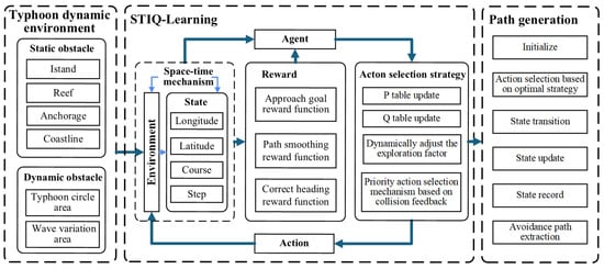
Figure 1.
Method framework.
2.3.1. STIQ-Learning Model
Based on the Markov decision process (MDP) [23,24], this paper integrates a spatio-temporal mechanism to propose the STIQ-Learning model. By incorporating the number of steps taken by the agent into the finite state set S, it enables the agent to distinguish between states with the same position/pose but different step counts, thereby receiving corresponding differentiated rewards to adapt to the dynamic obstacle environment. The algorithm’s objective is for the agent to find the optimal policy during training to maximize the cumulative reward. We assume the vessel moves at a constant speed, such that the number of steps reflects the time elapsed by the agent.
After integrating the spatio-temporal mechanism, the agent’s state space is defined by its longitude and latitude coordinates, heading, and step count, and is given by
where x, y, and are, respectively, the vessel’s longitude, latitude, and heading, forming the pose set C; and T is the agent’s step count set, which reflects the time elapsed for the vessel to reach a particular pose state.
In order to make the vessel’s turning angle closer to actual vessel motion, this paper designs and constrains the vessel’s turning angle based on experience. The vessel’s turning angle is discretized into a set of five discrete actions within the range of relative to the current heading:
With the integration of the spatio-temporal mechanism, the reward function R and cumulative return function G are related to the agent’s pose, the step count to reach the pose, and the chosen action, and can be expressed as
To maximize the cumulative reward, we define the state-value function and the action-value function. The state-value function is defined as the expected cumulative return of executing various actions according to a policy in a state , and its computational model after spatio-temporal integration is given by
The action-value function is defined as the expected cumulative return of executing a specific action according to a policy in a state , and its computational model after spatio-temporal integration is given by
2.3.2. Prior Knowledge-Based Reward Function Design
The objective of reinforcement learning algorithms is to enable the agent to maximize cumulative rewards through continuous interaction with the environment, progressing from the initial state to the target state. Consequently, the design of an appropriate reward function is critical, as informative and well-structured reward signals significantly enhance the agent’s ability to learn and adapt to the dynamics of the environment.
In this study, a set of sub-reward functions is designed to guide the agent toward generating trajectories that are goal-oriented, smooth, and compliant with the maneuverability constraints of ships. These sub-reward components provide targeted feedback to encourage desirable behaviors during the learning process. The specific sub-reward functions are defined as follows:
- (1)
- Approach Goal Reward FunctionTo guide the vessel toward the target point, avoid obstacles, and promote the selection of the shortest path, this paper defines a reward function in which actions that reach or approach the target receive a positive reward from the environment. Conversely, actions that result in collisions with obstacles or cause the vessel to deviate from the target are penalized with a negative reward. The reward calculation function is defined as
- (2)
- Path Smoothing Reward FunctionTo encourage the vessel to minimize unnecessary course changes during navigation and to ensure that the planned typhoon avoidance path remains as smooth as possible, this paper defines a reward function based on heading variation. Specifically, actions that result in smaller changes in heading angle between consecutive states receive higher positive rewards from the environment. The corresponding calculation function is defined aswhere and are, respectively, the vessel’s heading at the current time step and the next time step.
- (3)
- Correct Heading Reward FunctionTo encourage the vessel to align its heading toward the target point during the approach process, in accordance with typical navigational behavior, this paper defines a heading alignment reward function as follows:where is the bearing from the vessel’s position at the next time step to the target point’s position.
By taking a weighted summation of the sub-reward functions, the final reward function is constructed to comprehensively account for multiple objectives, including goal-directed navigation, trajectory smoothness, and heading alignment. The overall reward function is defined as
To enable the algorithm to dynamically adjust its weighting parameters in response to environmental changes, this study introduces a weight adaptation mechanism based on a multi-criteria priority structure. The mechanism monitors the average value of each sub-reward over a defined time period and compares it against predefined threshold values. Based on this comparison, the weight assigned to each sub-reward is adaptively adjusted according to its relative performance. The corresponding formulation is given as follows:
Here, , , and represent the average values of the three sub-rewards during the previous episode, while , , and denote the predefined threshold values for the corresponding sub-rewards. The parameter denotes the weight adjustment step size. The priority of the three rewards, from highest to lowest, is as follows: approach goal reward, path smoothing reward, and correct heading reward.
To ensure non-negativity and maintain the validity of the weight values, the updated weights are normalized at the final stage of the adjustment process.
2.3.3. Priority-Based Adaptive Action Selection Strategy
The -greedy strategy is a widely used action selection mechanism in reinforcement learning. At each time step, the agent selects the currently known optimal action with probability , and a random action with probability . While this strategy is straightforward to implement, it suffers from several limitations, including the following:
- (1)
- In most cases, is assigned a fixed value throughout the training process. This static setting lacks flexibility in balancing exploration and exploitation, as it fails to accommodate the agent’s need for extensive exploration in the early stages and efficient exploitation of learned knowledge in the later stages.
- (2)
- In the early stage of training, the agent requires extensive exploration due to the lack of prior knowledge. However, the limited number of training episodes and the absence of environmental information often lead to frequent collisions with obstacles, causing premature termination of episodes and thereby limiting the depth of environmental exploration. Meanwhile, during the initial phase of random exploration, the probability of selecting previously chosen actions is equal to that of unchosen actions, which restricts the breadth of exploration.
To address the aforementioned issues, building upon the -greedy strategy, this paper proposes a novel priority-based adaptive action selection strategy.
For the issue (1), this paper sets as a function that gradually changes with the number of successful episodes, and its value is given by
where is the initial exploration factor, and is the number of times the agent successfully reaches the target point. In the early stage of the algorithm, when the count of successful episodes is low, the agent is more inclined towards environmental exploration. As the agent interacts with the environment and the count of successful episodes increases, the algorithm favors exploiting prior knowledge to select the currently known optimal action, thereby achieving the adaptive adjustment of the exploration factor .
For the issue (2), this paper modifies the collision handling: the agent’s state is reset to the previous step upon collision with an obstacle, and the iteration is terminated only when the agent exceeds the effective map boundary. This encourages deeper environmental exploration during initial training. Simultaneously, a P table representing action selection probability is introduced alongside the Q table representing action values. After the agent executes an action, the following rules apply: ① If the next state results in a collision with an obstacle, the action priority becomes the lowest, and the probability of selecting this action in the future is set to 0. ② If all action selection probabilities in the next state are 0, the situation is treated equivalently to case ①. ③ If the next state does not result in a collision, the sampling priority of the action decreases with increasing sampling count. The priority is defined as
where n represents the selection count for this action, and the next selection probability is given by
where k is the size of the action set, and is the priority of this action. This mechanism encourages the agent to avoid repeatedly colliding with the same obstacle during the early exploration phase and promotes the selection of less frequently sampled actions, thereby enhancing the breadth of the agent’s environmental exploration.
2.3.4. Typhoon Avoidance Path Generation Process
After sufficient training, the Q-table gradually converges. Once convergence is achieved, the optimal path for the vessel from the initial position to the target can be determined based on the Q-values. Starting from the initial state, the agent selects the action with the highest Q-value at each step until the target position is reached. The sequence of longitude and latitude coordinates corresponding to the visited grid cells constitutes the planned typhoon avoidance path. The specific path generation process is shown in Figure 2.
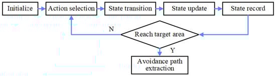
Figure 2.
Typhoon avoidance path generation flowchart.
- (1)
- Initialize: Execution starts from the initial state , and the state sequence is initialized.
- (2)
- Action Selection: In the current state , based on the converged Q-table, the action with the maximum Q-value is selected.
- (3)
- State Transition: After executing action , the agent transitions to the next state , which is given bywhere is the state transition function, representing the state reached after executing action a in state S.
- (4)
- State Update: is set as the new .
- (5)
- State Record: Add the state to the path sequence, and repeat steps (2) through (5) until the longitude and latitude of are within the target area.
- (6)
- Path Extraction: Each state in the state sequence is a multi-dimensional vector. To meet the requirements for visualization and practical application, the longitude and latitude coordinates are extracted from the path.
By following steps (1) through (6) above, the typhoon avoidance path from the initial point to the target point can be directly extracted from the well-trained Q-table.
3. Experiment and Analysis
3.1. Experimental Comparison and Analysis in a Grid Map Environment
To evaluate the performance of the proposed algorithm, simulation experiments were conducted in a grid-based environment. The STIQ-Learning algorithm was compared with several representative reinforcement learning-based path planning methods. The parameter settings used in the simulation experiments are summarized in Table 1.

Table 1.
Experimental parameter settings in the simulation environment.
In the simulation environment, blue regions indicate dynamic obstacle movement areas, yellow blocks represent dynamic obstacles, and black blocks denote static obstacles. The benchmark methods used for comparison include the conventional Q-Learning (CQL) algorithm, the Dynamic and Fast Q-Learning (DFQL) algorithm proposed in reference [16], and the proposed STIQ-Learning algorithm. Each algorithm is applied to generate a collision-free path from the starting point to the destination under the same map configuration. The resulting path planning outcomes are illustrated in Figure 3.
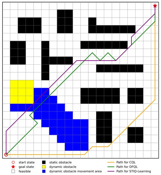
Figure 3.
Path planning results of different algorithms.
Since the results obtained from each experiment may vary, each algorithm is executed 20 times under identical environmental conditions. For each run, the path length and computation time are recorded, and their average values are calculated. The averaged results are summarized in Table 2.
Table 2.
Comparison between STIQ-Leaning, DFQL, and CQL.
By combining the data from Table 2 with the data from Figure 3, it can be observed that the proposed algorithm outperforms the CQL and DFQL algorithms in terms of both path length and computation time. In 20 repeated tests, STIQ-Learning achieves a 4.5% and 13.9% reduction in path length compared to DFQL and CQL, respectively, and a 1.63% and 7.52% reduction in computation time, respectively, bringing the generated paths closer to the global optimal path.
3.2. Experimental Comparison and Analysis in Typhoon Environment
In the experiments, the marine grid field is based on the forecast data provided by the European Centre for Medium-Range Weather Forecasts (ECMWF) [25]. To align with practical meteorological navigation scenarios, the data were interpolated to a spatial resolution of . For typhoon track and intensity information, subjective forecast data from the Central Meteorological Observatory were used. Since both the ECMWF forecast field and the typhoon forecast data were provided at 1-h intervals, the vessel’s position was estimated at the same temporal resolution during the experiments. This study considers only a constant-speed, variable-heading typhoon avoidance scheme.
3.2.1. Typhoon Example and Route Overview in Open Sea Areas
In order to verify the path generation performance of the STIQ-Learning algorithm for typhoon avoidance in open sea areas, this section takes Typhoon Pulasan (No. 14 in 2024) as the study subject. The typhoon entered the 24-h alert zone at 02:00 on 19 September 2024 (UTC+8; all times hereafter are in UTC+8), affecting the waters of the East China Sea. By 08:00 on the same day, its intensity had reached the level of a severe tropical storm, with a Beaufort 7 wind circle radius of 160 km. The typhoon moved in a northwesterly direction and made landfall in Zhoushan City, Zhejiang Province, China, at 18:00 on 19 September. This study focuses exclusively on the typhoon’s impact on vessels during its offshore phase, prior to landfall.
Taking a fully loaded bulk carrier navigating near the Chinese coast as an example, at 07:00 on 19 September 2024, the vessel was located at 122.4° E, 27.2° N, with a heading of 90°. Its destination was set to 124.4° E, 30.4° N. The vessel’s main characteristics include a molded depth of 13.5 m, a design draft of 10.5 m, a maximum tolerable wave height of 3 m, a maximum tolerable wind force of Beaufort scale 7, and a design cruising speed of 12 knots. Figure 4 illustrates the vessel’s originally planned route and the corresponding typhoon encounter scenario. The left panel displays a global satellite image, with a red box indicating the vessel’s navigation area. The right panel provides an enlarged view of the navigation region, where the black solid line represents the typhoon’s track, the red dashed line denotes the vessel’s planned trajectory, and Points A and B correspond to the departure and destination locations, respectively. The red circle marks the typhoon’s Beaufort 7 wind circle. If the vessel were to proceed along its original route, it would, according to the initial meteorological forecast, enter the Beaufort 7 wind circle at the point marked “X” in the right-hand panel of the figure, at approximately 14:00 on 19 September 2024.
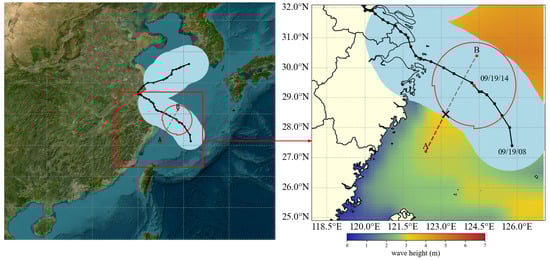
Figure 4.
Original planned route and typhoon encounter scenario in open sea areas.
3.2.2. Typhoon Avoidance Route Design in Open Sea Areas
To verify the effectiveness of the typhoon avoidance path generated by the proposed method in open sea areas, the typhoon avoidance route generated by the STIQ-Learning method is compared with the original planned route between the starting and ending points under the scenario described in Section 3.2.1.
Figure 5a–f illustrate the hourly segments of the typhoon avoidance route during the period when the vessel would potentially encounter the typhoon’s Beaufort 7 wind circle, spanning from 14:00 to 19:00 on 19 September 2024. In each subfigure, the background depicts the spatial distribution of effective wave height on the sea surface at the end time of the corresponding segment, where darker colors indicate higher wave heights. The red trajectory represents the originally planned route, while the blue trajectory indicates the optimized typhoon avoidance route. Point A marks the departure location and Point B denotes the destination. The red circles indicate the position of the Beaufort 7 wind circle at each time step. As shown in Figure 5, the original planned route leads the vessel into the Beaufort 7 wind circle starting at 14:00 on 19 September 2024, and keeps it within the hazardous zone for several subsequent hours (see Figure 5a–e). In contrast, the avoidance route generated by the STIQ-Learning method, which initiates an early constant-speed, variable-heading maneuver, successfully steers the vessel away from the hazardous region, keeping it consistently within the safe wave zone, indicated by the green-colored areas.
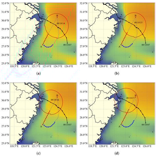
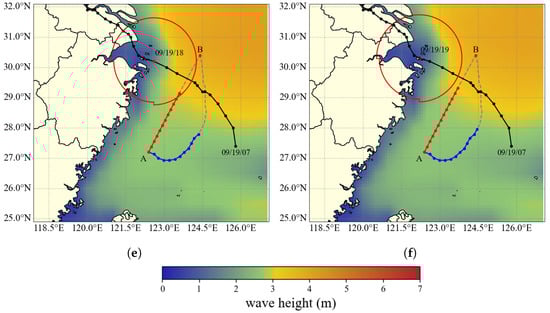
Figure 5.
Typhoon avoidance route and effective wave height distribution. (a) Route segment 1 (09/19/14:00). (b) Route segment 2 (09/19/15:00). (c) Route segment 3 (09/19/16:00). (d) Route segment 4 (09/19/17:00). (e) Route segment 5 (09/19/18:00). (f) Route segment 6 (09/19/19:00).
To further assess navigational safety, this study conducts a time-series comparison of the distance between the vessel and the typhoon center, as well as the effective wave height encountered along the two routes. The results are presented in Figure 6. In the figure, the red curve represents the original planned route, while the blue curve corresponds to the typhoon avoidance route generated by the STIQ-Learning algorithm. According to forecast data, Typhoon Pulasan’s Beaufort 7 wind circle has a radius of 160 km. Figure 6a compares the vessel-to-typhoon center distance. The minimum distance for the original planned route is 134.39 km, while that for the avoidance route is 259.97 km. These results demonstrate that the avoidance route effectively maintains a safe buffer outside the Beaufort 7 wind circle, thereby preventing the vessel from entering the hazardous zone. Figure 6b presents the comparison of effective wave height. The maximum wave height encountered along the original planned route is 3.29 m, whereas the maximum value for the avoidance route is 2.99 m. Considering the vessel’s structural characteristics described in Section 3.2.1, including a molded depth of 13.5 m and a design draft of 10.5 m, these results indicate that the avoidance route consistently keeps the vessel within a safer sea state.
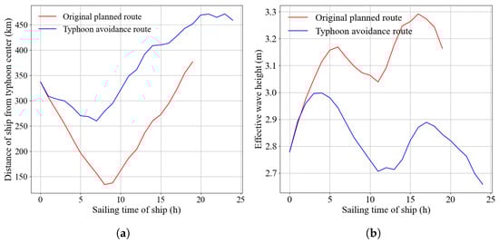
Figure 6.
Comparison of route information. (a) Vessel-to-typhoon distance comparison. (b) Effective wave height comparison.
3.2.3. Typhoon Example and Route Overview in Complex Sea Areas
To evaluate the performance of the STIQ-Learning algorithm in generating typhoon avoidance routes within complex maritime environments containing islands, this study selects Typhoon Gamei (No. 03 in 2024) as a representative case. The typhoon entered the 24-h warning zone at 17:00 on 23 July 2024, passed over Taiwan Island, and subsequently impacted the East China Sea. By 00:00 on 25 July 2024, Gamei had intensified into a strong tropical storm and approached the Taiwan Strait, exhibiting a Beaufort 10 wind circle with a radius of 70 km and following a northwestward trajectory.
Taking a fully loaded bulk carrier operating in China’s offshore waters as an example, at 03:00 on 25 July 2024, the vessel was located at 119.2° E, 23.5° N, with its bow oriented due north. The intended destination was 121.9° E, 25.8° N. The vessel’s specifications are as follows: a molded depth of 16.5 m, a design draft of 10.5 m, a maximum tolerable wave height of 6 m, a maximum tolerable sea surface wind force of Beaufort scale 10, and a design cruising speed of 12 knots. Figure 7 shows the vessel’s planned route and the forecasted typhoon impact. The left panel provides a global satellite view with a red box indicating the navigation area. The right panel enlarges this region, where the black line traces the typhoon’s path, the red dashed line shows the vessel’s planned trajectory, and Points A and B mark the departure and destination. The red circle denotes the Beaufort 10 wind circle at that time. According to the initial meteorological forecast, if the vessel were to continue along its original route, it would enter the Beaufort 10 wind circle at the location marked “X” in the right-hand panel of the figure, at approximately 09:00 on 25 July 2024.
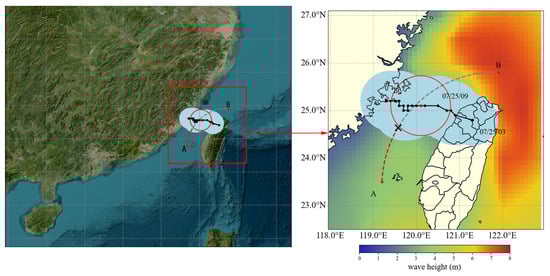
Figure 7.
Original planned route and typhoon encounter scenario in complex sea areas.
3.2.4. Typhoon Avoidance Route Design in Complex Sea Areas
To verify the effectiveness of the proposed method in generating typhoon avoidance routes within complex maritime environments, the comparative experiments described in Section 3.2.2 were repeated under the scenario outlined in Section 3.2.3. In contrast to the experimental setup in Section 3.2.2, which considered only wave height and wind fields, the current experiment incorporates islands as static obstacles, thereby increasing the environmental complexity and navigational constraints.
Figure 8a–f illustrate the segmented typhoon avoidance routes at hourly intervals from 09:00 to 19:00 on 25 July 2024. In each subfigure, the red trajectory represents the originally planned route, while the blue trajectory corresponds to the optimized typhoon avoidance route. Point A marks the departure location, and Point B indicates the destination. The red circles denote the position of the Beaufort 10 wind circle at each time step. If the vessel were to follow the original route, it would enter the Beaufort 10 wind circle at 09:00 on 25 July 2024. In contrast, the avoidance route involves a speed-preserving course adjustment strategy, which enables the vessel to steer clear of the hazardous wind zone while maintaining safe operational conditions.
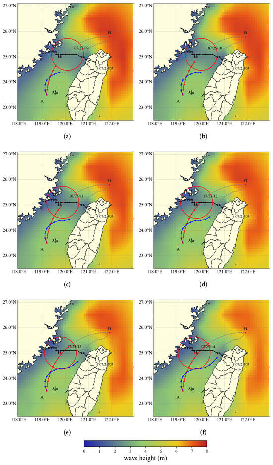
Figure 8.
Typhoon avoidance route and effective wave height distribution. (a) Route segment 1 (07/25/09:00). (b) Route segment 2 (07/25/10:00). (c) Route segment 3 (07/25/11:00). (d) Route segment 4 (07/25/12:00). (e) Route segment 5 (07/25/13:00). (f) Route segment 6 (07/25/14:00).
Figure 9 presents a time-series comparison of the distance between the vessel and the typhoon center, as well as the significant wave height encountered along the two routes. The red curve represents the original planned route, while the blue curve corresponds to the typhoon avoidance route. According to the forecast information for Typhoon Gamei, the radius of its Beaufort 10 wind circle is 70 km. In Figure 9a, the comparison of distances to the typhoon center reveals that the minimum distance between the original route and the typhoon center is only 15.15 km. In contrast, the avoidance route effectively maintains a safe separation from the hazardous wind zone, thereby preventing the vessel from entering high-risk areas that the original route would encounter. Meanwhile, in Figure 9b, the typhoon avoidance route is exposed to lower wave heights than the original planned route for most of the time and consistently remains within a relatively safe wave height range.
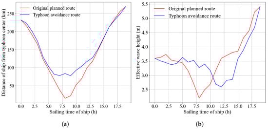
Figure 9.
Comparison of route information. (a) Vessel-to-typhoon distance comparison. (b) Effective wave height comparison.
3.2.5. Comparative Analysis of Different Path Planning Algorithms Under Typhoon Conditions
To verify the effectiveness of the proposed route optimization approach, path planning was conducted under the scenarios described in Section 3.2.1 and Section 3.2.3 using the STIQ-Learning method, as well as the DFQL, RRT, and D* algorithms. The resulting routes were evaluated based on three metrics: total path length, number of sharp turns, and number of 90° turns. The experimental parameter settings are provided in Table 3. The generated typhoon avoidance routes and corresponding quantitative results are presented in Figure 10 and Table 4, respectively. In these experiments, a sharp turn is defined as any turning angle exceeding 20° or falling below –20°.
Table 3.
Experimental parameter settings in marine environment.
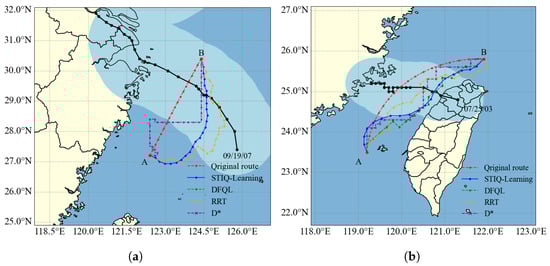
Figure 10.
Results of four methods for typhoon avoidance route planning. (a) Results in open sea areas. (b) Results in complex sea areas.
Table 4.
Comparison of typhoon avoidance routes.
Figure 10 shows the originally planned route (in red), along with the typhoon avoidance routes generated by the DFQL algorithm (green), the RRT algorithm (orange), the D* algorithm (purple), and the proposed STIQ-Learning method (blue).
Among the compared methods, the DFQL algorithm focuses on goal convergence and tends to steer directly toward the target point in open sea environments. However, in this scenario, where the vessel’s maximum tolerable wave height is limited to 3 m, the agent frequently collides with dynamic obstacles formed by hazardous wave regions in the early training phase. These repeated collisions lead to episode termination, hinder learning efficiency, and ultimately prevent the algorithm from producing valid avoidance routes. The D* algorithm prioritizes minimizing path length and tends to generate routes aligned with grid boundaries, resulting in unnatural right-angled turns and poor trajectory smoothness. The RRT algorithm, based on a random sampling strategy, adopts an “exploration-first” approach, which often leads to highly tortuous and non-smooth trajectories.
Table 4 presents a detailed comparison of the typhoon avoidance routes generated under different experimental conditions. The routes produced by the DFQL and D* algorithms contain multiple 90° sharp turns, which are impractical for real-world vessel maneuvering. Although the RRT algorithm avoids 90° turns, it still includes several sharp turns at other angles, compromising route smoothness.
In contrast, the proposed STIQ-Learning method consistently produces the shortest and smoothest routes across various scenarios, demonstrating better adherence to ship maneuverability constraints. These results indicate that under typhoon conditions, the STIQ-Learning method is both feasible and superior to the DFQL, D*, and RRT algorithms in generating safe and practical typhoon avoidance routes.
4. Conclusions
Existing ship path planning methods often face significant challenges in dynamic environments such as typhoons. These challenges include difficulties in accurately representing the continuous evolution of dynamic obstacles and the absence of adaptive exploration mechanisms. As a result, the generated paths are frequently suboptimal and may even violate fundamental ship maneuvering constraints.
To address these issues, this paper proposes the STIQ-Learning algorithm for dynamic typhoon avoidance path planning. First, the spatio-temporal environment is modeled based on forecast data. A spatio-temporal dynamic obstacle model was constructed by integrating wind circle radius and wave height forecast data, thereby capturing the continuous evolution of the typhoon. Then, by incorporating a state space extended with the time dimension and a compound reward mechanism comprising goal convergence, trajectory smoothness, and heading correction, the agent was guided to generate safe and efficient paths. Furthermore, a priority-based adaptive exploration strategy was introduced, which leverages collision feedback to enhance early-stage exploration efficiency and effectively balance the trade-off between exploration and exploitation, thereby mitigating the risk of falling into local optima. Finally, simulation experiments were conducted using Typhoons Pulasan and Gamei (2024) as case studies to validate the effectiveness and robustness of the proposed method under both open sea and island-constrained maritime scenarios.
The final results demonstrate that in open sea environments, the STIQ-Learning algorithm achieves route length reductions of 14.4% and 22.3% compared to the D* and RRT algorithms, respectively. In maritime areas with complex geographic features such as islands, the STIQ-Learning algorithm also outperforms the DFQL, D*, and RRT algorithms, reducing route lengths by 2.1%, 20.7%, and 10.6%, respectively. Moreover, the routes generated by the proposed method effectively eliminate sharp turns and consistently avoid hazardous wind zones throughout the voyage. As a result, the effective wave heights encountered remain below the vessel’s safety threshold, further ensuring navigational safety and operational feasibility under typhoon conditions.
By holistically accounting for the continuous evolution of the typhoon system, the proposed method generates routes that are not only shorter and smoother than those produced by traditional algorithms, but also more effective in avoiding hazardous typhoon zones. These improvements bring the resulting paths closer to the global optimum and highlight the method’s strong potential for real-world engineering applications.
To further enhance the practicality of typhoon avoidance path planning, future research may focus on incorporating fuel consumption considerations into the optimization process. Additionally, dynamically updating the planning scheme based on real-time forecast data could be explored to achieve a more adaptive and optimal typhoon avoidance strategy.
Author Contributions
Conceptualization and methodology, W.W.; Writing—original draft and visualization, F.L.; Investigation and Validation, K.C. and Z.N.; Supervision and writing—review and editing, Z.H. All authors have read and agreed to the published version of the manuscript.
Funding
This research is supported by Key Research and Development Project of Hubei Province, China (NO. 2023BAB013), National key research and development program (2023YFC3107904).
Data Availability Statement
The original data presented in the study are openly available in ECMWF website at https://doi.org/10.21957/open-data (accessed on 1 April 2025).
Conflicts of Interest
Authors Weizheng Wang, Kai Cheng and Zuopeng Niu are from the company. The authors declare no conflicts of interest.
References
- Feng, C.; Qin, T.; Ai, B.; Ding, J.; Wu, T.; Yuan, M. Dynamic typhoon visualization based on the integration of vector and scalar fields. Front. Mar. Sci. 2024, 11, 1367702. [Google Scholar] [CrossRef]
- Xu, B. Precise path planning and trajectory tracking based on improved A-star algorithm. Meas. Control 2024, 57, 1025–1037. [Google Scholar] [CrossRef]
- Huang, J.; Chen, C.; Shen, J.; Liu, G.; Xu, F. A self-adaptive neighborhood search A-star algorithm for mobile robots global path planning. Comput. Electr. Eng. 2024, 123, 110018. [Google Scholar] [CrossRef]
- Zhang, Z.; Wu, J.; Dai, J.; He, C. A Novel Real-Time Penetration Path Planning Algorithm for Stealth UAV in 3D Complex Dynamic Environment. IEEE Access 2020, 8, 122757–122771. [Google Scholar] [CrossRef]
- Kadry, S.; Alferov, G.; Fedorov, V.; Khokhriakova, A. Path optimization for D-star algorithm modification. Aip Conf. Proc. 2022, 2425, 080002. [Google Scholar]
- Yu, J.; Yang, M.; Zhao, Z.; Wang, X.; Bai, Y.; Wu, J.; Xu, J. Path planning of unmanned surface vessel in an unknown environment based on improved D* Lite algorithm. Ocean. Eng. 2022, 266, 112873. [Google Scholar] [CrossRef]
- Lin, Z.; Lu, L.; Yuan, Y.; Zhao, H. A novel robotic path planning method in grid map context based on D* lite algorithm and deep learning. J. Circuits Syst. Comput. 2024, 33, 2450057. [Google Scholar] [CrossRef]
- Meng, B.H.; Godage, I.S.; Kanj, I. RRT*-based path planning for continuum arms. IEEE Robot. Autom. Lett. 2022, 7, 6830–6837. [Google Scholar] [CrossRef]
- Fu, S. Robot Path Planning Optimization Based on RRT and APF Fusion Algorithm. In Proceedings of the 2024 8th International Conference on Robotics and Automation Sciences (ICRAS), Tokyo, Japan, 21–23 June 2024; pp. 32–36. [Google Scholar]
- Chen, G.; Luo, N.; Liu, D.; Zhao, Z.; Liang, C. Path planning for manipulators based on an improved probabilistic roadmap method. Robot.-Comput.-Integr. Manuf. 2021, 72, 102196. [Google Scholar] [CrossRef]
- Jamshidi, A.; Khanmirza, E. Improved Probabilistic Roadmap Path Planning Algorithm. In Proceedings of the 2024 12th RSI International Conference on Robotics and Mechatronics (ICRoM), Tehran, Iran, 17–19 December 2024; pp. 362–367. [Google Scholar]
- Yang, H.; Xu, X.; Hong, J. Automatic parking path planning of tracked vehicle based on improved A* and DWA algorithms. IEEE Trans. Transp. Electrif. 2022, 9, 283–292. [Google Scholar] [CrossRef]
- Wang, Y.; Fu, C.; Huang, R.; Tong, K.; He, Y.; Xu, L. Path planning for mobile robots in greenhouse orchards based on improved A* and fuzzy DWA algorithms. Comput. Electron. Agric. 2024, 227, 109598. [Google Scholar] [CrossRef]
- Wang, D.; Chen, H.; Lao, S.; Drew, S. Efficient path planning and dynamic obstacle avoidance in edge for safe navigation of USV. IEEE Internet Things J. 2023, 11, 10084–10094. [Google Scholar] [CrossRef]
- Wang, J.; Zhu, S.y.; Wang, G.z.; Wang, M.r. Route Optimization of Ship Avoiding Typhoon Under Meteorological Uncertainty. J. Dalian Marit. Univ. 2021, 47, 56–62. [Google Scholar]
- Hao, B.; Du, H.; Yan, Z. A path planning approach for unmanned surface vehicles based on dynamic and fast Q-learning. Ocean. Eng. 2023, 270, 113632. [Google Scholar] [CrossRef]
- Low, E.S.; Ong, P.; Low, C.Y. A modified Q-learning path planning approach using distortion concept and optimization in dynamic environment for autonomous mobile robot. Comput. Ind. Eng. 2023, 181, 109338. [Google Scholar] [CrossRef]
- Wang, Y.; Lu, C.; Wu, P.; Zhang, X. Path planning for unmanned surface vehicle based on improved Q-Learning algorithm. Ocean. Eng. 2024, 292, 116510. [Google Scholar] [CrossRef]
- Zhong, Y.; Wang, Y. Cross-regional path planning based on improved Q-learning with dynamic exploration factor and heuristic reward value. Expert Syst. Appl. 2025, 260, 125388. [Google Scholar] [CrossRef]
- Taskar, B.; Sasmal, K.; Yiew, L.J. A case study for the assessment of fuel savings using speed optimization. Ocean. Eng. 2023, 274, 113990. [Google Scholar] [CrossRef]
- Wang, J.; Wu, M. Descriptive Methodology for Risk Situation of Disastrous Sea Waves in the China Sea. J. Mar. Sci. Eng. 2025, 13, 188. [Google Scholar] [CrossRef]
- Carstens, J.D.; Didlake, A.C., Jr.; Zarzycki, C.M. Tropical Cyclone Wind Shear-Relative Asymmetry in Reanalyses. J. Clim. 2024, 37, 5793–5816. [Google Scholar] [CrossRef]
- Sutton, R.S.; Barto, A.G. Reinforcement Learning: An Introduction; MIT Press: Cambridge, UK, 1998. [Google Scholar]
- Chen, C.; Chen, X.Q.; Ma, F.; Zeng, X.J.; Wang, J. A knowledge-free path planning approach for smart ships based on reinforcement learning. Ocean. Eng. 2019, 189, 106299. [Google Scholar] [CrossRef]
- Sasa, K.; Chen, C.; Fujimatsu, T.; Shoji, R.; Maki, A. Speed loss analysis and rough wave avoidance algorithms for optimal ship routing simulation of 28,000-DWT bulk carrier. Ocean. Eng. 2021, 228, 108800. [Google Scholar] [CrossRef]
Disclaimer/Publisher’s Note: The statements, opinions and data contained in all publications are solely those of the individual author(s) and contributor(s) and not of MDPI and/or the editor(s). MDPI and/or the editor(s) disclaim responsibility for any injury to people or property resulting from any ideas, methods, instructions or products referred to in the content. |
© 2025 by the authors. Licensee MDPI, Basel, Switzerland. This article is an open access article distributed under the terms and conditions of the Creative Commons Attribution (CC BY) license (https://creativecommons.org/licenses/by/4.0/).