A Time Synchronization Hop-Count-Control Algorithm Based on Synchronization Error Convergence Probability Estimation

Abstract

High-precision time synchronization is regarded as the foundation for ensuring the stable operation of microgrids and for the coordinated sensing, communication, and computing among network devices. In multi-hop wireless sensor networks, it is observed that both the accumulation of synchronization errors and the associated communication overhead are increased with the number of hops; however, in single-hop mode, it is found that the rate of error convergence is insufficient to satisfy the requirements for rapid synchronization. To address these challenges, a hop-control time synchronization algorithm based on the estimation of synchronization error convergence probability is proposed. In the proposed method, the convergence probability of the synchronization error at each node and its rate of change are estimated online, so that the synchronization hop count can be dynamically adjusted: during the synchronization establishment phase, a larger hop count is employed to accelerate error convergence; during the synchronization maintenance phase, the minimal hop count is utilized to maintain long-term high-precision synchronization, thereby ensuring synchronization accuracy and significantly reducing communication overhead. MATLAB simulation results are reported to have demonstrated that the proposed algorithm exhibits marked advantages in convergence speed, synchronization accuracy, and energy consumption as compared to fixed-hop-count and pure single-hop schemes, thereby providing an effective solution for efficient time synchronization in multi-hop wireless sensor networks.

1. Introduction

Traditional Phasor Measurement Unit (PMU) [1,2] technology in microgrids provides rapid synchronized measurements, ensuring stable operation of distribution networks [3,4]. However, in modern microgrids, where the diversity of Distributed Energy Resources (DERs), the integration of Energy Storage Systems (ESSs), and bidirectional energy flows are encountered, system equipment and communication networks are rendered exceptionally complex [5]. Under such circumstances, the application of conventional PMU technology is hindered by high costs, increased system complexity, and its reliance on external precise time sources such as the Global Positioning System (GPS) [6].

In response to these challenges, the introduction of wireless sensor network (WSN) time synchronization technology has been explored by researchers in recent years to address complex network issues and to reduce dependence on GPS technology, thereby alleviating both the economic and technical burdens of system implementation [7]. As time synchronization is regarded as a critical foundational technology for intelligent monitoring and control systems in microgrids, its application scope is considered to include, but is not limited to, real-time monitoring [8] and protection [9], energy management [10], and dispatch [11].

Currently, various time synchronization algorithms in WSNs have been widely investigated and are generally classified into three categories: centralized, semi-distributed, and distributed. Centralized algorithms, such as Reference Broadcast Synchronization (RBS) [12] and Timing-sync Protocol for Sensor Networks (TPSN) [13], are dependent on explicit topology management; however, in microgrid scenarios where nodes are loosely distributed and subject to frequent changes, high topology maintenance costs are incurred. Semi-distributed algorithms, such as the Flooding Time Synchronization Protocol (FTSP) [14], require the utilization of reference nodes rather than full topology management, yet network topology and routing conditions are found to affect their performance. Distributed algorithms, exemplified by Average Time Synchronization (ATS) [15] and Gradient Time Synchronization Protocol (GTSP) [16], do not rely on a fixed topology and are regarded as providing better adaptability and robustness, which facilitates high synchronization accuracy in complex distributed environments; however, a slower convergence speed is often observed with these algorithms.

The ATS algorithm, as a conventional distributed time synchronization method, has been widely applied in WSNs. In this approach, each node periodically averages its own clock with those of neighboring nodes through multiple iterations, thereby obtaining a unified clock. It is characterized by high accuracy and strong robustness; however, in complex networks, its convergence speed is slow, and in linear networks, achieving rapid error convergence within a short period is particularly challenging [17,18]. In contrast, the FTSP algorithm, which is categorized as a semi-distributed time synchronization method, relies on nodes periodically broadcasting local time messages that are subsequently relayed through a virtual hierarchical network to all nodes. The FTSP method is noted for its fast convergence of synchronization error and robust performance; nevertheless, it suffers from deteriorating accuracy as the network diameter increases due to the accumulation of synchronization errors along multi-hop paths [19,20].

It can be observed that various algorithms are affected by the actual network structure and scale in microgrids, with each offering distinct advantages and limitations in terms of synchronization precision, convergence speed, and communication overhead [21,22]. However, in practical applications, network topologies are complex and diverse, and existing time synchronization algorithms are often tailored to a single scenario, thus lacking effective adaptability [23]. The number of hops used for transmitting synchronization information is critical to algorithm performance: multi-hop communication results in behavior similar to FTSP, which achieves rapid convergence but is prone to cumulative errors, while single-hop communication results in behavior akin to ATS, which offers high precision but slow convergence. Therefore, it is necessary to develop a time synchronization algorithm that can autonomously adjust the hop count to suit different synchronization phases and network structures.

The Multi-Hop Average Consistency Time-Sync (MACTS) [24] algorithm is a multi-hop average consistency time synchronization scheme that enhances the network’s algebraic connectivity by establishing virtual links between nodes. It employs a multi-hop controller to balance convergence time, convergence precision, and communication complexity. In MACTS, hop count is adjusted via a preset synchronization error threshold: if the local convergence metric falls below this threshold, the hop count is decreased by one; if it exceeds the threshold, the hop count is increased by one—up to the initially configured maximum.

However, in real-world deployments, selecting an appropriate error threshold in advance is challenging. During the early application of time synchronization methods, users typically lack sufficient knowledge of the network’s topology and characteristics, making a global threshold difficult to set. Moreover, sensor networks vary widely in size, shape, and device specifications, so the precision achievable at each node differs; a single fixed threshold cannot accommodate such heterogeneity. Consequently, controlling hop count solely by a predetermined error threshold has inherent limitations.

In addition, the reliance of MACTS on a fixed initial hop count also poses practical difficulties. Under its control strategy, when the local synchronization error exceeds the preset threshold, the hop count increases—but cannot surpass the initial value, which thus becomes the algorithm’s maximum. In networks with random node numbers, densities, or topologies, it is impractical to choose a one-size-fits-all maximum hop count, further limiting adaptability for MACTS.

To address these issues, this paper integrates the Adaptive Real-time Convergence Estimation (ARCE) [25] algorithm to propose a hop-control time synchronization (HCTS) algorithm based on the estimated probability of synchronization error convergence. Our method continuously estimates the network’s convergence state from instantaneous synchronization errors and dynamically adjusts each node’s hop count according to this real-time convergence probability.

During the time synchronization establishment phase, the HCTS algorithm employs a multi-hop information transmission mode so that synchronization information is rapidly forwarded, thereby achieving rapid preliminary error convergence across all network nodes. After synchronization convergence has been achieved, the algorithm transitions into the synchronization maintenance phase, during which the hop count is gradually reduced as the system shifts to a single-hop time synchronization framework. This transition is intended to reduce synchronization overhead and achieve higher synchronization precision.

It is worth noting that the MACTS algorithm adjusts hop counts using a pre-defined synchronization error threshold; however, in dynamic or heterogeneous networks, a fixed threshold often fails to accommodate real-time error variations across nodes, resulting in suboptimal performance. In contrast, the HCTS algorithm proposed herein incorporates an online estimation of the synchronization error convergence probability and its rate of change, enabling real-time hop-count adjustments for finer-grained control of the synchronization process. This probability-driven mechanism not only accelerates error convergence and enhances synchronization accuracy, but also endows the algorithm with greater robustness and applicability in sensor networks exhibiting diverse accuracies, topologies, and node characteristics.

MATLAB simulations demonstrate that the algorithm jointly adjusts node hop count based on synchronization error convergence probability and its rate of change, improving synchronization precision and convergence speed while reducing communication overhead.

This article is organized into five sections. Section 1 is the introduction. Section 2 presents the system model, which defines the key components and parameters used in the proposed algorithm. Section 3 describes the algorithm design, including the ARCE convergence probability estimation and the hop-control mechanism. Section 4 reports the experimental simulation results, analyzing the synchronization error, hop control, and overall algorithm performance. Finally, Section 5 discusses the paper and concludes it.

2. System Model

The WSN is modeled as $\psi =(V,\epsilon )$, where the node is defined as $V=\{1,\dots ,N\}$. $\psi$ is a collection of $\epsilon$ edges, $\epsilon \subseteq \left\{\right(i,j):i,j\in V\}$, because it is an undirected graph $\psi$. $(i,j)$ refers to the edge connections between nodes $v_i$ and $v_j$, which can communicate with each other. We define the set of neighbors of node $v_i\in V$ as $N_i=\{v_i\in V:\{i,j\}\in \epsilon \}$.

2.1. Clock Model

The wireless sensor node controls the clock running rate with the counter and provides the clock source with the crystal oscillator. The nominal frequency of the crystal oscillator is expressed by f, while the actual frequency is expressed by $f_i$. In the clock model of the time synchronization algorithm, there are two types of clock: a hardware clock and logical clock. The mathematical model of the hardware clock is expressed as

$$H\left(t\right)={\int }_0^{t}h\left(\tau \right)d\tau$$

(1)

In Equation (1), $h\left(\tau \right)$ is the hardware frequency (clock speed) of the clock source and the inherent property of the crystal oscillator.

The mathematical model of logical clock is expressed as

$$L\left(t\right)=\phi \left(t\right)\times H\left(t\right)+\theta \left(t_0\right)$$

(2)

In Equation (2), $\phi \left(t\right)$ is the logical relative clock frequency multiplier, $\theta \left(t_0\right)$ is the initial relative clock offset, and $L\left(t\right)$ provides the global time service for synchronization applications in WSNs. We can further write the updated model of $L\left(t\right)$ as

$$L^{+}\left(t\right)=L\left(\tau \right)+(H\left(t\right)-H\left(\tau \right))\times {\phi }_i^j+{\theta }_i^j,(t>\tau )$$

(3)

where ${\phi }_i^j$ and ${\theta }_i^j$ are the relative clock offset and relative clock rate between any node $v_i$ and $v_j$, respectively. The two are respectively obtained by the following formulas:

$${\phi }_i^j={\displaystyle \frac{H_j\left(t\right)-H_j(t-\tau )}{H_i\left(t\right)-H_i(t-\tau )}},\tau >0$$

(4)

$${\theta }_i^j=L_j\left(t\right)-L_i\left(t\right)$$

(5)

2.2. Error Model

(1) Local synchronization error. The synchronization error between two adjacent nodes is called local synchronization error and is expressed as

$$E_l\left(t\right)={sup}_{i,j\in N_i}\{L_i\left(t\right)-L_j\left(t\right)\}$$

(6)

where nodes $v_i$ and $v_j$ are neighbors.

(2) Global synchronization error. The global synchronization error is used to describe the synchronization error between any node pair, expressed as

$$E_g\left(t\right)={sup}_{i,j\in N_i}\{L_i\left(t\right)-L_j\left(t\right)\}$$

(7)

where nodes $v_i$ and $v_j$ are not necessarily neighbors.

3. Implementation of HCTS

The HCTS can be divided into two main parts: the ARCE convergence probability estimation component and the step control component. The design flowchart is shown in Figure 1.

In the ARCE convergence probability estimation section, the synchronous error estimate is $E_l\left(k\right)$, obtained through the calculation of pairs of instantaneous timestamps with the ARCE algorithm, the statistical error $\mu$, the standard deviation of average $\sigma$, and computation and filtering of convergence probability estimates of the current output node ${\widehat{P}}_c$.

The control section contains three modules: (1) The synchronization information processing unit: This unit achieves convergence in the probability estimate ${\widehat{P}}_c$, using Exponentially Weighted Moving Average (EWMA) filter processing to obtain ${\widehat{P}}_E$. At the same time, the synchronous counter value M of the synchronization algorithm needs to be obtained. (2) Hop adjustment information processing unit: This unit computes the convergence-probability variation rate $\delta$ based on ${\widehat{P}}_E$ and M obtained from the preceding unit, and then incorporates ${\widehat{P}}_E$, M, and $\delta$ into the hop information matrix. (3) Hop adjustment unit: In this unit, error rate of change in the $\delta$ and the error convergence probability ${\widehat{P}}_E$ jointly determine the node hop to adjust. We need to compare the size of the convergence probability bound value $\xi$ and ${\widehat{P}}_E$, the size of the error probability in the convergence rate analysis of the current convergence situation, and then adjust and make the hop. After the new hop number is obtained, the new hop number is fed back to the time synchronization algorithm, and a new synchronization error is estimated to start a new cycle.

3.1. ARCE Algorithm

In this work, synchronization errors in the HCTS algorithm are treated by the ARCE algorithm. The local synchronous error estimate $E_l\left(k\right)$ is used as an input function to detect local convergence states, and, after being processed by a buffer unit, the convergence probability estimate ${\widehat{P}}_c$ is generated.

(1)

Convergence probability estimation

ARCE obtains the local synchronization error estimation $E_l\left(k\right)$ by paired timestamps, and calculates the mean value of error $\mu$ and standard deviation $\sigma$ by the synchronization error characteristic estimator after multiple statistics. At the same time, $E_l\left(k\right)$ is used as the input value, and the convergence probability value out is output by a three-stage function.

$$out=\left\{\begin{array}{cc}\hfill 0,& \mathrm{if}{E}_l\left(k\right)>E_{max}\hfill \\ \hfill a,& \mathrm{if}{E}_{max}\ge E_l\left(k\right)\ge \mu +3\sigma \hfill \\ \hfill 1,& \mathrm{if}{E}_l\left(k\right)<\mu +3\sigma \hfill \end{array}\right.$$

(8)

In Equation (8), $E_{max}$ represents the synchronization error threshold of the transition stage. By comparing the above equation, the error can be divided into three states: when the synchronization error estimate is greater than the maximum threshold, the output convergence probability is 0, which is not convergence. When the synchronization error estimation between the maximum threshold value and effective value is obtained, with an output convergence probability of a, considered the transition state, the $a\in (0,1)$. When the synchronization error estimate is less than the effective value, the output convergence probability is 1, indicating that the error has converged. In addition, a is the convergence–decision coefficient. When $a\to 1$, convergence is loose: the reliability and stability of $\mu$ and $\sigma$ decrease, while the convergence–decision rate increases. Conversely, when $a\to 0$, convergence is strict, and $\mu$ and $\sigma$ exhibit the opposite behavior. Therefore, when selecting an appropriate a, one must consider the convergence characteristics of the time synchronization algorithm.

The parameter $E_{\max }$ is a threshold for the transition phase of the time synchronization algorithm. The parameter $E_{\max }$ is set based on the accuracy of the time synchronization algorithm and the granularity of the clock source. For instance, if the accuracy of the time synchronization algorithm is about N ticks of the clock source, then $E_{\max }$ can be set to $m\times N(m>1)$ ticks, e.g., 200 µs. In addition, $E_{\max }$ can be updated in real time by using $\mu$ and $\sigma$, and is given by

$$E_{\max }=\rho \mu +\beta \sigma ,$$

(9)

where $\rho >1$ and $\beta >1$. In the following experiments and simulations, $\rho$ and $\beta$ are set to 2 and 3, respectively.

With each time synchronization, the mean value $\mu$ and standard deviation $\sigma$ of synchronization error will change due to the input of new data. Therefore, the existing mean value $\mu$ and standard deviation $\sigma$ need to be fed back to the synchronization error characteristic estimator for updating.

(2)

Buffer unit PU

Every time the convergence probability estimator completes an $E_l\left[k\right]$ convergence probability estimation, its output estimate is entered into the buffer PU cache. A first-in first-out storage unit with length $L_p$ is defined to store the convergence probability estimate of the output.

(3)

Convergence probability calculation

The convergence probability of the current time synchronization error is calculated by using a sample set in the buffer. A weighted average filter is used with the number of weighted coefficients $L_p$.

$${\widehat{P}}_c={\displaystyle \frac{\sum PU}{L_p}}$$

(10)

${\widehat{P}}_c$ is the error convergence probability, and $L_p$ is the depth of the PU, which can be understood as a buffer unit. $L_p$ values will affect the ${\widehat{P}}_c$ convergence rate and smoothness. The smaller the depth of the PU, ${\widehat{P}}_c$, the faster the convergence speed. The greater the depth of the PU, ${\widehat{P}}_c$, the slower the convergence speed, but the more stable. Therefore, depth can be set according to the requirements of different smoothness and sensitivity values in application.

3.2. Hop Control

In a multi-hop network, with an increase in the number of hops, the following situations will occur: First, the cumulative error on the multi-hop path will increase. Second, the amount of information will increase. Third, the probability of information collision will increase. Therefore, when the errors of the time synchronization algorithm have converged, reducing the hops of information transmission without affecting the convergence will greatly improve the above cases.

To overcome the above problems, a multi-hop controller is designed in this paper, as shown in Figure 2. The controller is divided into a synchronization information processing unit, a hop adjustment information processing unit, and a hop adjustment unit.

(1)

Synchronize the information processing unit

The synchronization information processing unit comprises three components: the ARCE algorithm, an EWMA filter, and a time synchronization acquisition module. First, the ARCE algorithm computes the error convergence probability ${\widehat{P}}_c$. This probability is then smoothed by an EWMA filter to estimate and stabilize network state parameters, eliminating short-term fluctuations. Its formula is as follows:

$${\widehat{P}}_E\left(t\right)=\lambda Y\left(t\right)+(1-\lambda ){\widehat{P}}_c(t-1),t=1,2,\dots ,L_p$$

(11)

In the equation for ${\widehat{P}}_E\left(t\right)$ time estimates, $\lambda$ is the smoothing factor, that is, the weight coefficient of the historical measurement value; $Y\left(t\right)$ is the t time measured value (in this article, the t moment convergence probability is an estimate of ${\widehat{P}}_c$). The closer the value of $\lambda$ is to 1, the lower the weight of the previous measured value, and the stronger the timeliness of the algorithm is. On the other hand, the size of $\lambda$ can also reflect the ability of the algorithm to absorb instantaneous emergencies. The smaller the value of $\lambda$, the stronger the stationarity.

The synchronization information processing unit also needs to obtain the synchronization count value M of the time synchronization algorithm. The first synchronization refers to the number of synchronizations from the first count. If it is the synchronization after the hops were adjusted, it refers to the number of synchronization counts since the hops were adjusted.

(2)

Hop adjustment information processing unit

After filtering, the convergence probability ${\widehat{P}}_E$ corresponds to a synchronous M, calculated with synchronous frequency, which increases convergence probability and the rate of change of $\delta$. The formula is as follows:

$${\delta }_a^b={\displaystyle \frac{{\widehat{P}}_{E_b}-{\widehat{P}}_{E_a}}{M_b-M_a}}$$

(12)

In Equation (11), a and b indicate the number of time synchronizations, and $b>a$. ${\delta }_a^b$ refers to the change rate of error convergence probability between the A-th synchronization and the B-th synchronization, which can be understood as the first derivative of error convergence change during the two synchronizations. When ${\delta }_a^b\ge 0$, the probability of error convergence increases during the two synchronization periods of a and b. When ${\delta }_a^b<0$, the probability of error convergence is in a declining trend during the two synchronization periods of a and b. The probability of convergence rate ${\delta }_a^b$, synchronous number M, and convergence probability estimate ${\widehat{P}}_c$ being in the hop adjustment coefficient matrix is shown in

Table 1. Hop-count adjustment information table.

Synchronization Time M	Probability Convergence ${\widehat{\mathit{P}}}_{\mathit{E}}$	Rate of Change $\mathit{\delta }$
$M_1$	${\widehat{P}}_{E_1}$	-
$M_2$	${\widehat{P}}_{E_2}$	${\delta }_1^2$
$M_3$	${\widehat{P}}_{E_3}$	${\delta }_2^3$
...	...	...
$M_n$	${\widehat{P}}_{E_n}$	${\delta }_{n-1}^n$

.

(3)

Hop adjustment unit

Adjusting hops by the error probability of convergence rate is the main task of the hop adjustment unit. $\delta$ and error convergence probability ${\widehat{P}}_E$ jointly determine the node hop to adjust. This unit accepts as inputs the filtered error-convergence probability estimate ${\widehat{P}}_E$ and its rate of change $\delta$, and produces one of three control actions: “reduce hops,” “maintain hops,” or “increase hops.”

The parameter $\xi$ is set to the convergent probability judgment limit, where $\xi \in (0,1)$. The limit value here can be adjusted flexibly with the required probabilistic judgment rigor, and the closer $\xi$ is to 1, the higher the requirement of convergence probability. $\eta$ is a regulating factor whose value is jointly determined by (i) the comparison between the filtered error-convergence probability estimate ${\widehat{P}}_E$ and the threshold $\xi$, and (ii) the rate of change $\delta$ of the error-convergence probability. The resulting $\eta$ is then used to adjust the hop count. Specific judgment methods are as follows:

$$\eta =\left\{\begin{array}{cc}\hfill -1,& {\widehat{P}}_E\ge \xi ,\delta \ge 0,\hfill \\ \hfill 0,& {\widehat{P}}_E\ge \xi ,\delta <0,\hfill \\ \hfill 0,& {\widehat{P}}_E<\xi ,\delta \ge 0,\hfill \\ \hfill 1,& {\widehat{P}}_E<\xi ,\delta <0.\hfill \end{array}\right.$$

(13)

When ${\widehat{P}}_E$ is greater than or equal to the specified convergence probability judgment limit value $\xi$, and the change rate of $\delta$ is greater than or equal to 0, it can be judged that the probability of error convergence at this time reaches the specified threshold and increases. Therefore, we assign −1 to the adjustment coefficient $\eta$, indicating that the node hops can be reduced by one hop.

Whether ${\widehat{P}}_E$ is greater than or equal to $\xi$ is deduced, and the rate of change in $\delta$ is less than 0, although convergence probability indicates that the threshold rate has dropped so it has not achieved stable convergence. The adjustment coefficient $\eta$ is set to 0, indicating that the number of hops remains unchanged.

When ${\widehat{P}}_E$ less than $\xi$ is deduced and the rate of change in the $\delta$ is greater than or equal to 0, although the probability rate is rising, the convergence probability still fails to reach the specified threshold; therefore, 0 is assigned to $\eta$ to maintain the original jump number.

When ${\widehat{P}}_E$ is less than $\xi$ and the rate of change in $\delta$ is less than 0, we can judge that the convergence of probability does not meet the prescribed threshold and continues to decline; therefore, assigning 1 to $\eta$ means that the number of node hops should increase by 1.

After adjusting the hop number, the adjusted hop number is fed back to the original time synchronization algorithm, related steps of time synchronization are re-performed to obtain new synchronization information, and then a new round of hop number adjustment is carried out. Under ideal conditions, all nodes can converge to one hop after adjusting the number of round hops.

The pseudo-code of HCTS is presented in Algorithm 1. After the broadcast task is triggered, it immediately begins to send time information packets $\langle H_i\left(t\right),L_i\left(t\right),{\phi }_i,H\rangle$ to neighboring nodes, which includes establishing two sets of time series $H_i\left(t\right)$ and $L_i\left(t\right)$ during the broadcast phase, relative to clock drift ${\phi }_i$ and the current running hop count of the node H. After the convergence rate estimation and parameter control calculation described above, the hop count of the new node undergoes a new round of time synchronization.

Algorithm 1: The pseudo-code of HCTS algorithm. The reference nodes are denoted as R, and the node under consideration is $i\in V$.

1  Initialization:  2     Set ${\phi }_i=1,{\phi }_i^j=1,{\theta }_i^j=0,H=5$  3     Set $H_{\mathit{i},\mathit{old}}=0,H_{\mathit{j},\mathit{old}}=0$  4     Set periodic task to broadcast, periodic task is set as B  5  When periodic task is broadcast:  6     Broadcast $\langle H_i\left(t\right),L_i\left(t\right),{\phi }_i,H\rangle$  7  Receive synchronization message $\langle H_j\left(t\right),L_j\left(t\right),{\phi }_j,H\rangle$:  8     Store received data: $\langle H_i\left(t\right),H_j\left(t\right)\rangle ,\langle L_i\left(t\right),L_j\left(t\right)\rangle ,{\phi }_j$  9     Compute ${\phi }_i^j,{\theta }_i^j,E_l\left(k\right),\mu ,\sigma$ 10   Compute ${\widehat{P}}_C,{\widehat{P}}_E,\gamma ,\delta$ 11   Update ${\phi }_i\leftarrow \langle {\phi }_i^j,{\phi }_i^j\rangle$, H

4. Experimental Simulation

In order to evaluate the performance of the proposed algorithm, all simulations were conducted on the MATLAB (R2016a) platform. The experimental design and subsequent result analyses were focused on three key metrics: synchronization error, hop count, and overall algorithmic performance. To ensure statistical significance and result stability, extensive repeated simulations were performed, with each configuration executed no fewer than 500 times. Statistical results were obtained from these simulation runs.

4.1. Error Analysis

In the grid network, the WSN was set as a 5 × 5 grid with a total of 25 nodes, and the diameter of the network was 8. We set 50 time synchronizations in one round of simulation, and each time synchronization period was 30 s. We collected statistics on local synchronization errors and global synchronization errors, and the results are presented in Figure 3.

Local synchronization error: In this simulation, the variation curve of the local synchronization error, $E_l$, for all nodes in the WSN was obtained. With an increasing number of synchronization events, M, the local synchronization error of each node was gradually reduced. Local error convergence was achieved for all nodes after the third synchronization cycle, with the convergence error remaining within 6 microseconds.

Global synchronization error: The variation trend of the global synchronization error, $E_g$, was found to be similar to that of the local synchronization error. Global error convergence was observed for all nodes between the 19th and 21st synchronization cycles, with the global error converging within 9 microseconds.

4.2. Hop-Control Analysis

This algorithm controls the hop count on the premise of achieving error convergence, and increases and decreases the hop count by estimating the convergence probability and statistics of the change rate of the time synchronization algorithm, so as to achieve an adaptive hop count.

In this experiment, the initial hop number of nodes in the 10 × 10 grid network is set to 7 hops, and the threshold value of parameter convergence probability judgment $\xi$ is 0.9 (the closer $\xi$ to 1, the higher the requirement of convergence probability), and the probability change rate $\delta$ is calculated. By comparison results from ${\widehat{P}}_E$ and $\xi$ and the factor of the comparison results, the error rate $\delta$ is used to adjust the hop. After synchronization convergence is achieved, the convergence probability approaches 1; a smaller rate of change at this point indicates a smoother convergence. Furthermore, the hop-count adjustment mechanism will progressively reduce the number of synchronization hops—ultimately decreasing to a single hop—thereby minimizing the overhead associated with multi-hop synchronization.

Figure 4 is an example of an arbitrarily selected node in the network. The effect of the rate of change and the probability of convergence on the change of node hops can be observed. When the convergence probability is greater than 0.9 and the change rate is greater than 0, the hop count decreases by one hop. When the convergence probability is less than 0.9 and the change rate is less than 0, the hop count increases by one hop. When the probability of convergence is greater than 0.9 but the rate of change is less than 0, or when the probability of convergence is less than 0.9 but the rate of change is greater than 0, the number node hops remains the same.

In order to observe the hop number change of all nodes in the whole network, we calculate the hop number change in a grid network of 10 × 10 with a synchronization period of 30 s and draw a statistical graph. As shown in Figure 5, all nodes have 7 hops at the beginning of synchronization, but the average number of hops gradually decreases with an increase in synchronization time. At the same time, it can be observed that the hop count of node 9 is not only reduced but the hop count of individual nodes will also fluctuate due to the impact of the synchronization error. The maximum hop count reaches 9 hops, but the final hop count will converge to 1 hop with the convergence of the error.

4.3. Algorithm Performance Comparison

Taking a 10 × 10 grid network as an example, comparative experiments were conducted under identical network scales and other synchronization parameters, in which the conventional ATS algorithm, the MACTS algorithm with an integrated multi-hop controller, and the proposed HCTS algorithm were evaluated. Figure 6 displays the convergence curves of the global error for the three algorithms.

As a time synchronization algorithm that transmits information with a single hop, the ATS algorithm has difficulty achieving error convergence in a short time in a large-scale network. As shown in the figure above, after 200 synchronization cycles, the ATS algorithm fails to achieve error convergence.

As a fast time synchronization error convergence algorithm, MACTS can quickly set the threshold range of error convergence values and maintain its convergence accuracy. The disadvantage of MACTS is that it uses a local convergence detector to directly determine whether hops are maintained or reduced based on a specified error. The judgment method is unique and the threshold is fixed. When the error is much larger or much smaller than the threshold, the judgment method will be invalid.

HCTS has obvious convergence characteristics: In the early stage, it uses multi-hop information transmission to carry out fast synchronization information forwarding, so it achieves fast convergence of synchronization errors in the time synchronization establishment stage. When the error converges gradually, the hop count decreases gradually. In order to obtain lower synchronization costs and higher synchronization accuracy, information transmission is carried out with a small hop count. As shown in Figure 6, the HCTS demonstrates advantages in both convergence speed and precision.

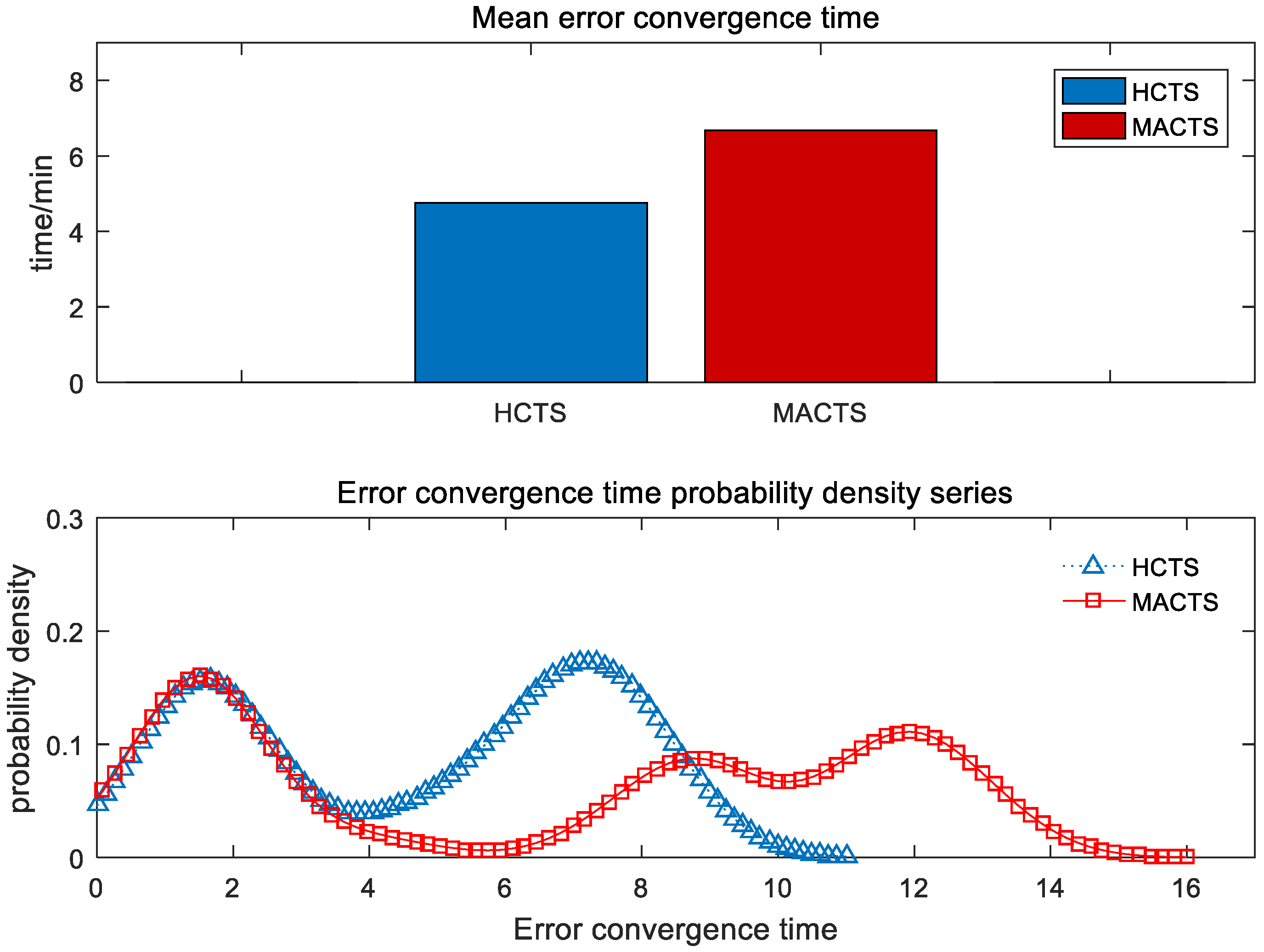
Using the global synchronization error as the comparison metric, multiple experiments were conducted in a 5 × 5 grid network to statistically analyze both the mean convergence time and the probability distribution of each node’s convergence time. The results are shown in Figure 7. A comparison of the two algorithms revealed that the proposed HCTS algorithm exhibited an average global error convergence time of 4.76 min, which was lower than the 6.68 min required by the MACTS algorithm. Moreover, the probability density plot indicated that the convergence time of the HCTS algorithm was more concentrated and stable. Consequently, under identical network parameters, the HCTS algorithm demonstrated both a faster average convergence speed and greater stability than the MACTS algorithm.

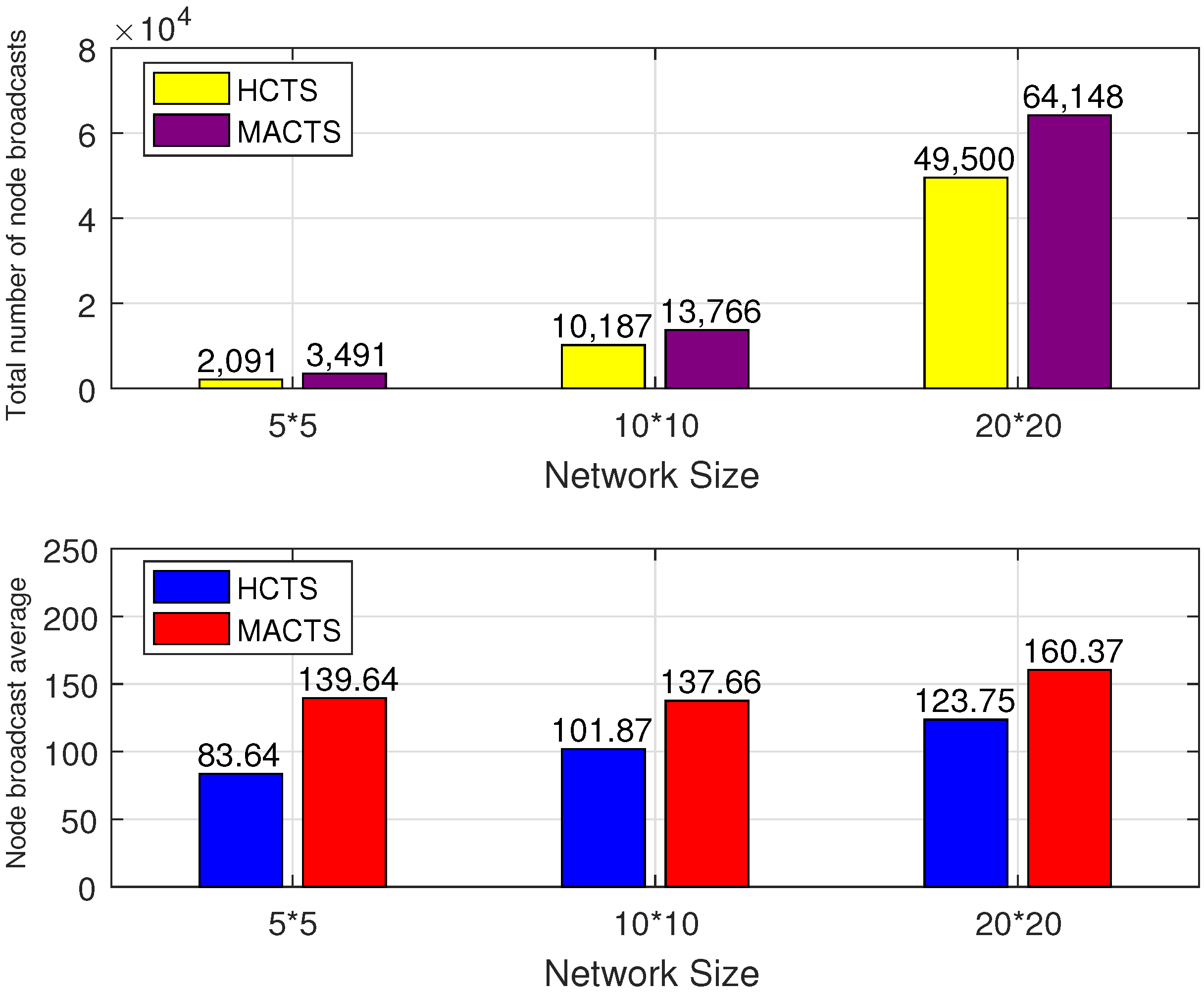
Since the HCTS algorithm is capable of rapidly achieving convergence and subsequently maintaining a low hop count for information transmission, it was observed that the number of broadcasts and the volume of transmitted information could be significantly reduced compared to other algorithms. Multiple simulations were performed under varying network scales while keeping other parameters constant, and the number of broadcasts required for nodes to achieve error convergence was recorded, as illustrated in Figure 8.

As shown in Figure 8, the number of broadcasts required for node convergence using the HCTS algorithm was lower than that required by the MACTS algorithm. For example, in a 20 × 20 grid network, the MACTS algorithm required a total of 64,148 broadcasts to achieve global error convergence, corresponding to an average of 160.37 broadcasts per node, whereas the proposed algorithm required only 49,500 broadcasts in total, with an average of 123.75 broadcasts per node.

5. Discussion

In this paper, we propose a hop-control time synchronization algorithm (HCTS) based on error convergence probability estimation, along with a corresponding adaptive hop-control mechanism. Both HCTS and MACTS are average-consensus-based algorithms and fully distributed time synchronization algorithms like ATS. These algorithms exhibit superior synchronization performance in dynamic networks with node mobility, packet loss, and topology changes, compared to centralized synchronization approaches. Moreover, they offer better scalability, making them well-suited for large-scale or evolving network environments.

5.1. Communication Cost

In WSNs, the energy expended by a node for transmission and reception operations constitutes the vast majority of its energy budget, whereas the sensor and processor consume comparatively little. Transmitting 1 bit of information over a distance of 100 m requires approximately the same energy as executing 3000 instructions. Consequently, reducing the total amount of information transmitted during a node’s lifetime directly lowers communication overhead. The total information transmitted is determined both by the length of individual data packets and by the total number of packets exchanged.

In this work, HCTS employs data packets of the same length as those used in MACTS and ATS—each packet carries only the node’s timestamp information—so variations in communication cost arise solely from differences in packet count. As shown in Figure 8, when network size increases, the number of packets required by HCTS to reach convergence is lower than that required by MACTS. Once synchronization has converged, the message complexity of HCTS is identical to that of both ATS and MACTS, since all three operate in a single-hop fashion. Moreover, during the synchronization setup phase, fewer message transmissions are incurred by HCTS than by ATS and MACTS. Therefore, to achieve faster convergence, it is cost-effective to introduce an appropriate increase in control complexity within HCTS.

5.2. Computational Cost

The synchronization models of HCTS, MACTS, and ATS are identical: one-way broadcasting is employed to exchange timestamps among nodes, after which clock parameters are estimated, and clock counter units are compared to achieve synchronization [24]. All three algorithms compute relative clock offset and relative clock rate using simple arithmetic operations, so their computational procedures—and hence their computational costs—are equivalent. Relative to ATS, HCTS and MACTS incur a slight increase in computational overhead due to the incorporation of multi-hop-control logic (basic arithmetic and logical operations). In particular, HCTS requires approximately 20 additional arithmetic or logical operations compared to MACTS. Thus, HCTS is characterized by its ease of implementation and its low energy overhead.

5.3. Limitations

If the parameters a, $L_p$, $\lambda$, and $\xi$ set either too small or too large, oscillatory behavior may occur in the multi-hop-control system under conditions of unstable time synchronization. Furthermore, HCTS is better suited to mesh topologies than to line topologies. Since HCTS relies on an average-consensus synchronization paradigm, its convergence speed and precision improve as the network’s algebraic connectivity increases [24]. Given the same number of nodes, a line network exhibits substantially lower algebraic connectivity than a mesh network. Accordingly, average-consensus methods are more appropriate for networks with many nodes arranged in a mesh topology.

6. Conclusions

The proposed HCTS is an improved version of the MACTS algorithm, where the original static multi-hop-control strategy in MACTS is enhanced with adaptive capabilities. Compared to MACTS, HCTS achieves faster convergence and higher synchronization accuracy. Additionally, HCTS significantly reduces communication overhead. Although it incurs slightly higher computational complexity than MACTS, the additional energy consumed by computation is negligible relative to the energy cost of wireless transmission. Therefore, HCTS offers improved overall energy efficiency. The hop count for each node is dynamically adjusted according to the real-time estimated convergence probability and the error variation rate of the synchronization process. This enables rapid error convergence during the initialization phase, improved accuracy during the maintenance phase, and reduced transmission overhead.

Experimental results demonstrate that the proposed algorithm significantly enhances synchronization precision, convergence speed, and communication efficiency. Notably, HCTS’s fine-grained timing alignment makes it highly suitable for microgrid applications, facilitating accurate state estimation, fault detection, and efficient renewable energy integration in distributed PMU networks.