Stock Price Prediction Using Candlestick Patterns and Sparrow Search Algorithm

Abstract

Accurately forecasting the trajectory of stock prices holds crucial significance for investors in mitigating investment risks and making informed decisions. Candlestick charts visually depict price information and the trends in stocks, harboring valuable insights for predicting stock price movements. Therefore, the challenge lies in efficiently harnessing candlestick patterns to forecast stock prices. Furthermore, the selection of hyperparameters in network models has a profound impact on the forecasting outcomes. Building upon this foundation, we propose a stock price prediction model SSA-CPBiGRU that integrates candlestick patterns and a sparrow search algorithm (SSA). The incorporation of candlestick patterns endows the input data with structural characteristics and time series relationships. Moreover, the hyperparameters of the CPBiGRU model are optimized using an SSA. Subsequently, the optimized hyperparameters are employed within the network model to conduct predictions. We selected six stocks from different industries in the Chinese stock market for experimentation. The experimental results demonstrate that the model proposed in this paper can effectively enhance the prediction accuracy and has universal applicability. In comparison to the LSTM model, the proposed model produces an average of 31.13%, 24.92%, and 30.42% less test loss in terms of MAPE, RMSE and MAE, respectively. Moreover, it achieves an average improvement of 2.05% in $R^2$.

1. Introduction

The stock market embodies an intricate and dynamic system replete with features like non-linearity, non-stationarity, volatility, and significant noise. These attributes render the change process of time series data, such as stock prices, susceptible to the influence of multifaceted factors, thereby imparting a profound sense of uncertainty to the direction of these changes [1,2]. Forecasting the movements of stock prices with precision can provide investors with a greater level of confidence in making informed decisions, leading to substantial gains. Consequently, the prediction of stock prices has emerged as a focal point of research within the realm of the financial market.

Experts and scholars have conducted extensive research on forecasting financial time series such as stock prices. The commonly used methods of technical analysis can be roughly categorized into three types: statistical analysis methods, machine-learning methods, and deep learning methods. Statistical analysis methods such as Autoregressive Moving Average (ARMA) [3], Autoregressive Integrated Moving Average (ARIMA), Generalized Autoregressive Conditional Heteroskedasticity (GARCH), and Autoregressive Conditional Heteroskedasticity (ARCH), have been extensively researched and applied by numerous scholars and investors. Jarrett et al. [4] used the ARIMA model to forecast and analyze the Chinese stock market. Juan et al. [5] applied the GARCH model to determine the predictive ability of Dubai International Airport’s activity volume on the UAE stock market. Given the inherent nonlinearity and excessive noise found in stock price data, the limitations arise when employing statistical analysis methods that assume a linear model structure. Consequently, achieving improved accuracy in predictions becomes challenging.

Machine-learning methods, such as Random Forest and Support Vector Machine (SVM), have been employed in the prediction of stock prices. This choice is motivated by their adeptness in capturing intricate relationships in time series data while simultaneously ensuring efficient computational performance. Lin et al. [6] utilized Principal Component Analysis to analyze and predict stocks, which provides a deeper exploration of machine-learning algorithms in the prediction field of financial time series data. Patel et al. [7] employed the naive Bayesian method for stock index prediction. Nti et al. [8] utilized the Random Forest method, optimized through decision tree optimization, to predict stock market indices and compared its performance against various traditional machine-learning models. Fu et al. [9] employed an SVM algorithm to predict financial time series data, yielding favorable prediction outcomes. Xu et al. [10] used an optimized integrated learning classifier to predict stock prices, thereby reducing prediction errors. The prowess of machine-learning techniques in the acquisition and processing of information from data falls short, despite notable strides in enhancing both speed and accuracy in predictions.

Deep learning, with its capacity for large-scale data processing, computation, and remarkable non-linear fitting ability, enables predictive models to deeply comprehend the profound correlation within the data. Common methods encompass the Back Propagation (BP) neural network, Recurrent Neural Network (RNN), Long Short-Term Memory (LSTM), Gated Recurrent Unit (GRU), etc. Zhang [11] contrasted the deep learning neural network model with the time series model, demonstrating that the neural network model is more capable of processing nonlinear data. Additionally, it outperformed the time series ARIMA model. Yu et al. [12] used the local linear embedding dimensional reduction algorithm (LLE) to diminish the dimensionality of factors influencing stock prices. Subsequently, they employed the BP neural network to forecast stock prices, thereby enhancing the accuracy of predictions. The employment of deep learning in the prediction framework has proven advantageous in accomplishing more accurate data predictions. Nonetheless, current prediction approaches and models necessitate further refinement. For instance, the information source exhibits a relatively narrow focus, primarily consisting of prevalent technical data, such as opening price, highest price, and lowest price, lacking comprehensive integration of other relevant information. Furthermore, the determination of hyperparameter magnitudes in models is typically reliant on experiential judgment, resulting in a challenging and rather subjective selection process.

Candlesticks are essentially daily samples of high-frequency price data, which can effectively express trend signals and have structural characteristics. In the empirical analysis, astute investors frequently anticipate fluctuations in stock prices by analyzing the candlestick series, confirming the inherent association between candlesticks and stock movements. Candlestick patterns are particular sequences of candlesticks on a candlestick chart that are primarily employed to identify trends. The candlestick pattern captures this information and portrays it in the form of a single candlestick or a combination of candlesticks with varying lengths [13].

However, employing candlestick patterns for the prediction of stock prices continues to be a challenging task. By learning and combing the existing research methods, this paper proposes a Bidirectional Gated Recurrent Unit Model Integrating Candlestick Patterns and a Sparrow Search Algorithm (SSA-CPBiGRU) model for stock price forecasting. The innovations and contributions of our work comprise the following three points:

• Currently, the primary information utilized for predicting stock prices is basic market data, which lacks structural relationships and exhibits limited expression capacity for the overall system state. This model ingeniously integrates candlestick patterns with stock market data, serving as input for the stock price prediction model, imbuing the input data with structural characteristics and time series relationships. Furthermore, this paper uses a Bidirectional Gated Recurrent Unit (BiGRU) network to extract deeper feature relationships, thereby enhancing the learning ability of the network;
• This paper applies a sparrow search algorithm (SSA) [14] to stock price forecasting, addressing the challenge of high randomness and difficulty in hyperparameter selection of the CPBiGRU network. Simultaneously, it enhances the accuracy of stock price forecasting;
• Current research typically utilizes data from the same time window for forecasting. However, in actual trading decisions, investors often refer to stock price information from multiple trading days. Therefore, this paper explores the impact of extracting stock data from different time windows on prediction results.

The rest of the paper is organized as follows. Related work is covered in Section 2. The methodology is explained in Section 3. Section 4 presents the results, showing the experiments performed, and Section 5 provides the conclusions, with future directions listed in detail.

2. Related Work

We discuss published literature in two different categories here. These categories are related to candlestick patterns analysis and using deep learning models in stock prediction, respectively. The models pertaining to these domains is reviewed in detail and elaborated on.

2.1. Candlestick Patterns Analysis

Candlestick charts are a form of technical analysis visualization that are created by plotting the opening, highest, lowest, and closing prices of each analysis period [15]. Figure 1 represents an example of a candlestick chart. A box used to represent the difference between the open price and the close price is called the body of the candlestick. When the close price is higher than the open price, the body color is red, otherwise the body is green. The research environment of candlestick patterns is multifaceted. It can be categorized into three primary cases: sequential pattern mining and its applications, candlesticks and their applications, and stock time series forecasting.

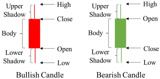
Figure 1. Example of candlestick chart.

The sequential pattern mining algorithms have mainly concentrated on discovering rules, generating sequences, combining resources [16], and predicting sequences. Aiming for accurate destination forecasting, and giving its first partial trip trajectory as input, Iqbal et al. [17] considered it a multi-class prediction problem and proposed an efficient, non-redundant contrast sequence miner algorithm to distinguish mine patterns, which can only be seen in one class. Li et al. [18] proposed a one-pass algorithm, with a commonly used frequency as the output for a given sequence, and two advanced models to further improve the processing efficiency of voluminous sequences and streaming data. To address the shortcomings of traditional sequence pattern mining algorithms, Wang et al. [19] proposed a timeliness variable threshold and an increment Prefixspan algorithm, verifying the effectiveness of the algorithm. Sophisticated investors can analyze candlestick sequences in historical data and speculate on the patterns that will appear in the next period, thus enabling them to prognosticate future trends in stock markets. Candlesticks and their applications mainly focus on the image processing of candlesticks, identifying and interpreting certain candlestick patterns, while also striving to enhance recognition accuracy. Birogul et al. [20] and Guo et al. [21] encoded candlestick data into 2D candlestick charts and learned the morphological features of the candlestick data through deep neural networks. Chen et al. [22] proposed a two-step approach for the automatic recognition of eight candlestick patterns, with an average accuracy surpassing that of the LSTM model. Fengqian et al. [23] used candlestick charts as a generalization of price data across a timeframe, serving as a denoising tool. They subsequently employed cluster analyses and reinforcement learning methods to achieve online adaptive control of parameters within unfamiliar environments, ultimately enabling the implementation of high frequency transaction strategies.

Stock time series forecasting is mainly divided into two categories: stock price forecasting and stock trend forecasting. Wang et al. [24] evaluated the effectiveness of several renowned candlestick patterns, employing recent data from 20 American stocks to estimate stock prices. Udagawa et al. [13] proposed a hybrid algorithm that combines candlesticks sharing a specific price range into a single candlestick, thereby eliminating noisy candlesticks. Madbouly et al. [25] combined a cloud model, fuzzy time series and Heikin-Ashi candlesticks to forecast stock trends, thereby enhancing the accuracy of predictions. Wang et al. [26] proposed a quantification method for stock market candlestick charts based on the Hough variation. They utilized the graph structure embedding method and multiple attention graph neural networks to improve the prediction performance of stock prices.

2.2. Deeping Learning Approaches in Stock Prediction

Currently, deep learning approaches have become the predominant focus of research both domestically and internationally. Numerous experts and scholars have dedicated their efforts to exploring this field extensively. Rather et al. [27] used RNN with memory capability to predict stock returns. Minami [28] employed a variant RNN model called LSTM, which effectively alleviates common issues in neural networks such as gradient vanishing and explosions, as well as long-range dependence. Gupta et al. [29] augmented prediction speed by adopting GRU, a network structure with fewer gating mechanisms compared to LSTM, as the main network structure of the prediction model. Chandar et al. [30] used s wavelet neural network model to predict stock price trends. The aforementioned scholars have utilized historical stock price data at the input level of their models in order to conduct their prediction research. Additionally, deep learning techniques for stock prediction can incorporate a wider and more varied range of information sources, thereby enriching the factors influencing the prediction model. Cai et al. [31] integrated the characteristics of financial- and stock market-related news posts into a hybrid model consisting of a LSTM and Convolutional Neural Network (CNN) for forecasting. They constructed the prediction model using a multi-layer recurrent neural network. However, although the complexity of the model was increased, the prediction accuracy could be further improved. Ho et al. [32] combined candlestick charts with social media data, proposing a multi-channel collaborative network for predicting stock trends.

Furthermore, the current existing network models still have certain limitations. The selection of hyperparameters in these models is often based on existing research or experience, coming with a certain degree of subjectivity. Appropriate hyperparameters can improve the topology of the network model and enhance its generalization and fitting capabilities. Hence, the issue of eliminating the influence of human factors and finding the optimal network model hyperparameters is a matter of concern for scholars. Hu [33] employed a Bayesian algorithm to optimize the learning rate, the number of hidden layers, and the number of neurons within LSTM, with the goal of forecasting the stock prices of prominent stocks at specific stages of the Chinese stock market. The experimental results demonstrated that the optimized model possesses high universality and efficacy. Optimization of important parameters in the proposed network by a swarm intelligent optimization algorithm can solve the problems of network hyperparameters selection with high randomness, difficult selection, and influence by human factors, improving the prediction accuracy [34,35]. Song et al. [36] utilized the Particle Swarm Optimization (PSO) with adaptive learning strategy to optimize the time step, the batch size, the number of iterations, and the number of hidden layer neurons in the LSTM network. The SSA has a stronger optimization ability than the Grey Wolf Optimization (GWO), Ant Colony Optimization (ACO), and PSO [14]. Li et al. [37] conducted a comprehensive investigation comparing the Bat Algorithm (BA), GWO, Dragonfly Algorithm (DA), Whale Optimization Algorithm (WOA), Grasshopper Optimization Algorithm (GOA), and SSA. The performance of these algorithms, including their convergence speed, accuracy, and stability, was compared using 22 standard CEC test functions. The results clearly demonstrated that the SSA surpassed the other five algorithms in all aspects. Liao [38] utilized the SSA to optimize the weights, bias, the number of neurons in the hidden layer, and the number of iterations within the LSTM network. This methodology has heightened the prediction accuracy of the model and has been effectively implemented to address load forecasting issues with favorable results.

3. Methodology

The full system diagram is shown in Figure 2. Firstly, the stock market data and candlestick are preprocessed separately. Subsequently, the CPBiGRU optimized by SSA is utilized to forecast the closing price of stocks. Finally, the evaluation metrics are employed to evaluate the model performance.

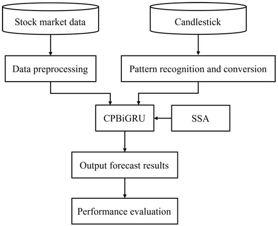
Figure 2. System diagram of the proposed method.

3.1. BiGRU Network

The GRU model proposed by Cho et al. [39] is a variant of LSTM. GRU simplifies the input gate and forget gate in LSTM into an update gate, which controls the input and previous output to be transferred to the next cell. Additionally, it sets a reset gate to regulate the amount of historical information to be forgotten. It can effectively avoid the problems of long-range dependence and insufficient memory capacity of traditional recurrent neural networks. In contrast to LSTM, GRU exhibits a more simple architecture, as well as faster training and fitting speeds [40]. The architecture of the GRU is shown in Figure 3, and the operation formula is defined by Equations (1)–(4).

$$z_t=\sigma (W_z·\left[h_{t-1},x_t\right]+b_z)$$

(1)

$$r_t=\sigma (W_r·[h_{t-1},x_t]+b_r)$$

(2)

$$\widetilde{h_t}=tanh(W·[{r_t\ast h}_{t-1},x_t]+b_{\tilde{h}})$$

(3)

$$h_t=\left(1-z_t\right)\ast h_{t-1}+z_t\ast \widetilde{h_t}$$

(4)

where $x_t$ and $h_t$ represent the input value and output value of the GRU network at moment $t$, respectively. In addition, $h_{t-1}$ is the output at the previous moment, $\widetilde{h_t}$ is the candidate value of the memory cell value at moment $t$, $r_t$ represents the reset gate, and $z_t$ represents the update gate. $W_z$, $W_r$, and $W$ are the weight matrices of the update gate, reset gate and candidate hidden layer state, respectively. $b_z,b_r$, and $b_{\tilde{h}}$ are the bias terms of the update gate, reset gate and candidate hidden layer state, respectively, while $\sigma$ is the sigmoid activation function.

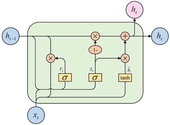
Figure 3. GRU architecture block diagram.

However, the GRU network only considers unidirectional information flow while disregarding the influence of other directions of information flow. The lack of sufficient influential factors and information characteristics for data at prediction points imposes certain limitations on the predictive performance of the network. BiGRU is a neural network architecture that considers information flow in both historical and future directions. Building upon the foundation of the unidirectional GRU, it incorporates an additional layer of reverse-GRU. It not only improves the issue of temporal dependencies in data, but also expands the number of neural units, enabling more precise prediction results. Therefore, we choose BiGRU as the foundational model for prediction methodology.

The output value of BiGRU network unit is obtained by combining the hidden unit output values in both backward and forward directions. The final output of BiGRU is calculated as shown in Equation (5): where $w_t$ and $v_t$ represent the weights corresponding to the forward hidden layer state $\overrightarrow{h_t}$ and the reverse hidden layer state $\overleftarrow{h_t}$ corresponding to the BiGRU at moment $t$, $b_t$ represents the offset corresponding to the hidden layer state at moment $t$. The structure diagram of BiGRU is shown in Figure 4.

$$h_t=w_t\overrightarrow{h_t}+v_t\overleftarrow{h_t}+b_t$$

(5)

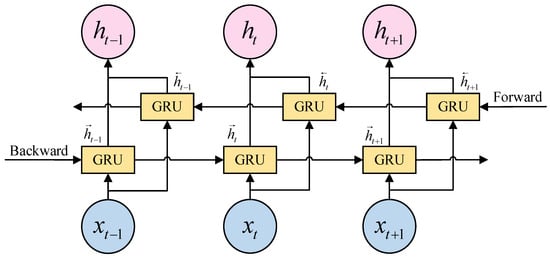
Figure 4. BiGRU structure diagram.

3.2. A Dual Port BiGRU Network Integrating Candlestick Patterns

Candlestick patterns reflect the market trend and price information, and they can be roughly divided into two categories: reversal patterns and continuation patterns. Talib is a Python quantitative indicator library, offering functions to identify 61 candlestick patterns. These functions return three values: 0, 100 and −100. Here, 100 indicates recognition of the pattern, while −100 indicates recognition of the pattern’s inverse form, 0 indicates that the candlestick pattern is not recognized, 100 indicates the recognition of the pattern, and −100 indicates the recognition of the pattern’s inverse form. Since the return values of different patterns indicate different market trends, they cannot be directly incorporated into the stock price prediction models. The experiment defines three kinds of stock trend prediction values: −1, 0, and 1. Here, −1 indicates a downward trend in the stock, 1 indicates an upward trend in the stock, and 0 indicates that the candlestick pattern is not detected. In this paper, the return values of 61 candlestick patterns are transformed into corresponding stock trend prediction values based on the pattern definition. The generated correlation table of stock trend prediction values is presented in Table 1. For example, the candlestick pattern of two crows predicts a falling stock price. When this pattern is identified, the function in Talib that recognizes this pattern will return a value of 100. When the reverse pattern is identified, the function will return a value of −100. Therefore, in the correlation table of stock trend predictions, the return values of 100 and −100 for the two crows pattern correspond to stock trend predictions of −1 and 1, respectively.

Table 1. The correlation table of stock trend prediction values.

Candlestick Patterns	Return Value	Predictive Trending	Candlestick Patterns	Return Value	Predictive Trending
Two Crows	100	−1	Identical Three Crows	100	−1
	−100	1		−100	−1
Three Black Crows	100	−1	In-Neck Pattern	100	1
	−100	1		−100	−1
Three Inside Up/Down	100	1	Inverted Hammer	100	1
	−100	−1		−100	−1
Three Line Strike	100	1	Kicking	100	1
	−100	−1		−100	−1
Three Outside Up/Down	100	1	Kicking-bull/bear determined by the longer marubozu	100	1
	−100	−1		−100	−1
Three Stars In The South	100	1	Ladder Bottom	100	1
	−100	−1		−100	−1
Three Advancing White Soldiers	100	1	Long Legged Doji	100	1
	−100	−1		−100	−1
Abandoned Baby	100	1	Long Line Candle	100	1
	−100	−1		−100	−1
Advance Block	100	1	Marubozu	100	1
	−100	−1		−100	−1
Belt-hold	100	1	Matching Low	100	1
	−100	−1		−100	−1
Breakaway	100	1	Mat Hold	100	1
	−100	−1		−100	−1
Closing Marubozu	100	1	Morning Doji Star	100	1
	−100	−1		−100	−1
Concealing Baby Swallow	100	1	Morning Star	100	1
	−100	−1		−100	−1
Counterattack	100	1	On-Neck Pattern	100	1
	−100	−1		−100	−1
Dark Cloud Cover	100	−1	Piercing Pattern	100	1
	−100	1		−100	−1
Doji	100	1	Rickshaw Man	100	1
	−100	−1		−100	−1
Doji Star	100	1	Rising/Falling Three Methods	100	1
	−100	−1		−100	−1
Dragonfly Doji	100	1	Separating Lines	100	1
	−100	−1		−100	−1
Engulfing Pattern	100	1	Shooting Star	100	−1
	−100	−1		−100	1
Evening Doji Star	100	1	Short Line Candle	100	1
	−100	−1		−100	−1
Evening Star	100	1	Spinning Top	100	−1
	−100	−1		−100	1
Up/Down-gap side-by-side white lines	100	1	Stalled Pattern	100	1
	−100	−1		−100	−1
Gravestone Doji	100	1	Stick Sandwich	100	1
	−100	−1		−100	−1
Hammer	100	1	Takuri	100	−1
	−100	−1		−100	1
Hanging Man	100	1	Tasuki Gap	100	1
	−100	−1		−100	−1
Harami Pattern	100	1	Thrusting Pattern	100	1
	−100	−1		−100	−1
Harami Cross Pattern	100	1	Tristar Pattern	100	1
	−100	−1		−100	−1
High-Wave Candle	100	−1	Unique 3 River	100	1
	−100	1		−100	−1
Hikkake Pattern	100	1	Upside Gap Two Crows	100	−1
	−100	−1		−100	1
Modified Hikkake Pattern	100	1	Upside/Downside Gap Three Methods	100	1
	−100	−1		−100	−1
Homing Pigeon	100	1
	−100	−1

If multiple candlestick patterns are recognized on a certain day, the stock trend prediction for that day is the sum of the corresponding stock trend predictions for all identified patterns, e.g, if the engulfing pattern and belt-hold pattern are detected on a certain day, and the return values for both patterns are 100. Firstly, we refer to the correlation table to find the corresponding stock trend prediction value of 1 for these two patterns. Then, we add the trend prediction values for these two patterns together, resulting in a stock trend prediction value of 2 for this day. The stock trend prediction value and the stock market data are individually normalized and employed as inputs to the CPBiGRU network. The flowchart of CPBiGRU model is shown in Figure 5.

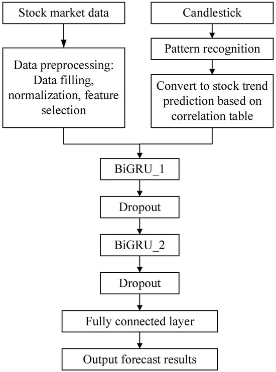
Figure 5. Flowchart for CPBiGRU.

3.3. Principle of Sparrow Search Algorithm

SSA is a novel swarm intelligence optimization technique. The algorithm simulates the foraging behavior of sparrow populations, dividing the sparrow population into discoverers and joiners. SSA calculates the fitness value of sparrows through the constructed fitness function, thus achieving the role and position transformation between individual sparrows, effectively avoiding the issue of traditional optimization algorithms easily getting stuck in local optima.

The population composed of n sparrows can be expressed as follows: where $X$ is a randomly initialized sparrow population, $x$ is an individual sparrow, $d$ represents the dimensionality of the population, and $n$ is the number of sparrows.

$$X=\left[\begin{array}{cc}\begin{array}{cc}{x}_{1,1}& x_{1,2}\\ x_{2,1}& x_{2,2}\end{array}& \begin{array}{cc}\dots & x_{1,d}\\ \dots & x_{2,d}\end{array}\\ \begin{array}{cc}⋮& ⋮\\ x_{n,1}& x_{n,2}\end{array}& \begin{array}{cc}⋮& ⋮\\ \dots & x_{n,d}\end{array}\end{array}\right]$$

(6)

The fitness values of all sparrows can be expressed as follows: where $F_x$ is the fitness matrix, $f$ is the fitness value, expressed as the Root Mean Squared Error (RMSE) between the stock price prediction data and the real price data.

$$F_x=\left[\begin{array}{c}f\left(\left[x_{1,1}{x}_{1,2}\dots x_{1,d}\right]\right)\\ f\left(\left[x_{2,1}{x}_{2,2}\dots x_{2,d}\right]\right)\\ \begin{array}{c}⋮\\ ⋮\\ f\left(\left[x_{n,1}{x}_{n,2}\dots x_{n,d}\right]\right)\end{array}\end{array}\right]$$

(7)

The discoverers search for food and provide foraging direction to all joiners. During each iteration, the formula for the discoverer update location can be described using the following equation: where $t$ is the current iteration number, $j=1,2,3,\dots ,d$, ${iter}_{max}$ is the maximum number of iterations and is a constant, $X_{i,j}$ represents the position information of the $i$-th sparrow in the $j$-th dimension, $\alpha$ is a random number in [0, 1]. $Q$ is a random number that follows a normal distribution, and $L$ is a $1\times d$ matrix in which each element is 1. $R_2(R_2\in [0,1\left]\right)$ and $ST(ST\in [0.5,1.0\left]\right)$ are the alarm value and the safe value, respectively. When $R_2<ST$, it indicates the absence of predators in the environment, allowing the discoverers to conduct extensive searches. When $R_2\ge ST$, it indicates that certain individuals within the population have detected predators and they will immediately emit an alarm signal. Following the reception of these alarm signals, the population is required to move to a secure location.

$$X_{i,j}^{t+1}=\left\{\begin{array}{cc}{X}_{i,j}^t·\exp \left(\frac{-i}{\alpha ·{iter}_{max}}\right)& R_2<ST\\ X_{i,j}^t+Q·L& R_2\ge ST\end{array}\right.$$

(8)

During the foraging process, joiners continuously revise their positions in order to acquire food while simultaneously keeping an eye on discovers and competing with them for food. Equation (9) outlines the approach used by joiners to update their positions. When $i>n/2$, it indicates that the $i$-th joiner with a lower fitness value has not obtained food and needs to fly to other places to search for more. Where $X_P$ represents the location of the optimal discoverer, $X_{worst}$ represents the current global worst position, $n$ is the population size, while A is a $1\times d$ matrix where each element is randomly assigned as 1 or −1, and $A^{+}=A^T{\left(A{A}^T\right)}^{-1}$.

$$X_{i,j}^{t+1}=\left\{\begin{array}{cc}Q·\exp \left(\frac{X_{worst}^t-X_{i,j}^t}{i^2}\right)& i>\frac{n}{2}\\ X_P^{t+1}+\left|X_{i,j}^t-X_P^{t+1}\right|·A^{+}·L& i\le \frac{n}{2}\end{array}\right.$$

(9)

In the algorithm, it is assumed that between 10% and 20% of sparrows in the population will become aware of danger and emit alarm signals when the danger occurs. The initial positions of these sparrows are randomly generated in the population, and their positions are updated based on Equation (10). Where $X_{best}$ represents the current global optimal position, $\beta$ is a step size control parameter following a normal distribution with a mean of 0 and a variance of 1. $K$ is a random number in [−1, 1] that indicates the direction of sparrow movement and also serves as a step size control parameter. Additionally, $f_i$ represents the fitness value of the $i$-th sparrow individual, while $f_g$, $f_w$ represent the current global optimal and worst fitness values, respectively, and $\epsilon$ is an extremely small constant to avoid the error of zero division.

$$X_{i,j}^{t+1}=\left\{\begin{array}{cc}{X}_{best}^t+\beta ·\left|X_{i,j}^t-X_{best}^t\right|& f_i>f_g\\ X_{i,j}^t+K·\left(\frac{\left|X_{i,j}^t-X_{worst}^t\right|}{\left(f_i-f_w\right)+\epsilon }\right)& f_i=f_g\end{array}\right.$$

(10)

When $f_i>f_g$, it means that this sparrow is at the edge of the population and is extremely vulnerable to predators. When $f_i=f_g$, it indicates that the sparrow in the middle of the population perceives the danger and needs to approach the other sparrows in time in order to reduce the risk of predation.

The flowchart of the SSA-CPBiGRU model is shown in Figure 6. It can be divided into the following five steps:

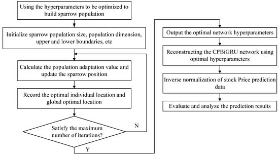
Figure 6. Flowchart for SSA-CPBiGRU.

• Initialization: We take the learning rate, iteration times and the number of units in two hidden layers of the CPBiGRU network as the hyperparameter objectives to be optimized by the SSA. The position information of the population and related parameters are randomly initialized after setting the value range of the optimized hyperparameter, the population size of sparrows, optimization iteration times, and initial safety threshold value;
• Fitness value: We use the RMSE between the predicted value of the network model and the real value as the fitness function for SSA and the loss function for CPBiGRU, to determine the fitness values of each sparrow;
• Update: We update the sparrow position by Equations (8)–(10) and obtain the fitness value of the sparrow population. Simultaneously, we record the optimal individual position and global optimal position value in the population;
• Iteration: We ascertain if the maximum value of the number of update iterations has been attained. In such a case, conclude the loop and yield the optimal individual solution, signifying the determination of the optimal parameters for the network structure. Otherwise, return to step (3);
• Optimization results output: The optimal hyperparameter values output by the SSA algorithm are employed as the learning rate, iteration number, and number of units in two hidden layers of the CPBiGRU network. Afterwards, the network is reconstructed and we proceed with subsequent procedures such as inverse normalization and evaluation analysis.

4. Experiments and Discussions

4.1. Experimental Environment

The operating system of the experimental equipment is Windows 11, the graphics card is Nvidia GeForce RTX 3060, the code is written in Python language, and the prediction model is simulated and experimented with in the Keras framework, which is integrated with Tensorflow 2.9. The learning rate, number of iterations, and number of units in two hidden layers of the CPBiGRU network are obtained by SSA optimization. The search ranges for the hyperparameters are as follows: the learning rate is defined between [0.001, 0.01], the search range for the number of iterations is set as [10, 100], and the number of units in the hidden layers is between [1, 100]. The settings for other hyperparameters are outlined in Table 2.

Table 2. Model hyperparameter settings.

Hyperparameter	Value
Batch size	128
Optimizer	Adam
Number of hidden layer units	2
SSA population size	10
SSA iterations	20
SSA discoverer ratio	0.2

4.2. Datasets

The dataset used in this article consists of two parts: stock market data and stock trend prediction value, both collected on a daily basis, with a time span from 1 January 2017 to 1 August 2022.

To ensure the accuracy of the experimental data source, the stock market data are downloaded from the BaoStock data interface package in Python. In order to verify the universality and effectiveness of the model, this experiment selected six representative stocks from different sectors and industries as the research objects, as shown in Table 3.

Table 3. Stock dataset statistics.

Stock	Plate	Sector
SH.600000	Main Board of the Shanghai Stock Exchange	Bank
SH.603589	Main Board of the Shanghai Stock Exchange	Liquor
SH.600104	Main Board of the Shanghai Stock Exchange	Automobile
SZ.300294	Shenzhen Stock Exchange GEM	Medicine
SZ.002415	Shenzhen Stock Exchange SME	Computer
SZ.000725	Main Board of the Shenzhen Stock Exchange	Electron

The Pearson correlation coefficient is a method used to measure the correlation between two variables, and its values are in the range of [−1, 1] [41]. The formula is represented as Equation (11). Where ${\rho }_{X,Y}$ is the correlation coefficient, ${\sigma }_X$ and ${\sigma }_Y$ are the standard covariance of variables $X$ and $Y$, respectively. Additionally, $cov\left(X,Y\right)$ is the covariance between $X$ and $Y$, and ${\mu }_X$ and ${\mu }_Y$ represent the means of $X$ and $Y$, respectively. When ${\rho }_{X,Y}>0$, it indicates a positive correlation between $X$ and $Y$. When ${\rho }_{X,Y}<0$, it indicates a negative correlation between $X$ and $Y$. By computing the Pearson correlation coefficients between various market data, a heatmap of the stock market data, as shown in Figure 7, can be generated. From the heatmap, it is evident that the price-to-cashflow ratio (pcfNcfTTM) is negatively correlated with the closing price (close). The objective of this experiment is to predict the closing price of an individual stock. Therefore, we selected 11 kinds of stock market data, including open, high, low, close, pctChg, volume, turn, amount, psTTM, peTTM, and pbMRQ.

$${\rho }_{X,Y}=\frac{cov(X,Y)}{{\sigma }_X{\sigma }_Y}=\frac{E\left[(X-{\mu }_X)(Y-{\mu }_Y)\right]}{{\sigma }_X{\sigma }_Y}$$

(11)

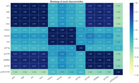
Figure 7. A heatmap of stock market data.

At the same time, the daily trend prediction value of the target stock is obtained based on the correlation table of stock trend prediction values. The stock market data and the trend prediction value are synchronized based on trading time, serving as input data to train SSA-CPBiGRU network for forecasting the closing price of stocks on the following day. The dataset comprises a total of 1356 days, arranged in chronological order. The top 65%, 10%, and the remaining 25% of the dataset are respectively allocated as the training set, validation set, and test set.

4.3. Data Preprocessing

4.3.1. Missing Value Processing

The obtained stock data may have the problem of missing data and suspension of trading, and these missing data may have an impact on stock price prediction. We employ the mean-filling method to fill in missing data. For the data on the suspension date, we adopt the data from the day before the suspension date for filling, thereby ensuring the integrity of the data.

4.3.2. Data Standardization

Due to the large magnitude of stock data and the different magnitudes of input features, directly inputting them into the network model will lead the model bias towards features with large magnitudes, resulting in features with smaller magnitudes not being effective. Therefore, in order to eliminate the effect of different magnitudes between features, the paper uses the maximum minimum standardization method to normalize the stock data to the range of [0, 1]. The formula is as follows:

$${y_i}^{’}=\frac{y_i-y_{min}}{y_{max}-y_{min}}$$

(12)

where $y_i$ is the denoised stock data, ${y_i}^{’}$ is the normalized data as the input value of the model, $y_{max}$ and $y_{min}$ are the maximum and minimum values in the data, respectively.

$$y=y^{\ast }\left(y_{max}-y_{min}\right)+y_{min}$$

(13)

where $y$ is the predicted value of the inverse normalization of the model, $y^{\ast }$ is the predicted value of the model, $y_{min}$ is the minimum value of the original data in the test set, and $y_{max}$ is the maximum value of the original data in the test set.

4.4. Evaluation Criteria

In order to show the prediction effect of each model, we evaluate the performance of each model by using four metrics: Mean Absolute Percentage Error (MAPE), RMSE, Mean Absolute Error (MAE), and Coefficient of Determination ($R^2$). The smaller the values of MAPE, RMSE and MAE, the higher the accuracy of the prediction model and the better the prediction effect. As the value of $R^2$ approaches closer to one, the model’s fitting performance grows increasingly superior. The formulas for the four indicators are defined by Equations (14)–(17). Where $y_i$ is the true value of stock closing price, ${y_i}^{’}$ is the predicted value of stock closing price, $\overline{y}$ is the average value of the true value of the sample, and $n$ is the sample size of the test dataset.

$$MAPE=\frac{100\%}{n}\sum _{i=1}^n\left|\frac{y_i-{y_i}^{’}}{y_i}\right|$$

(14)

$$RMSE=\sqrt{\frac{1}{n}\sum _{i=1}^n{(y_i-{y_i}^{’})}^2}$$

(15)

$$MAE=\frac{1}{n}\sum _{i=1}^n\left|y_i-{y_i}^{’}\right|$$

(16)

$$R^2=1-\frac{\sum _i{\left({{y_i}^{’}-y}_i\right)}^2}{\sum _i{\left({\overline{y}-y}_i\right)}^2}$$

(17)

4.5. Comparing the Prediction Accuracy

4.5.1. Experimentation and Analysis of Stock Price Prediction Model

In order to better evaluate the performance of the models and examine the effectiveness of incorporating candlestick patterns into stock price prediction, LSTM, GRU, BiGRU, CPBiGRU, SSA-BiGRU and SSA-CPBiGRU models are selected for comparative experiments in this paper. To mitigate the element of chance in the experiments and ensure the reliability of the experimental results, we conducted five experiments for each model to obtain the average value. The specific experimental results are shown in Table 4, where the bolded data represent the best predicted experimental results. The prediction results of each model on all stock data test sets selected for the experiment are shown in Figure 8, Figure 9, Figure 10, Figure 11, Figure 12 and Figure 13.

Table 4. Predictive performance of different models.

Model	Stock	MAPE	RMSE	MAE	${\mathit{R}}^2$
LSTM	SH.600000	0.0137	0.1489	0.1178	0.9756
	SH.603589	0.0277	2.3260	1.7570	0.9264
	SH.600104	0.0168	0.4178	0.3157	0.9392
	SZ.300294	0.0337	1.6722	1.2259	0.9088
	SZ.002415	0.0311	2.1352	1.6488	0.9538
	SZ.000725	0.0332	0.1845	0.1650	0.9649
GRU	SH.600000	0.0120	0.1313	0.1080	0.9810
	SH.603589	0.0262	2.2027	1.6451	0.9340
	SH.600104	0.0142	0.3813	0.2714	0.9493
	SZ.300294	0.0325	1.6306	1.1828	0.9132
	SZ.002415	0.0295	2.0208	1.5643	0.9585
	SZ.000725	0.0316	0.1802	0.1594	0.9665
BiGRU	SH.600000	0.0102	0.1152	0.0906	0.9854
	SH.603589	0.0249	2.1920	1.5678	0.9347
	SH.600104	0.0139	0.3720	0.2688	0.9518
	SZ.300294	0.0319	1.6146	1.1758	0.9149
	SZ.002415	0.0232	1.5993	1.2063	0.9741
	SZ.000725	0.0235	0.1421	0.1205	0.9792
CPBiGRU	SH.600000	0.0094	0.1079	0.0834	0.9871
	SH.603589	0.0245	2.1829	1.5543	0.9352
	SH.600104	0.0137	0.3657	0.2641	0.9536
	SZ.300294	0.0304	1.6077	1.1262	0.9157
	SZ.002415	0.0216	1.4820	1.1078	0.9777
	SZ.000725	0.0191	0.1248	0.0990	0.9839
SSA-BiGRU	SH.600000	0.0086	0.1066	0.0768	0.9875
	SH.603589	0.0241	2.0366	1.4912	0.9433
	SH.600104	0.0136	0.3639	0.2619	0.9539
	SZ.300294	0.0293	1.4882	1.0839	0.9277
	SZ.002415	0.0209	1.4449	1.0710	0.9788
	SZ.000725	0.0177	0.1160	0.0918	0.9861
SSA-CPBiGRU	SH.600000	0.0077	0.0989	0.0689	0.9892
	SH.603589	0.0235	2.0330	1.4685	0.9439
	SH.600104	0.0134	0.3639	0.2601	0.9542
	SZ.300294	0.0282	1.4572	1.0290	0.9307
	SZ.002415	0.0193	1.3275	0.9654	0.9821
	SZ.000725	0.0155	0.1112	0.0834	0.9872

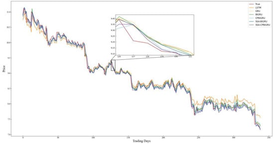
Figure 8. Comparison chart of SH.600000 prediction results.

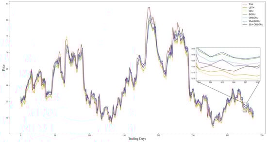
Figure 9. Comparison chart of SH.603589 prediction results.

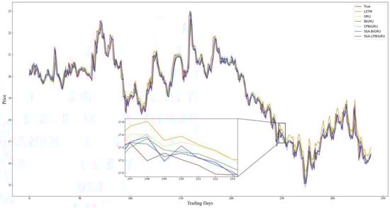
Figure 10. Comparison chart of SH.600104 prediction results.

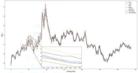
Figure 11. Comparison chart of SZ.300294 prediction results.

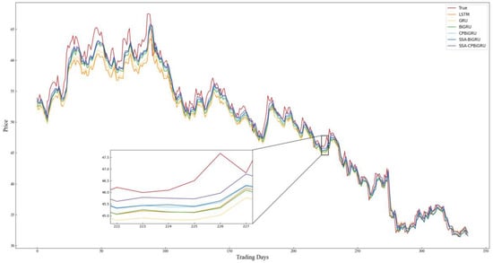
Figure 12. Comparison chart of SZ.002415 prediction results.

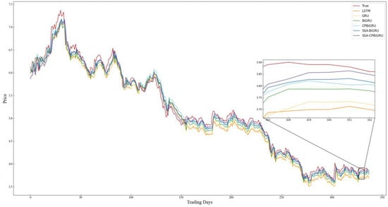
Figure 13. Comparison chart of SZ.000725 prediction results.

Combining the prediction results in Table 4 and Figure 8, Figure 9, Figure 10, Figure 11, Figure 12 and Figure 13, it can be seen that the SSA-CPBiGRU model has a better prediction performance than other models. From Table 4, it can be seen that the BiGRU model has better prediction results than LSTM and GRU. In comparison to the LSTM model, the BiGRU model reduces the test loss by an average reduction of 18.81%, 15.15%, and 17.77% in terms of MAPE, RMSE and MAE, respectively. Additionally, there is an average improvement of 1.24% in $R^2$. This is mainly due to the fact that BiGRU improves the problem of data time dependence and increases the number of neural units, which leads to more accurate prediction results.

Compared with the single LSTM, GRU and BiGRU models, the CPBiGRU model exhibits a significant improvement in terms of MAPE, RMSE, and MAE. In comparison to the BiGRU model, the CPBiGRU model produces an average of 6.87%, 4.73%, and 6.80% less test loss in terms of MAPE, RMSE and MAE, respectively. This indicates that the addition of candlestick patterns contributes to an enhancement in stock price forecasting performance.

In addition, SSA-BiGRU and SSA-CPBiGRU, which use SSA to optimize the hyperparameters of the model, outperform the model with manually defined hyperparameter values in all evaluation criteria. Compared to the CPBiGRU model, the SSA-CPBiGRU model reduces the test loss by an average reduction of 10.18%, 7.73%, and 10.28% in terms of MAPE, RMSE and MAE, respectively. This indicates that the utilization of SSA can help to improve the prediction accuracy of the model.

The SSA-CPBiGRU model proposed in this paper outperformed the previous five models in predicting the closing prices of stocks in six different sectors and industries. In comparison to the BiGRU model, the SSA-CPBiGRU model produces an average of 16.03%, 12.01%, and 16.13% less test loss in terms of MAPE, RMSE and MAE, respectively, and it also achieves an average improvement of 0.82% in $R^2$. Moreover, when compared to the GRU model, the SSA-CPBiGRU model reduces the test loss by an average reduction of 25.09%, 20.03%, and 25.01% in terms of MAPE, RMSE and MAE, respectively. Additionally, there is an average improvement of 1.46% in $R^2$. In comparison to LSTM model, the SSA-CPBiGRU model exhibits an average reduction of 31.13%, 24.92%, and 30.42% in test loss in terms of MAPE, RMSE, and MAE, respectively. Additionally, it achieves an average enhancement of 2.05% in $R^2$.

Based on the above analysis, the SSA-CPBiGRU model demonstrates superior efficacy in forecasting stock prices compared to traditional network models, exhibiting reduced prediction errors and enhanced fitting capabilities.

4.5.2. Experimentation and Analysis of the Effect of Trading Day on Stock Price Prediction

Based on the above experiments, we aim to determine how long the trading day of stock data can achieve the optimal stock price prediction effect. In Table 5, SSA-CPBiGRU (1), SSA-CPBiGRU (2), SSA-CPBiGRU (3), SSA-CPBiGRU (5), and SSA-CPBiGRU (10) represent the use of stock data from the first trading day, the first two trading days, the first three trading days, the first five trading days, and the first ten trading days of the predicted stock price date in the model for prediction. Bolded data in the table denote the experimental results of the optimal prediction.

Table 5. Predictive performance of different trading days.

Model	Stock	MAPE	RMSE	MAE	${\mathit{R}}^2$
SSA-CPBiGRU (1)	SH.600000	0.0095	0.1149	0.0835	0.9854
	SH.603589	0.0235	2.0330	1.4685	0.9439
	SH.600104	0.0134	0.3639	0.2601	0.9542
	SZ.300294	0.0282	1.4572	1.0290	0.9307
	SZ.002415	0.0237	1.6354	1.2313	0.9728
	SZ.000725	0.0278	0.1597	0.1395	0.9737
SSA-CPBiGRU (2)	SH.600000	0.0079	0.0996	0.0710	0.9892
	SH.603589	0.0253	2.2558	1.6093	0.9308
	SH.600104	0.0139	0.3626	0.2662	0.9539
	SZ.300294	0.0303	1.5543	1.1087	0.9212
	SZ.002415	0.0222	1.4902	1.1234	0.9774
	SZ.000725	0.0261	0.1521	0.1294	0.9761
SSA-CPBiGRU (3)	SH.600000	0.0087	0.1071	0.0770	0.9873
	SH.603589	0.0255	2.2630	1.6195	0.9304
	SH.600104	0.0140	0.3739	0.2711	0.9513
	SZ.300294	0.0300	1.6116	1.1171	0.9145
	SZ.002415	0.0219	1.5373	1.1346	0.9759
	SZ.000725	0.0176	0.1212	0.0941	0.9849
SSA-CPBiGRU (5)	SH.600000	0.0098	0.1180	0.0868	0.9845
	SH.603589	0.0288	2.5816	1.8620	0.9095
	SH.600104	0.0142	0.3702	0.2725	0.9523
	SZ.300294	0.0346	1.9086	1.3105	0.8811
	SZ.002415	0.0212	1.3392	1.0357	0.9818
	SZ.000725	0.0155	0.1112	0.0834	0.9872
SSA-CPBiGRU (10)	SH.600000	0.0107	0.1277	0.0939	0.9816
	SH.603589	0.0276	2.4660	1.7691	0.9176
	SH.600104	0.0154	0.3934	0.2932	0.9463
	SZ.300294	0.0354	1.7844	1.3038	0.8944
	SZ.002415	0.0193	1.3275	0.9654	0.9821
	SZ.000725	0.0277	0.1609	0.1401	0.9733

As can be seen from Table 5, SH.603589, SH.600104, SH.300294 and SH.600000 exhibit enhanced proficiency in predicting stock price movements when employing data from the first and the first two trading days. This is due to the rapid fluctuations in the prices of these stocks, where utilizing longer periods of stock data does not provide assistance and may even contribute a negative interference to stock price prediction. SZ.000725 performs better when using data from the first five trading days for prediction. SZ.002415 achieves better prediction results by employing data from the first ten trading days. This indicates that stocks with relatively moderate price changes are better suited for using data from longer time windows for forecasting, which can better reflect the market trends.

5. Conclusions

In this paper, we propose a stock price forecasting model SSA-CPBiGRU, which integrates candlestick patterns and SSA to predict the next day’s closing price. In order to enrich the input data source, this paper uses stock market data as input data and integrates candlestick patterns to make the input data have structural characteristics and temporal relationships. At the same time, SSA is employed to optimize the hyperparameters of the model, solving the problem of high randomness in hyperparameter selection and further improving the prediction accuracy of the model. Experimental analysis is conducted on the data from six different sectors and industries of stocks in recent 5 years, employing six models: LSTM, GRU, BiGRU, CPBiGRU, SSA-BiGRU, and SSA-CPBiGRU. The results demonstrate that the SSA-CPBiGRU model outperforms the traditional models in terms of smaller prediction errors and better fitting effects. Compared to the LSTM model, the SSA-CPBiGRU model reduces the test loss by an average of 31.13%, 24.92%, and 30.42% in terms of MAPE, RMSE, and MAE, respectively. Additionally, it achieves an average improvement of 2.05% in $R^2$. Furthermore, for stocks with rapid price changes, shorter time window data yield better predictive outcomes, while for stocks with gentle price changes, the data with longer time windows are more effective in forecasting. The SSA-CPBiGRU model possesses the capability to swiftly and accurately grasp the intricacies of data characteristics, thereby achieving precision in forecasting stock prices. This model has the potential to serve as a decision-making tool for investors, mitigating investment risks to some extent. Additionally, the model exhibits efficient processing abilities for time series data, thereby presenting potential applicability to other time series problems.

In future research, we will focus on two aspects. Firstly, in terms of prediction model, we intend to incorporate the attention mechanisms and improve the SSA algorithm, thus further reducing the risk of getting trapped in local optima and elevating the algorithm’s capacity for global exploration. Secondly, in relation to the input data sources, we can improve the fusion method of candlestick patterns and introduce more characteristic factors that possess the ability to influence stock price trends. At the same time, we can take into consideration the particularity of trading days, such as the impact of events like the Spring Festival and National Day, on the fluctuations of stock prices, thereby enhancing the predictive performance of the model.

References

- Chung, H.; Shin, K.S. Genetic algorithm-optimized multi-channel convolutional neural network for stock market prediction. Neural Comput. Appl. 2020, 32, 7897–7914. [Google Scholar] [CrossRef]
- Pang, X.W.; Zhou, Y.Q.; Wang, P.; Lin, W.W.; Chang, V. An innovative neural network approach for stock market prediction. J. Supercomput. 2020, 76, 2098–2118. [Google Scholar] [CrossRef]
- Rounaghi, M.M.; Zadeh, F.N. Investigation of market efficiency and Financial Stability between S&P 500 and London Stock Exchange: Monthly and yearly Forecasting of Time Series Stock Returns using ARMA model. Phys. A Stat. Mech. Its Appl. 2016, 456, 10–21. [Google Scholar] [CrossRef]
- Jarrett, J.E.; Kyper, E. ARIMA Modeling with Intervention to Forecast and Analyze Chinese Stock Prices. Int. J. Eng. Bus. Manag. 2011, 3, 17. [Google Scholar] [CrossRef]
- Dempere, J.M.; Modugu, K.P. The impact of the Dubai International Airport’s activity volume on the Emirati stock market. Int. J. Bus. Perform. Manag. 2022, 23, 118–134. [Google Scholar] [CrossRef]
- Lin, A.J.; Shang, P.J.; Zhou, H.C. Cross-correlations and structures of stock markets based on multiscale MF-DXA and PCA. Nonlinear Dyn. 2014, 78, 485–494. [Google Scholar] [CrossRef]
- Patel, J.; Shah, S.; Thakkar, P.; Kotecha, K. Predicting stock and stock price index movement using Trend Deterministic Data Preparation and machine learning techniques. Expert Syst. Appl. 2015, 42, 259–268. [Google Scholar] [CrossRef]
- Nti, I.K.; Adekoya, A.F.; Weyori, B.A. Random Forest Based Feature Selection of Macroeconomic Variables for Stock Market Prediction. Am. J. Appl. Sci. 2019, 16, 200–212. [Google Scholar] [CrossRef]
- Fu, S.B.; Li, Y.W.; Sun, S.L.; Li, H.T. Evolutionary support vector machine for RMB exchange rate forecasting. Phys. A-Stat. Mech. Its Appl. 2019, 521, 692–704. [Google Scholar] [CrossRef]
- Xu, Y.; Yan, C.J.; Peng, S.L.; Nojima, Y. A hybrid two-stage financial stock forecasting algorithm based on clustering and ensemble learning. Appl. Intell. 2020, 50, 3852–3867. [Google Scholar] [CrossRef]
- Zhang, G.P. Time series forecasting using a hybrid ARIMA and neural network model. Neurocomputing 2003, 50, 159–175. [Google Scholar] [CrossRef]
- Yu, Z.X.; Qin, L.; Chen, Y.J.; Parmar, M.D. Stock price forecasting based on LLE-BP neural network model. Phys. A-Stat. Mech. Its Appl. 2020, 553, 124197. [Google Scholar] [CrossRef]
- Udagawa, Y. Predicting Stock Price Trend Using Candlestick Chart Blending Technique. In Proceedings of the 2018 IEEE International Conference on Big Data (Big Data), Seattle, WA, USA, 10–13 December 2018; pp. 4709–4715. [Google Scholar]
- Xue, J. Research and Application of A Novel Swarm Intelligence Optimization Technique: Sparrow Search Algorithm. Master’s Thesis, Donghua University, Shanghai, China, 2020. [Google Scholar]
- Tao, L.; Hao, Y.T.; Hao, Y.J.; Shen, C.F. K-Line Patterns’ Predictive Power Analysis Using the Methods of Similarity Match and Clustering. Math. Probl. Eng. 2017, 2017, 3096917. [Google Scholar] [CrossRef]
- Li, H.B.; Liang, M.X.; He, T. Optimizing the Composition of a Resource Service Chain With Interorganizational Collaboration. IEEE Trans. Ind. Inform. 2017, 13, 1152–1161. [Google Scholar] [CrossRef]
- Iqbal, M.; Pao, H.-K. Mining non-redundant distinguishing subsequence for trip destination forecasting. Knowl. -Based Syst. 2021, 211, 106519. [Google Scholar] [CrossRef]
- Li, H.; Li, Z.; Peng, S.; Li, J.; Tungom, C.E. Mining the frequency of time-constrained serial episodes over massive data sequences and streams. Future Gener. Comput. Syst. 2020, 110, 849–863. [Google Scholar] [CrossRef]
- Wang, W.; Tian, J.; Lv, F.; Xin, G.; Ma, Y.; Wang, B. Mining frequent pyramid patterns from time series transaction data with custom constraints. Comput. Secur. 2021, 100, 102088. [Google Scholar] [CrossRef]
- Birogul, S.; Temür, G.; Kose, U. YOLO Object Recognition Algorithm and “Buy-Sell Decision” Model Over 2D Candlestick Charts. IEEE Access 2020, 8, 91894–91915. [Google Scholar] [CrossRef]
- Guo, S.J.; Hung, C.C.; Hsu, F.C.; IEEE. Deep Candlestick Predictor: A Framework Toward Forecasting the Price Movement from Candlestick Charts. In Proceedings of the 9th International Conference on Parallel Architectures, Algorithms and Programming (PAAP), Natl Taiwan Univ Sci & Technol, Taipei, Taiwan, 26–28 December 2018; pp. 219–226. [Google Scholar]
- Chen, J.H.; Tsai, Y.C. Encoding candlesticks as images for pattern classification using convolutional neural networks. Financ. Innov. 2020, 6, 26. [Google Scholar] [CrossRef]
- Fengqian, D.; Chao, L. An Adaptive Financial Trading System Using Deep Reinforcement Learning with Candlestick Decomposing Features. IEEE Access 2020, 8, 63666–63678. [Google Scholar] [CrossRef]
- Wang, M.J.; Wang, Y.J. Evaluating the Effectiveness of Candlestick Analysis in Forecasting US Stock Market. In Proceedings of the 3rd International Conference on Compute and Data Analysis (ICCDA), Univ Hawaii Maui Coll, Kahului, HI, USA, 14–17 March 2019; pp. 98–101. [Google Scholar]
- Madbouly, M.M.; Elkholy, M.; Gharib, Y.M.; Darwish, S.M. Predicting Stock Market Trends for Japanese Candlestick Using Cloud Model. In Proceedings of the International Conference on Artificial Intelligence and Computer Vision (AICV2020), Cairo, Egypt, 8–10 April 2020; pp. 628–645. [Google Scholar]
- Wang, J.; Li, X.H.; Jia, H.D.; Peng, T.; Tan, J.H. Predicting Stock Market Volatility from Candlestick Charts: A Multiple Attention Mechanism Graph Neural Network Approach. Math. Probl. Eng. 2022, 2022, 4743643. [Google Scholar] [CrossRef]
- Rather, A.M.; Agarvval, A.; Sastry, V.N. Recurrent neural network and a hybrid model for prediction of stock returns. Expert Syst. Appl. 2015, 42, 3234–3241. [Google Scholar] [CrossRef]
- Minami, S. Predicting Equity Price with Corporate Action Events Using LSTM-RNN. J. Math. Financ. 2018, 08, 58–63. [Google Scholar] [CrossRef]
- Gupta, U.; Bhattacharjee, V.; Bishnu, P.S. StockNet-GRU based stock index prediction. Expert Syst. Appl. 2022, 207, 117986. [Google Scholar] [CrossRef]
- Kumar Chandar, S.; Sumathi, M.; Sivanandam, S.N. Prediction of Stock Market Price using Hybrid of Wavelet Transform and Artificial Neural Network. Indian J. Sci. Technol. 2016, 9, 1–5. [Google Scholar] [CrossRef]
- Cai, S.; Feng, X.; Deng, Z.; Ming, Z.; Shan, Z. Financial News Quantization and Stock Market Forecast Research Based on CNN and LSTM. In Smart Computing and Communication; Springer: Cham, Switzerland, 2018; pp. 366–375. [Google Scholar]
- Ho, T.T.; Huang, Y.N. Stock Price Movement Prediction Using Sentiment Analysis and CandleStick Chart Representation. Sensors 2021, 21, 7957. [Google Scholar] [CrossRef]
- Hu, Y. Reserach on Stock Trend Forecasting Method Based on Multi Technical Indicators and Deep Learning Mode. Master’s Thesis, Jiangxi University of Finance and Economics, Nanchang, China, 2021; pp. 1–64. [Google Scholar] [CrossRef]
- Hinchey, M.G.; Sterritt, R.; Rouff, C. Swarms and Swarm Intelligence. Computer 2007, 40, 111–113. [Google Scholar] [CrossRef]
- Bonabeau, E.; Meyer, C. Swarm intelligence—A whole new way to think about business. Harv. Bus. Rev. 2001, 79, 106. [Google Scholar]
- Song, G.; Zhang, Y.; Bao, F.; Qin, C. Stock prediction model based on particle swarm optimization LSTM. J. Beijing Univ. Aeronaut. Astronaut. 2019, 45, 2533–2542. [Google Scholar]
- Li, Y.; Wang, S.; Chen, Q.; Wang, X. Comparative study of several new swarm intelligence optimization algorithms. Comput. Eng. Appl. 2020, 56, 1–12. [Google Scholar] [CrossRef]
- Liao, G.C. Fusion of Improved Sparrow Search Algorithm and Long Short-Term Memory Neural Network Application in Load Forecasting. Energies 2022, 15, 130. [Google Scholar] [CrossRef]
- Cho, K.; Van Merrienboer, B.; Gulcehre, C.; Bahdanau, D.; Bougares, F.; Schwenk, H.; Bengio, Y. Learning Phrase Representations using RNN Encoder-Decoder for Statistical Machine Translation. arXiv 2014, arXiv:1406.1078. [Google Scholar]
- Li, W.Y.; Wu, H.; Zhu, N.Y.; Jiang, Y.N.; Tan, J.L.; Guo, Y. Prediction of dissolved oxygen in a fishery pond based on gated recurrent unit (GRU). Inf. Process. Agric. 2021, 8, 185–193. [Google Scholar] [CrossRef]
- Barnett, L.; Barrett, A.B.; Seth, A.K. Granger Causality and Transfer Entropy Are Equivalent for Gaussian Variables. Phys. Rev. Lett. 2009, 103, 238701. [Google Scholar] [CrossRef]
Disclaimer/Publisher’s Note: The statements, opinions and data contained in all publications are solely those of the individual author(s) and contributor(s) and not of MDPI and/or the editor(s). MDPI and/or the editor(s) disclaim responsibility for any injury to people or property resulting from any ideas, methods, instructions or products referred to in the content. |
© 2024 by the authors. Licensee MDPI, Basel, Switzerland. This article is an open access article distributed under the terms and conditions of the Creative Commons Attribution (CC BY) license (https://creativecommons.org/licenses/by/4.0/).