Research on Multi-Objective Optimization Methods of Urban Rail Train Automatic Driving Based on NSGA-II

Abstract

In order to improve the control performance of automatic train operation (ATO) in urban rail trains, five typical operating sequences of urban rail trains were studied. Under the condition of meeting the safety and comfort principles of train operation, a train dynamics model was established to achieve the goals of low energy consumption, short running time, and high stopping accuracy in urban rail transit trains. In the process of finding a multi-objective solution to this problem, the Non-dominated Sorting Genetic Algorithm II (NSGA-II) was used with an elite retention strategy, and the optimal Pareto multi-objective solution set was sought. In the process of optimal solution weight assignment, the hierarchical analysis Mahalanobis distance method, which combines subjective and objective analysis, was used. Finally, taking the Beijing Yizhuang subway line as the background design example, the simulation verified the effectiveness and feasibility of the algorithm and obtained high-quality automatic train driving curves under various working conditions. This research has important reference significance for the actual operation of automatic driving in urban rail trains.

1. Introduction

Since the 21st century, urban rail transit systems have become the main choice of transport for urban commuters and citizens because of their fast speed, safety, punctuality, stability, and comfort, as well as their low pollution. They are also favored by all countries in the world. The automatic train operation (ATO) of urban rail trains is an important component of train control systems; its research and application have become the main focus and the main difficulty in the field of rail transportation across the world. It is highly important to improve operation efficiency by optimizing the target speed curve and to find the optimal control strategy by considering the performance indexes during train operation.

At present, many scholars have studied multi-objective optimization control strategies for urban rail trains. The literature [1] has proposed a co-evolutionary multi-objective chaotic particle swarm optimization algorithm (CMOCPSO) to optimize the speed curve of automatic train driving. Compared with the multi-objective particle swarm optimization algorithm (MOPSO), the proposed algorithm has obvious advantages in diversity and convergence. In order to obtain high-quality automatic train driving curves under various operating conditions, a fuzzy membership degree method is used to screen Pareto frontier solution sets. In the literature [2], when solving the speed curve of automatic train driving, improved particle swarm optimization has been adopted to transform multi-objective optimization into single objective optimization, and the objective function has been obtained in the form of weighted summation. The traditional weighting method neglects the mutual influence of each objective and does not consider the complex relationships between them, which cannot reflect the essence of multi-objective optimization. In order to fully embody the essence of multi-objective research, the Pareto principle is usually adopted to solve such problems. However, in the current literature, when optimizing based on the Pareto principle, only two objectives are considered. For example, in reference [3], time and energy consumption are considered as two optimization objectives, and two evolutionary algorithms of differential and simulated annealing are mixed to solve the problem. In reference [4], based on the Pareto principle, a MOPSO algorithm is used to optimize the three targets of energy consumption, running time, and parking error, but the performance index of the algorithm is not evaluated; notably, the improvement of the algorithm convergence performance is not explored. In reference [5], a multi-objective mixed integer elitist genetic algorithm is designed to obtain the Pareto curve of energy consumption and the time of the metro system, on the basis of the discretization of track lines. In reference [6], a multi-objective solution algorithm combined with simulation is designed to solve the energy-saving driving problem of high-speed railway systems, but the average equivalent slope is used to simplify the line conditions to a greater extent. In reference [7], the authors scrutinize a plethora of machine learning (ML)-empowered urban rail transit system application scenarios including, but not limited to, obstacle perception; infrastructure perception; communication and cybersecurity perception; passenger flow prediction; train delay prediction; fault prediction; remaining useful life (RUL) prediction; train operation and control optimization; train dispatch optimization; and train ground communication optimization. In reference [8], the demand-oriented train scheduling problem is addressed using a robust skip-stop method under uncertain arrival rates during peak hours. The authors present alternative mathematical models, including a two-stage scenario-based stochastic programming model and two robust optimization models, to minimize the total travel time of passengers and their waiting time at stations.

To sum up, the existing references in the literature do not consider the existing multiple operating condition sequences in the process of urban rail train operation, nor do they consider the objective fairness in the process of multi-objective optimization weight allocation. As a result, the operating condition switching of urban rail trains in the present study is more complicated, while the actual operating line of urban rail trains is short, and the operating condition switching of urban rail trains is relatively simple during the operation process. In this study, a sequence of different typical working conditions during the operation of urban rail trains is analyzed. Based on the principle of NSGA-II, a fast non-dominant multi-objective optimization algorithm with an elite retention strategy, the running time, energy consumption, and parking accuracy of urban rail trains are taken as the targets. The weight of the optimal solution is assigned using the AHP Mahalanobis distance method, which combines subjective and objective methods. Finally, the optimal speed curves of automatic train driving under various typical working conditions are obtained. Therefore, the study of the five selected typical operating conditions of urban rail trains has practical significance.

2. Problem Description

The process of train operation, under the premise of ensuring safety and not exceeding the speed limit curve, can be roughly divided into three stages: the start-up acceleration stage, the interval operation stage, and the parking brake stage.

Generally, the maximum acceleration is used for acceleration in the starting stage and the maximum deceleration is used for braking in the braking stage, which has proved to be an effective strategy to save energy and time. There are generally four operating conditions in urban rail train interval operation: traction (T), braking (B), coasting (C), and constant speed (H). ATO combines the above conditions reasonably into a variety of operating condition sequences. The difference between urban rail transit and mainline railway transit is that the distance between stations is relatively short. Due to the limitation of line length, there should not be too many switching points when trains run between stations. In principle, the distance between the two operating conditions should not be too close, because frequent switching of operating conditions can easily cause unnecessary energy loss. At the same time, considering the demand for energy saving, the operation of train “braking” in the intermediate speed regulation stage should also be avoided, such as in the “T-C-B-T-C-B” operating condition sequence, which obviously consumes time and energy [1].

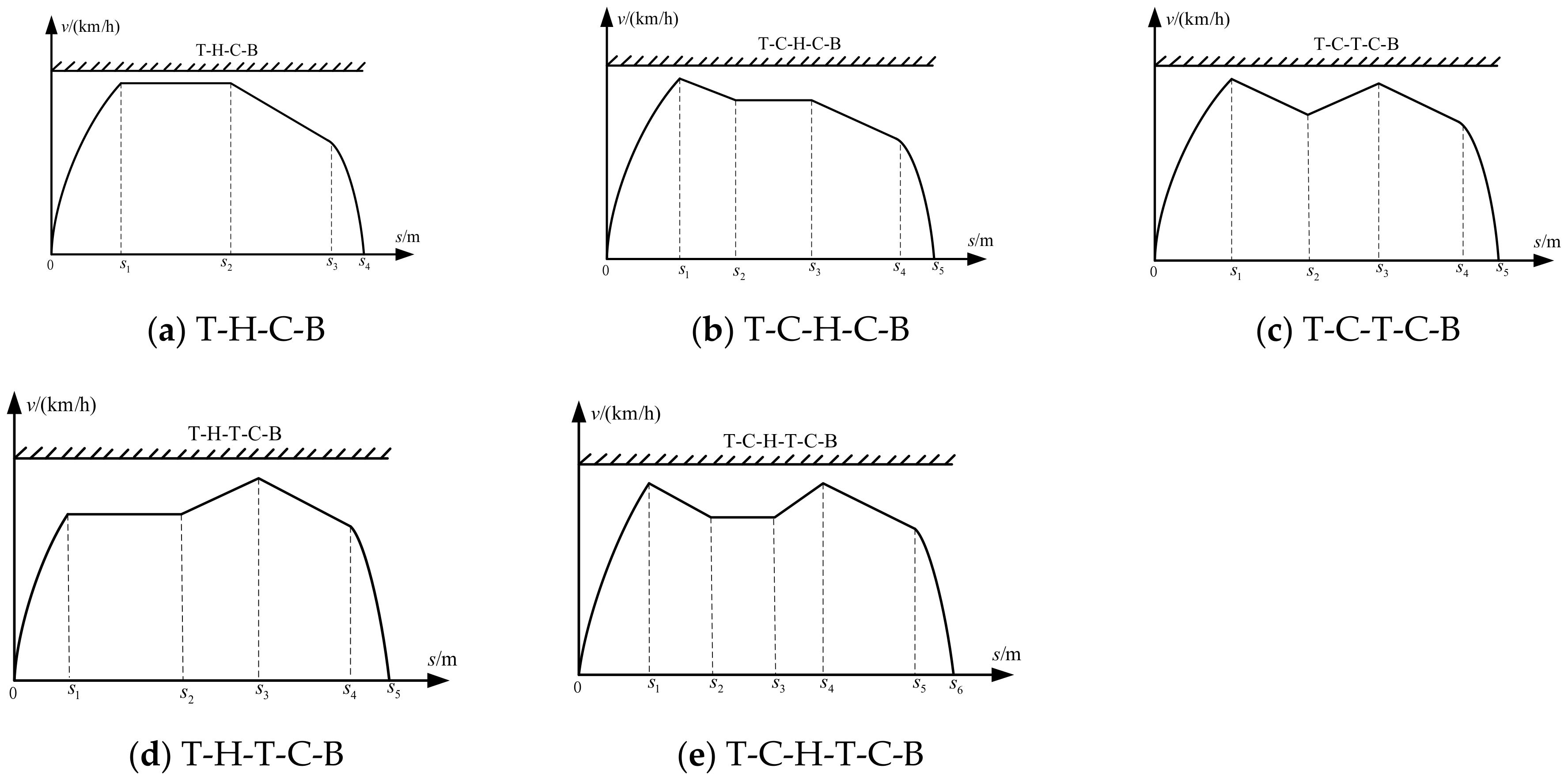
Therefore, the control sequences that violate the principle of condition switching and consume time and energy have been removed, and the following five typical and feasible condition sequences were finally selected for research: ① T-H-C-B; ② T-C-H-C-B; ③ T-C-T-C-B; ④ T-H-T-C-B; ⑤ T-C-H-T-C-B, as shown in Figure 1.

Figure 1. Operation process of 5 typical operating conditions.

3. Model Establishment

3.1. Assumptions and Variables

For the convenience of description, make the following assumptions [9].

(1)

The train is a mass particle, considering the traction and rotation coefficient;

(2)

Stations are abstracted as nodes, and section curves are abstracted as arcs;

(3)

The train can output any traction force not greater than the maximum traction force at the current speed.

3.2. Multi-Objective Model Establishment and Constraints

In the process of urban rail train movement, according to Newton’s second law:

$$F=Ma=F_q-F_b-F_r-F_g-F_c.$$

(1)

In the formula, $F$ is the total force on the train, $M$ is the mass of the train, $a$ is the acceleration of the train, $F_q$ is the traction force of the train, and $F_b$ is the braking force of the train. $F_r=c_0+c_{1}v+c_2{v}^2$ is the basic resistance, $v$ is the running speed of the train, and $c_0$, $c_1$, $c_2$ is the resistance coefficient. The value of the resistance coefficient is different according to different train models.

$F_g=Mg\tan \theta$ is the additional resistance of the slope, and $M$ is the mass of the train. $g$ is the gravitational acceleration, $\theta$ is the incline angle. Considering that the slope of the line is generally very small in reality, $\tan \theta$ can be used to replace $\sin \theta$ in the project.

$F_c=A/R$ is the resistance of the curve, A is the empirical constant for calculating the resistance of the curve (600 in this paper), and $R$ is the radius of the curve.

For the four train operating conditions of traction, braking, coasting, and constant speed, the value range of A is as follows:

$$\left\{\begin{array}{ll}F>0& \mathrm{traction} \mathrm{condition}\\ F=0& \mathrm{constant} \mathrm{speed} \mathrm{condition}\\ F<0& \mathrm{coasting} \mathrm{and} \mathrm{braking} \mathrm{conditions}\end{array}\right..$$

In this paper, time is used as the iterative step length, and the train running distance and speed are expressed as follows:

$$\mathrm{\Delta }s=v_i\mathrm{\Delta }t+{\displaystyle \frac{1}{2}}{a}_i\mathrm{\Delta }{t}^2$$

(2)

$$s_{i+1}=s_i+\mathrm{\Delta }s.$$

(3)

Formulas (2) and (3) are iterative formulas for calculating the train traveling distance. $s_i$ represents the distance after the $i$ iteration, and $a_i$ is obtained by the discrete processing of $a$ in Formula (1). $s_0=0$, $\mathrm{\Delta }t=0.1$.

Similarly:

$$\mathrm{\Delta }v=v_0+a_i\mathrm{\Delta }t$$

(4)

$$v_{i+1}=v_i+\mathrm{\Delta }v.$$

(5)

Equations (4) and (5) represent the calculation formula of train speed $v_i$ at iteration $i$. $v_0=0$, $\mathrm{\Delta }t=0.1$.

Under the constraints of safety, comfort, and accurate parking, the calculation model for solving train energy consumption and running time is as follows.

The inter-station running time is as follows:

$$f_t=\sum \mathrm{\Delta }t=\sum _{k\in K}{\displaystyle {\int }_0^{S_k}(1/v(s))} ds$$

(6)

where $f_t$ is the running time between stations, $k$ is the identification of the calculation section, $K$ is the set of the calculation section, and $S_k$ is the length of the calculation section.

Inter-station energy consumption is as follows:

$$f_e=\sum _{k\in K}({\displaystyle {\int }_0^{s_k^T}{F}_q(v)} ds+{\displaystyle {\int }_0^{s_k^H}{F}_h(v)} ds+{\displaystyle {\int }_0^{s_k^B}{F}_b(v)} ds)$$

(7)

where $S_k^T$, $S_k^H$, $S_k^B$ are, respectively, the traction, constant speed, and braking distances of the calculated section $k$.

In summary, the objective function of train operation is the overall optimization of energy consumption and time, and the optimization problem is formulated as follows:

$$\min =(f_e , f_t).$$

(8)

The constraint conditions are as follows:

$$s. t.=\left\{\begin{array}{l}{v}_0=v_e=0\hfill \\ v_i<v_{\lim }\hfill \\ \left|T\prime -T\right|<10\mathrm{s}\hfill \\ \left|S\prime -S\right|<30\mathrm{cm}\hfill \\ S={\displaystyle \sum _{k\in K}{S}_k=s_k^T+s_k^H+s_k^C+s_k^B}\hfill \end{array}\right.$$

(9)

where $v_0$ and $v_e$ are the starting and ending speeds of the train section; $v_i$ is the speed of the train at a certain time; $v_{\lim }$ is the speed limit of the line; $T\prime$ and $T$ are the interval planning running time and the actual running time, respectively. $S\prime$ and $S$ are the actual distance and actual running distance of the train in the section, respectively. ${\mathrm{s}}_k^C$ is the coasting distance of section $k$.

Therefore, these five typical operating condition sequences are combined in the given urban rail train operation interval. Different working condition sequence combinations correspond to different optimal solutions, and the optimal working condition sequence can be obtained by comprehensive comparison, so as to improve the quality of the optimal solution and optimize the multi-objective operation process.

4. Model Solution

4.1. Pareto Optimization Algorithm Implementation

In this study, NSGA-II is used to search for the optimal Pareto solution set. The NSGA-II algorithm is a fast, non-dominant multi-objective optimization algorithm with an elite retention strategy, which is a multi-objective optimization algorithm based on Pareto optimal solutions [10,11,12,13].

4.1.1. Selection, Crossover, and Mutation

In this paper, the individual encoding method of the genetic algorithm chooses the real number encoding method. In the process of optimization, the quality of an individual depends on the fitness of the individual, and an individual with high fitness is more likely to be retained into the next generation. In practice, fitness is generally an individual objective function.

(1)

Selection

The selection operation imitates the principle of “survival of the fittest” in nature. if the fitness of an individual is high, it has a higher probability of being inherited to the next generation, otherwise the probability is small.

(2)

Crossover

Crossover operation simulates the phenomenon of chromosome transposition in nature and is used to generate new individuals, which determines the global search ability of the algorithm. The standard NSGA-II algorithm uses the analog binary crossover operator, and the calculation formula of the $k+1$ generation individual is as follows [10,11,12,13]:

$$p_{1,k+1}={\displaystyle \frac{1}{2}}[(1-{\beta }_{qi})p_{1,k}+(1+{\beta }_{qi})p_{2,k}]$$

(10)

$$p_{2,k+1}={\displaystyle \frac{1}{2}}[(1+{\beta }_{qi})p_{1,k}+(1-{\beta }_{qi})p_{2,k}].$$

(11)

In Formulas (10) and (11), $p_{1,k+1}$ and $p_{2,k+1}$ are the $k+1$ generation individuals generated after crossing; $p_{1,k}$ and $p_{2,k}$ are selected individuals of generation $k$; and ${\beta }_{qi}$ is the uniform distribution factor, which is calculated as follows:

$${\beta }_{qi}={(2{\mu }_i)}^{{\displaystyle \frac{1}{\eta +1}}},{\mu }_i\le 0.5$$

(12)

$${\beta }_{qi}={\displaystyle \frac{1}{[2(1-{\mu }_i)]\frac{1}{\eta +1}}},{\mu }_i\ge 0.5.$$

(13)

In Formulas (12) and (13), ${\mu }_i$ is a random number belonging to [0,1); $\eta$ is a cross-distribution index, generally defined as 20~30, and the size of $\eta$ will affect the distance between the generated individual and the parent individual.

(3)

Mutation

Mutation manipulation mimics genetic variation in organisms and, like crossover manipulation, is used to produce new individuals. The mutation operator of the standard NSGA-II algorithm is a polynomial mutation operator, and the calculation formula of the $k+1$ generation individual is as follows [10,11,12,13]:

$$p_{k+1}=p_k+(p_k^{\max }-p_k^{\min }){\delta }_k.$$

(14)

In Formula (14), $p_k$ is the selected individual of generation $k$; $p_{k+1}$ is the $k+1$ generation individual obtained by $p_k$ through mutation operation; and $p_k^{\max }$ and $p_k^{\min }$ are the upper and lower bounds of the decision variables, respectively. ${\delta }_k$ is calculated as follows:

$${\delta }_k=\left\{\begin{array}{l}{(2r_k)}^{{\displaystyle \frac{1}{{\eta }_m+1}}}-1\hspace{1em}\hspace{1em}\hspace{1em}\hspace{1em}{r}_k<0.5\\ \hspace{1em}1-{[2(1-r_k)]}^{{\displaystyle \frac{1}{{\eta }_m+1}}}{r}_k>0.5\end{array}\right..$$

(15)

In Formula (15), $r_k$ is the uniformly distributed random number in [0,1], and ${\eta }_m$ is the variation distribution index.

4.1.2. Fast Non-Dominated Sorting

Fast non-dominated sorting is a concept based on Pareto dominance. Assume that if the $k$ objective function is written as $f_i(x)$, where $i$ is any integer in $1,2,\dots ,k$, $j$ is any integer in $1,2,\dots ,k$, but $i\ne j$. If individuals $x_1$ and $x_2$ have $f_i(x_1)<f_i(x_2)$ for any objective function, then individual $x_1$ is said to dominate individual $x_2$; if there is $f_i(x_1)\le f_i(x_2)$ for any objective function, and at least one objective function holds $f_j(x_1)<f_j(x_2)$, $x_1$ is said to weakly dominate $x_2$; if there is both an objective function that makes $f_i(x_1)\le f_i(x_2)$ true and an objective function that satisfies $f_j(x_1)>f_j(x_2)$, then individuals $x_1$ and $x_2$ are said to be non-dominant.

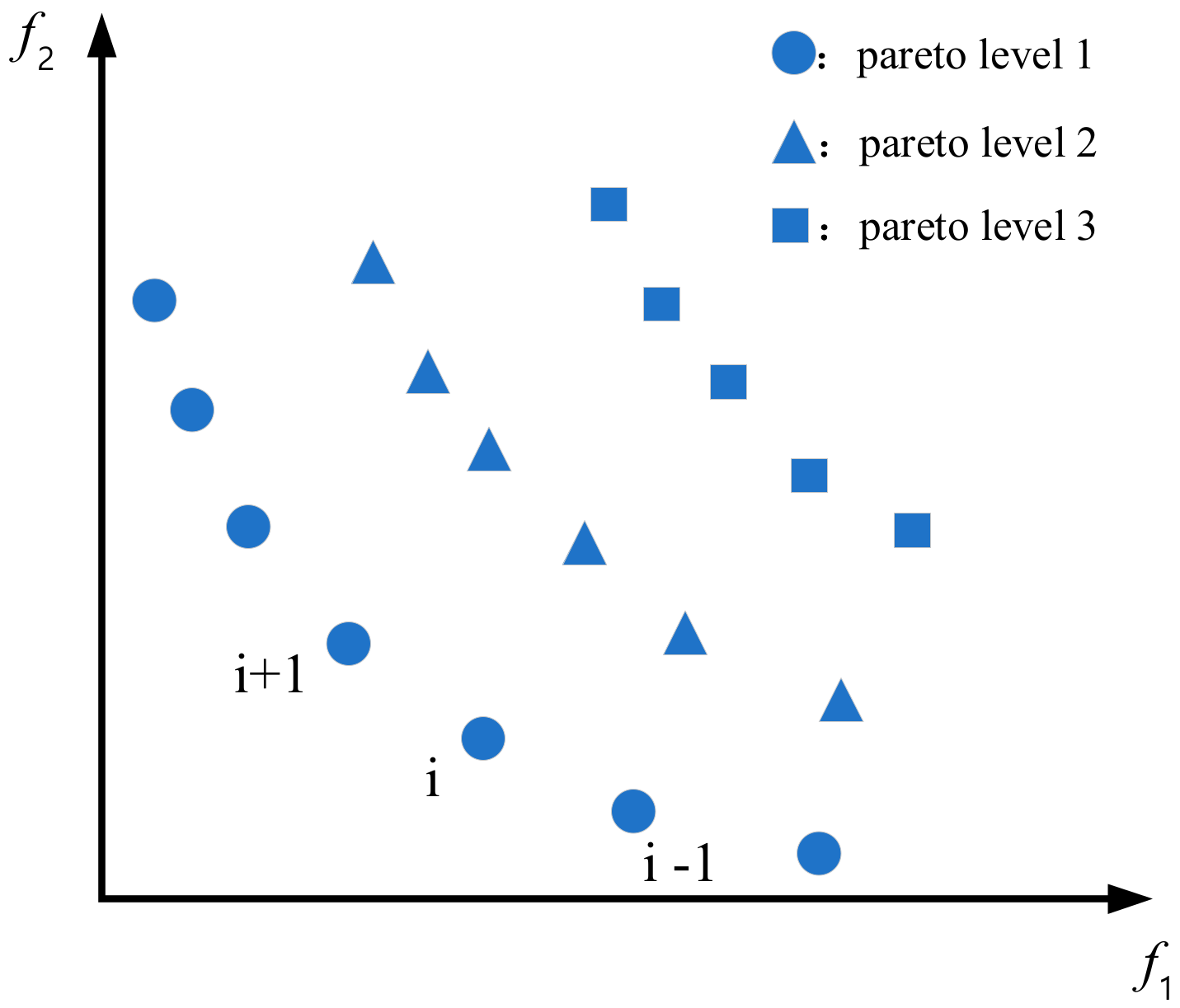
The non-dominant level is also called the Pareto level, in which an individual with a Pareto level of 1 is called the non-dominant solution, also called the Pareto optimal solution, because it is not dominated by other individuals, and the curve formed by the solution set is called the Pareto frontier. For example, there are two objective functions, $f_1$ and $f_2$, and it is assumed that there are three Pareto levels after fast non-dominated sorting, as shown in Figure 2. The individual represented by a circle in Figure 2 is the Pareto optimal solution for this example. That is the set composed of individuals with a Pareto level of 1, and the curve formed by these individuals is the Pareto frontier.

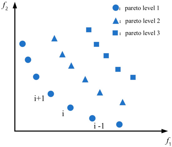
Figure 2. Pareto level frontier optimal solution.

4.1.3. Calculation of Crowding Degree

The degree of crowding represents the density value of an individual in a space, which can be visually represented by a rectangle around an individual that does not include other individuals, as shown in Figure 3.

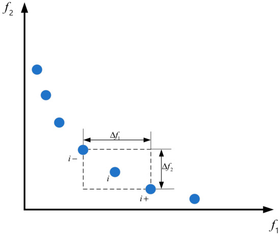
Figure 3. Crowding distance of Pareto level frontier.

Crowding distance:

$$d_i={\displaystyle \sum _{m=1}^M\left|f_m^{i+1}-f_m^{i-1}\right|}$$

(16)

where $d_i$ represents the crowding distance of individual $i$, $i+1$ and $i-1$ are the two entities connected to the Pareto front line of individual $i$. $f_m^{i+1}$ and $f_m^{i-1}$ represent the $m$ objective function values of individuals $i+1$ and $i-1$, respectively.

4.1.4. Elite Strategy

The NSGA-II algorithm introduces an elite strategy to achieve the goal of retaining excellent individuals and eliminating inferior individuals. The elite strategy expands the selection range when producing the next generation of individuals by mixing parent and child individuals to form a new group. Taking the example shown in Figure 4 for analysis, where $P$ represents the parent population—assuming that the number of individuals is $n$—and $Q$ represents the child population, the specific steps are as follows:

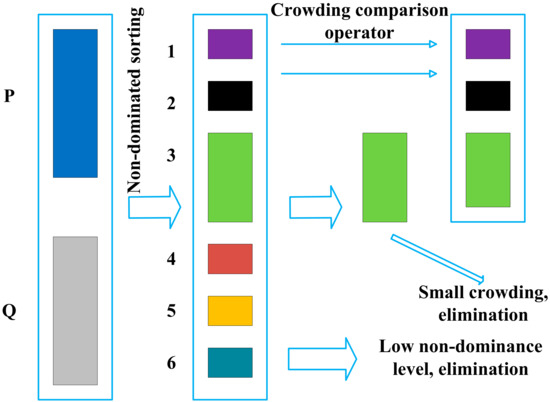
Figure 4. A schematic representation of the elite strategy.

The parent population and child population are merged to form a new population. After that, the new population undergoes non-dominated sorting; in this case, the population is divided into six Pareto levels.

To generate new parents, first put the non-dominant individuals with a Pareto level of 1 into the new parent set, then put the individuals with a Pareto level of 2 into the new parent population, and so on.

If all the individuals of level $k$ are placed in the new parent set, the number of individuals in the set is less than n, and if all the individuals of level $k+1$ are placed in the new parent set, the number of individuals in the set is greater than $n$. The crowding degree is calculated for all individuals at level $k+1$, all individuals are ranked in descending order according to the crowding degree, and then all individuals with a level greater than $k+1$ are eliminated. As can be seen from Figure 4, k is 2, so the crowding degree of individuals with a Pareto level of 3 is calculated and sorted in descending order, and all individuals with a Pareto level of 4 to 6 are eliminated.

The individuals in level $k+1$ are placed into the new parent set one by one according to the order arranged in step 2, until the number of individuals in the parent set is equal to $n$, and the remaining individuals are eliminated.

4.2. Algorithm Implementation Steps

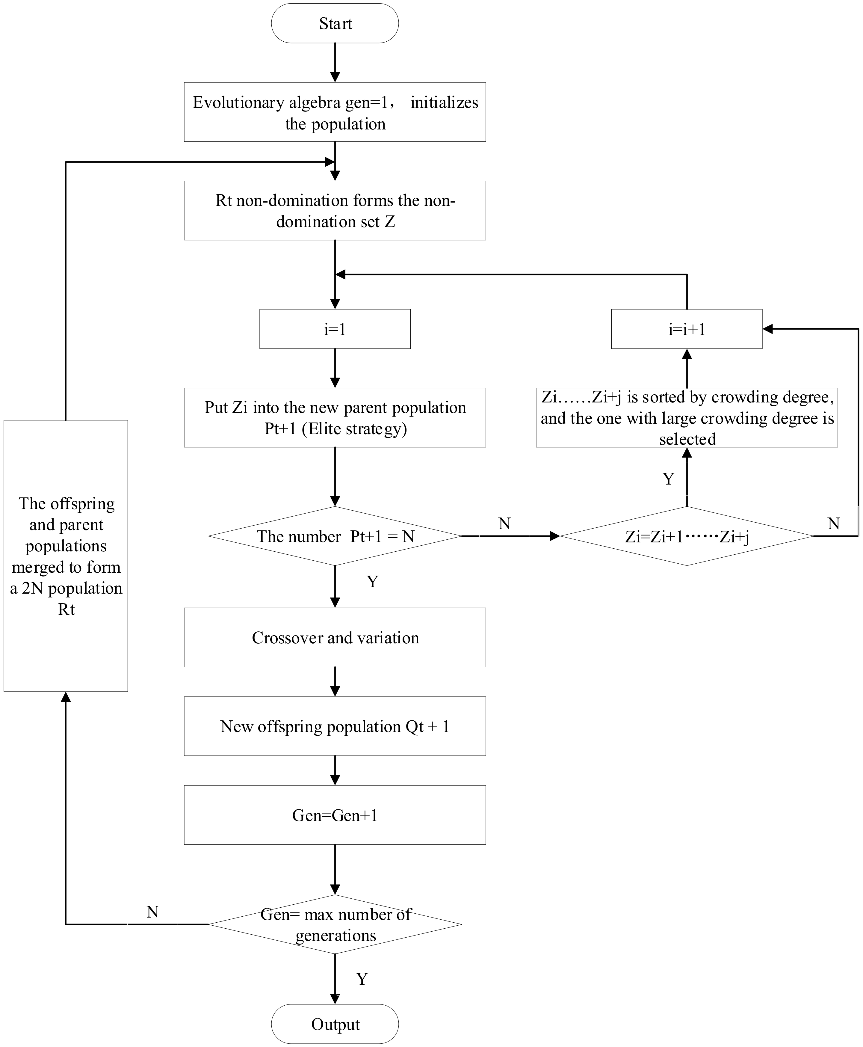
A flowchart of the NSGA-II algorithm is shown in Figure 5, and the specific implementation process is as follows [14]:

Figure 5. Flowchart of NSGA-II algorithm.

Step 1: Initial population and set evolution generation Gen = 1.

Step 2: Determine whether the first generation of the subpopulation is generated—if it is generated, the evolutionary algebra Gen = 2; otherwise, the initial population is generated by non-dominated sorting and selection, Gaussian crossover, and mutation to generate the first generation of the subpopulation, and the evolutionary algebra Gen = 2.

Step 3: Combine the parent population with the child population to form a new population.

Step 4: Determine whether a new parent population has been generated; if not, calculate the objective function of the individuals in the new population, and perform operations such as fast non-dominated sorting, calculation of crowding degree, and elite strategy implementation to generate a new parent population. Otherwise, proceed to step 5.

Step 5: Perform selection, crossover, and mutation operations on the generated parent population to generate the offspring population.

Step 6: Determine whether Gen is equal to the largest evolutionary algebra; if not, then evolutionary algebra Gen = Gen + 1 and return to step 3. Otherwise, the algorithm ends.

4.3. Weight Is Calculated by AHP Mahalanobis Distance Method

In this study, NSGA-II is used to search for the optimum Pareto solution set. The NSGA-II algorithm is a fast non-dominant multi-objective optimization algorithm with an elite retention strategy, which is a multi-objective optimization algorithm based on Pareto optimal solutions [10,11].

The methods of weight distribution include the objective weighting method and the subjective weighting method. The objective weighting method is based on a large amount of data. Generally speaking, it is difficult to obtain data to some extent. However, the subjective weight distribution is mainly dependent on experience and judgment, which inevitably has a certain subjectivity. In this paper, the Mahalanobis distance method of hierarchical analysis, combining the subjective and the objective, is adopted to make the weight distribution of each performance index more reasonable.

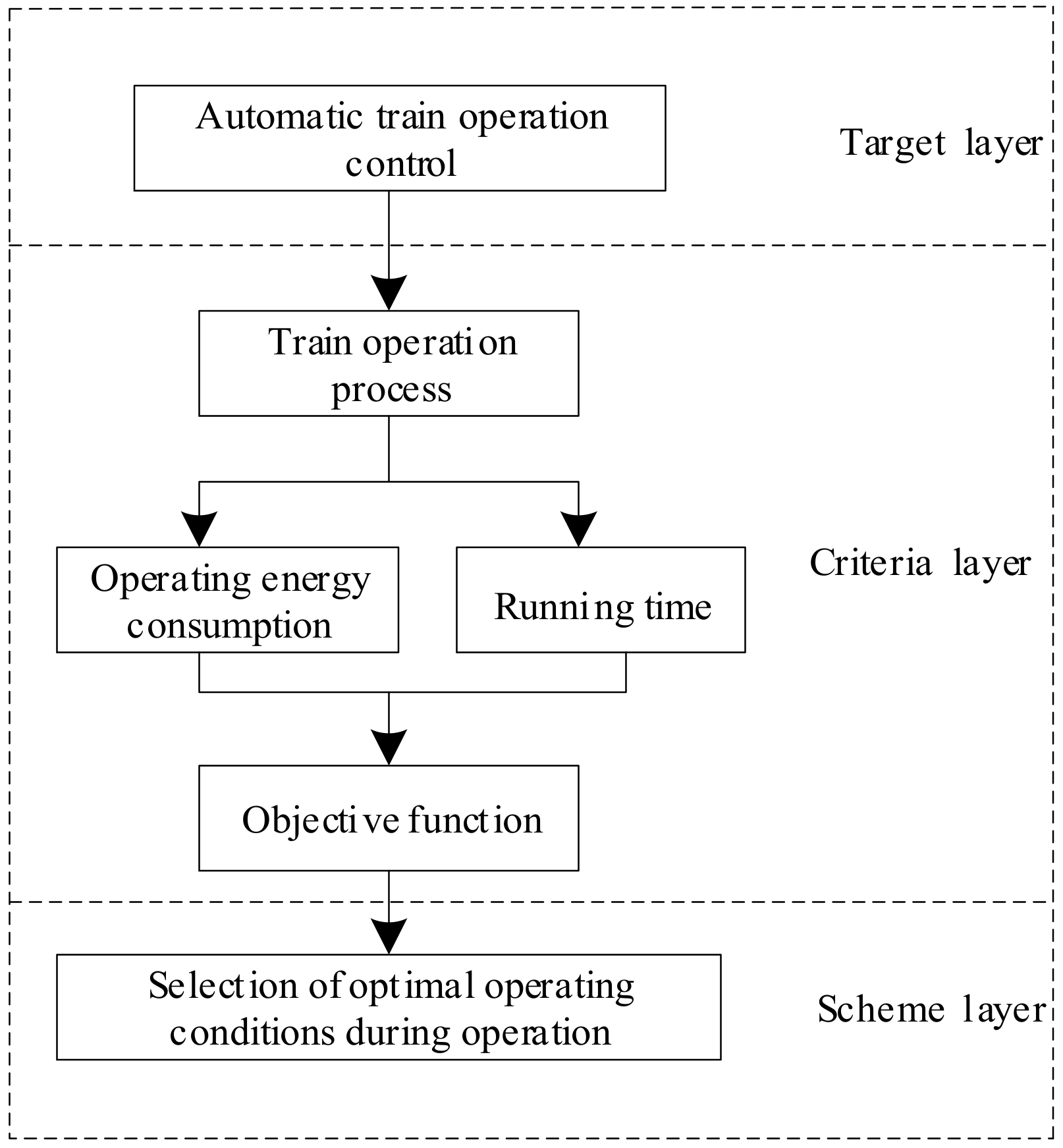
4.3.1. Hierarchical Analysis Model of Train Operation Process

In the hierarchical analysis structure model of automatic train operation control, the target layer is mainly used to achieve the goal of unmanned train operation, the criteria layer takes the performance indicators of the train operation process as the control criteria, and the scheme layer selects the optimal traction operation process condition based on the calculation of the minimum objective function, as shown in Figure 6.

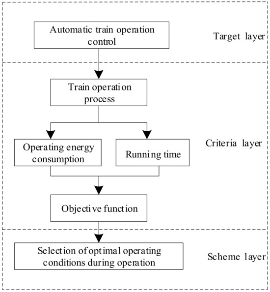
Figure 6. The hierarchical analysis structure model of automatic train operation.

Based on the hierarchical structure model of ATO, the experts have assigned weights to each performance index according to the 1–9 scale method. Each one’s importance has been assigned a number on a scale of 1 to 9, as shown in Table 1. A judgment matrix has also been constructed according to the comparison results of the importance degrees given by the experts for the performance indicators [15,16,17].

Table 1. Definitions and meanings of scale values from 1 to 9.

Scale Value	Definition	Meaning
1	Equally important	Both performance indicators are equally important to a process.
3	Slightly important	Of two performance indicators for a process, one performance is slightly more important than the other performance.
5	Obviously important	Of two performance indicators for a process, one performance is obviously more important than the other performance.
7	Highly important	Of two performance indicators for a process, one performance is highly important compared to the other performance.
9	Extremely important	Of two performance indicators for a process, one performance is extremely important compared to the other performance.
2, 4, 6, 8	Median value of adjacent scale	Represents the scale when there is a compromise between two adjacent scales.
Reciprocal	Reverse comparison	If the scale of performance indicator $i$ to another performance indicator j is $a_{ij}$, otherwise it is $1/a_{ij}$.

In this study, the opinions of four experts regarding train operation have been collected, weight values have been calculated, and the Mahalanobis distance has been used for analysis, so that the weight distribution of each performance index is more objective and reasonable. Taking one expert as an example, the running energy consumption is A1, the running time is A2, and the weight value is $\omega$. The results are shown in Table 2 [15,16,17].

Table 2. Weight values in operation stage.

Index	A1	A2	$\mathit{\omega }$
A1	1	2	0.667
A2	1/2	1	0.333

The average algorithm is adopted for the calculation of $\omega$, as shown in Formula (17).

$$\omega ={\displaystyle \frac{1}{n}}\times {\displaystyle \sum _{j=1}^n(\frac{a_{ij}}{{\displaystyle \sum _{i=1}^n{a}_{ij}}})},i=1,2,3,\cdot \cdot \cdot ,n$$

(17)

Among them, ${\omega }_1$ and ${\omega }_2$ are calculated as follows:

$${\omega }_1={\displaystyle \frac{1}{2}}({\displaystyle \frac{1}{1+1/2}}+{\displaystyle \frac{2}{1+2}})={\displaystyle \frac{2}{3}}=0.667$$

(18)

$${\omega }_2={\displaystyle \frac{1}{2}}({\displaystyle \frac{1/2}{1+1/2}}+{\displaystyle \frac{1}{1+2}})={\displaystyle \frac{1}{3}}=0.333.$$

(19)

Similarly, the weight values of each performance indicator assigned by other experts are calculated as shown in Table 3.

Table 3. Weight values of each performance indicator given by 3 different experts.

Different Experts	Operation Process
	Energy Consumption	Running Time
Expert 1	0.667	0.333
Expert 2	0.75	0.25
Expert 3	0.5	0.5
Expert 4	0.75	0.25

4.3.2. Weight Allocation by Mahalanobis Distance Method

The Mahalanobis distance method represents the covariance distance of data, which is mainly used to measure the similarity between two samples. The set of weight values given by each expert can be regarded as a sample, the weight matrix is constructed, and the Mahalanobis distance value between samples is calculated. The smaller the distance value is, the closer the samples are. Moreover, samples with a large Mahalanobis distance are excluded by comparison, and the final weight value of each performance index is obtained by averaging the remaining samples [15,16,17].

(1)

Build the weight matrix.

According to the analytic hierarchy process, the weight matrix $M$ is composed of the weight values of each performance index in different operation stages, obtained using the experience of four experts. Where $M={({\omega }_{ij})}_{m\times n}$, ${\omega }_{ij}$ represents the weight of the $i$ expert on the $j$ indicator, $m$ is the number of experts, and $n$ is the number of performance indicators.

$$M=\left[\begin{array}{cc}0.667& 0.333\\ 0.75& 0.25\\ 0.5& 0.5\\ 0.75& 0.25\end{array}\right]$$

(20)

(2)

The average weight of each performance index given by each expert is calculated, respectively, and then the covariance $S_1$ is calculated according to the average weight, and finally the corresponding inverse matrix $S_1^{-1}$ of the covariance matrix is obtained.

(3)

Calculate Mahalanobis distance. The similarities between the weights determined by different experts can be calculated according to different running stages. The calculation formula is as follows:

$$D_{ij}=\sqrt{{(Q_i-Q_j)}^T{S}^{-1}(Q_i-Q_j)}$$

(21)

where $D_{ij}$ represents the Mahalanobis distance value between the weights of performance indicators given by expert $i$ and expert $j$, $Q_i$ and $Q_j$ represent the weight value of each performance indicator given by expert $i$ and expert $j$, respectively. As shown in Table 4.

Table 4. Mahalanobis distance values between experts during train operation.

Distance	Expert1	Expert2	Expert3	Expert4	The Mahalanobis Distance Value of the Population
Expert 1	0.0000	1.7468	2.2515	1.8395	5.8378
Expert 2	1.7468	0.0000	3.4242	0.1660	5.3370
Expert 3	2.2515	3.4242	0.0000	3.5697	9.2454
Expert 4	1.8395	0.1660	3.5697	0.0000	5.5752

(4)

Determine the final weight value.

The smaller the Mahalanobis distance, the greater the similarity. According to the Mahalanobis distance values of the different experts in the braking stop stage, obtained using the above calculation, Expert 3 is excluded from the braking stop stage because the Mahalanobis distance value of Expert 3 is the largest. Then the remaining three groups of expert weights are rearranged to calculate the average value, so as to obtain the weights of each index after optimization by the Mahalanobis distance method.

$${\omega }_j={\displaystyle \frac{1}{p}}{\displaystyle \sum _{i=1}^p{\omega }_{ij},(j=1,2,\cdot \cdot \cdot ,n)}$$

(22)

It can be calculated that the index weight of the braking stop stage is ${\omega }_3=(0.3542,0.6458)$.

In the process of ATO, the weights of each performance index in each stage are calculated as shown in Table 5.

Table 5. Weight values of each performance indicator.

	Train Operation Process
Performance Indicator	Energy Consumption	Running Time
Weight	0.7223	0.2777

4.4. Multi-Objective Optimal Solution

In order to eliminate the incommensurability caused by different unit dimensions, the objective function response data energy consumption and running time need to be processed:

$$x_{ij}^{*}(r)={\displaystyle \frac{x_{ij}(r)-x_{ij,\min }(r)}{x_{ij,\max }(r)-x_{ij,\min }(r)}}.$$

(23)

Multi-objective optimization solution value:

$$f_{\min }={\omega }_1{f}_e+{\omega }_2{f}_t.$$

(24)

5. Experimental Simulation and Result Analysis

5.1. Simulation Parameter Setting

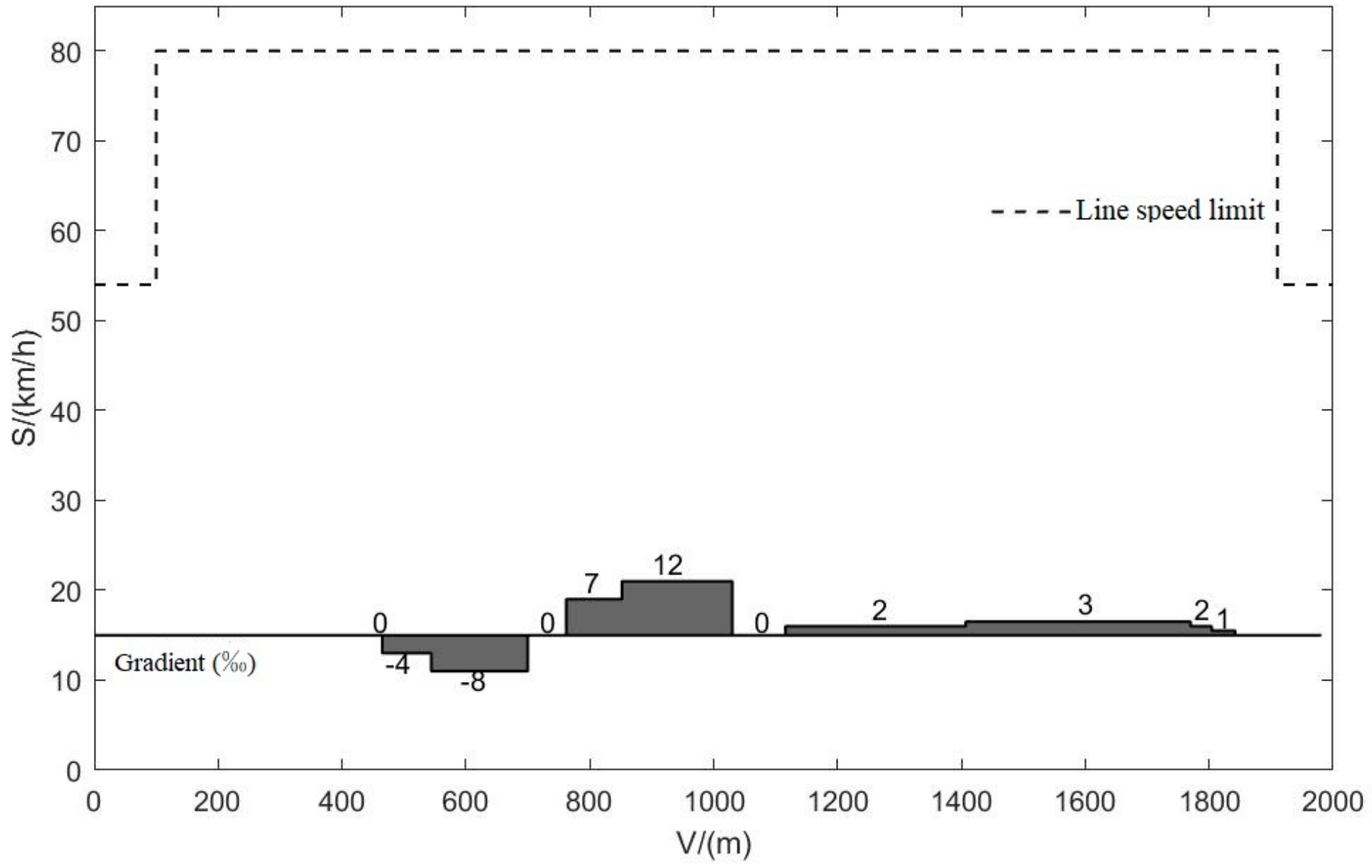
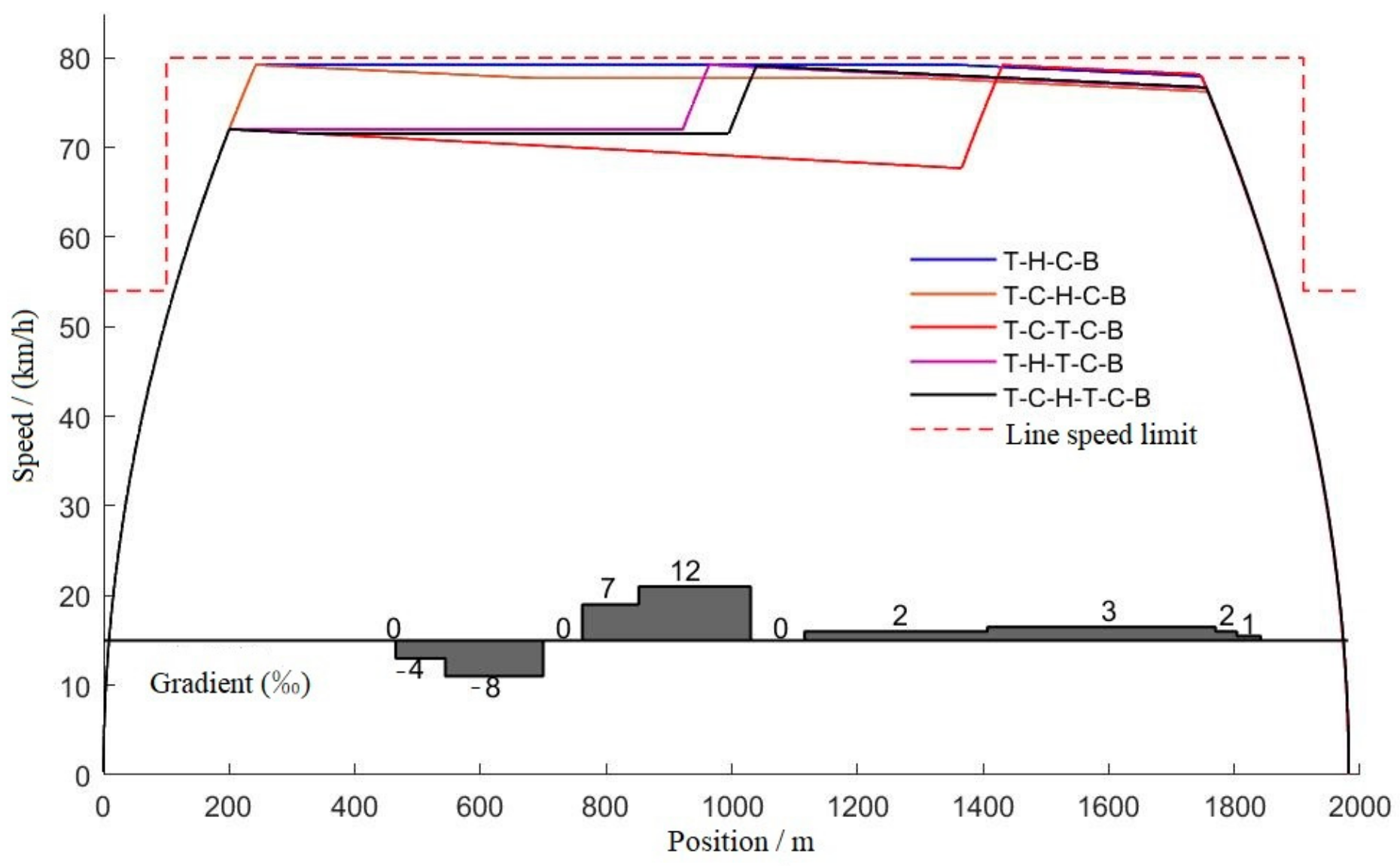
In order to verify the effectiveness of the NSGA-II algorithm, the Beijing Yizhuang subway line of Guangong station—the Yizhuang Bridge station line—is taken as an example. The length between stations is 1982 m, the maximum travel planning time is 129 s, the sampling time step is 0.1 s, and the speed limit and slope information of the line are shown in Figure 7 [18,19]. The simulation is implemented through MATLAB/Simulink2020b programming. The hardware environment of the simulation is an Intel^®Core™i7-11800H@2.30 GHzCPU and the memory is 16.0 GB.

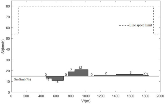
Figure 7. Line speed limit and gradient information.

Taking the DKZ32 Beijing Metro Type B train as an example, the train and control parameters are shown in Table 6 [18,19].

Table 6. Simulated train parameters.

Name	Parameter Value
Train weight/(t)	200
Maximum speed/(km/h)	80
Maximum traction acceleration/(m/s2)	1
Maximum braking acceleration/(m/s2)	1
Basic operating resistance parameters	$c_0=2.031,c_1=0.0622v,c_2=0.001807$

During the parameter setting of the NSGA-II algorithm simulation, the parameter paretoFraction dictates that the optimal individual coefficient is 0.3; populationsize determines that the population size is 100; generations dictates that the maximum evolutionary algebra is 200; stallGenLimit stops the algebra at 200; and TolFun determines that the fitness function deviation is 1 × 10⁻¹⁰.

5.2. Simulation Verification and Analysis

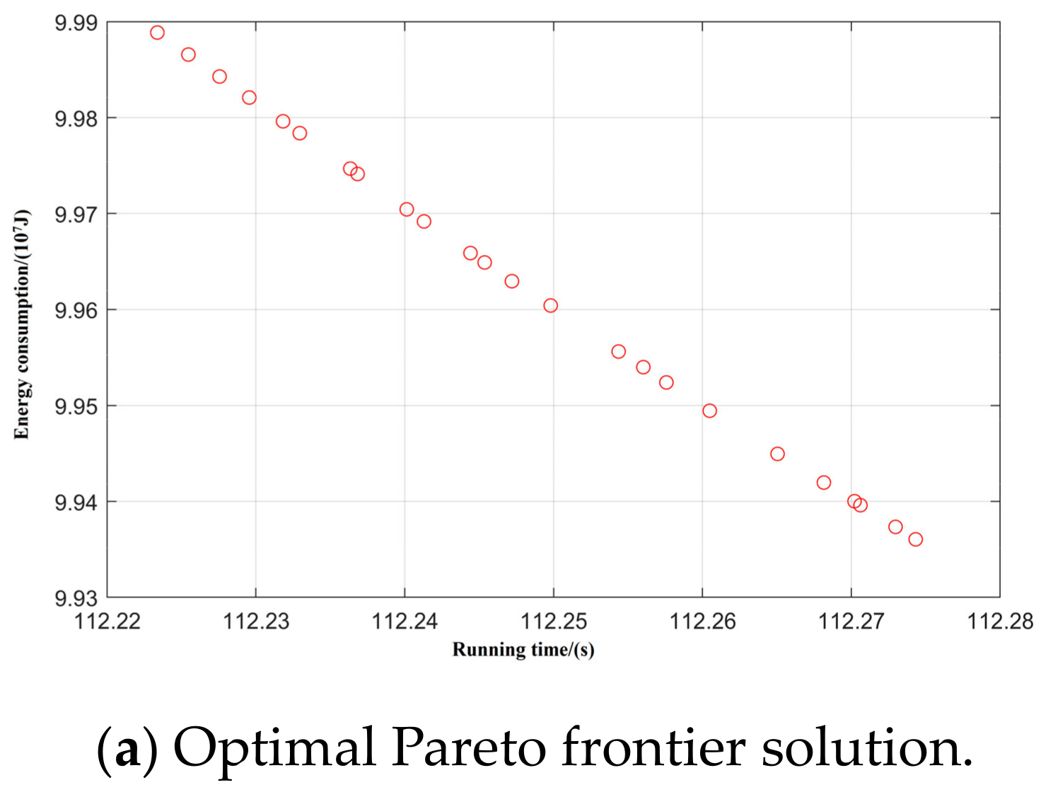
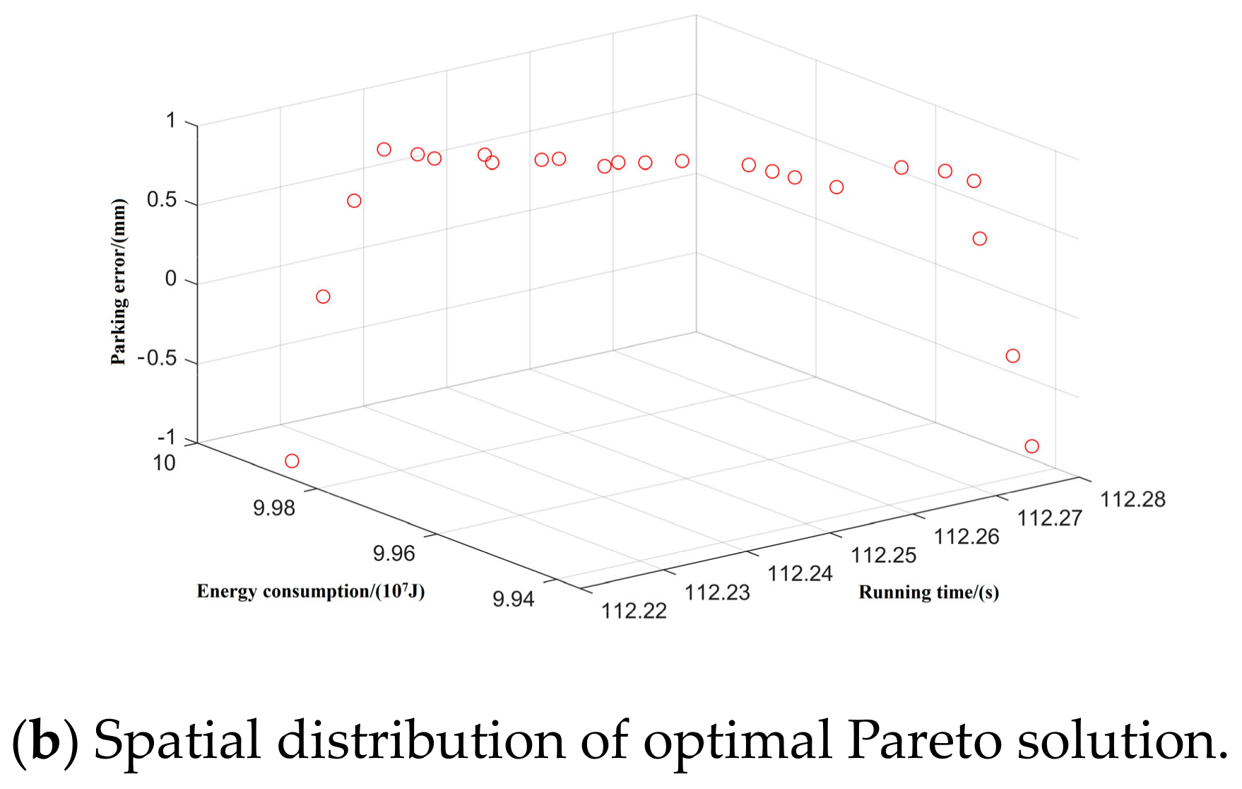
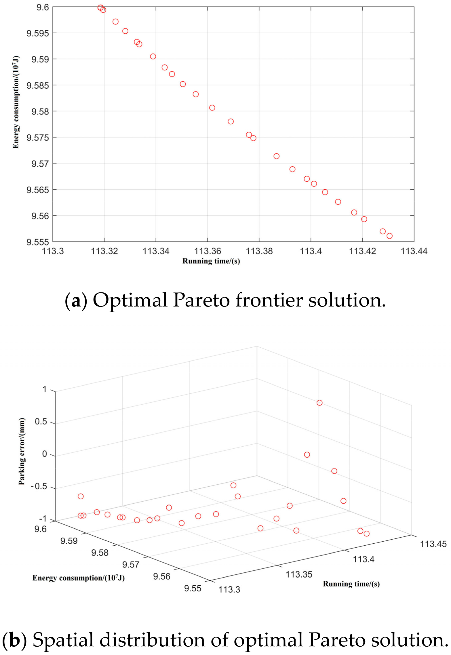
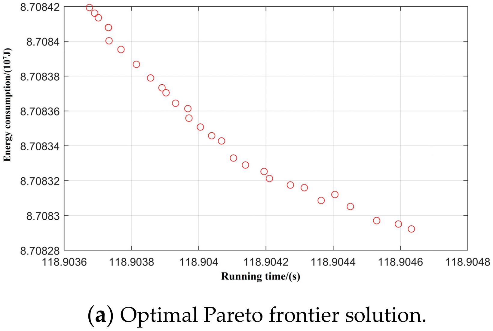
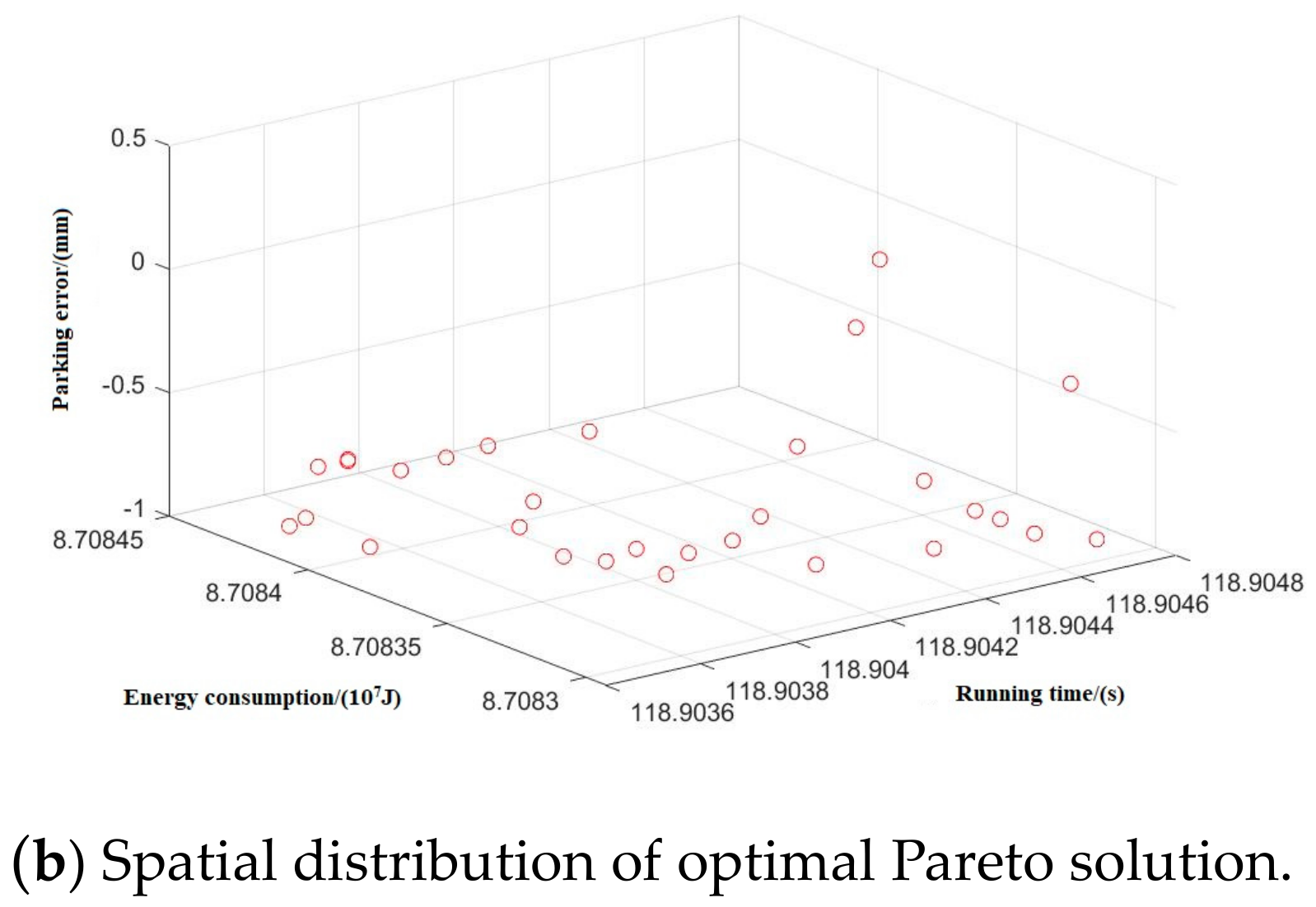
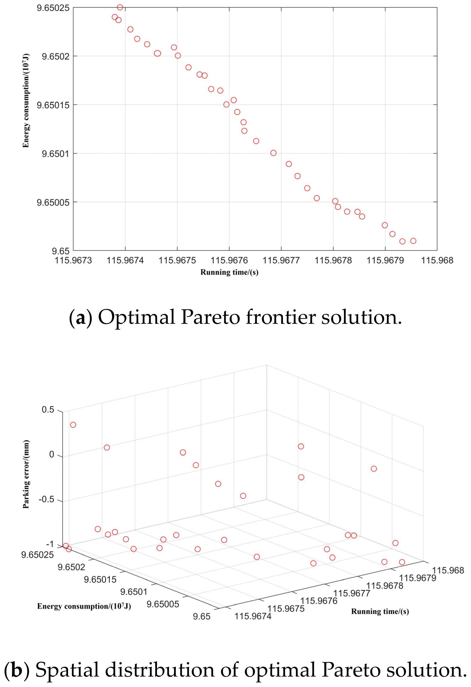
Taking inter-station running time, running distance, and energy consumption as the control objectives, NSGA-II was used to search for the optimal Pareto multi-objective solution set. The simulation results are shown in Figure 8, Figure 9, Figure 10, Figure 11 and Figure 12:

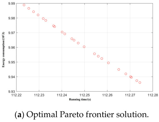
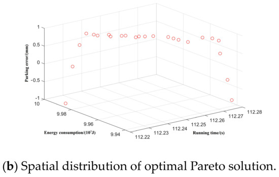
Figure 8. Spatial distribution of Pareto edge solution and optimal solution under T-H-C-B working condition sequence.

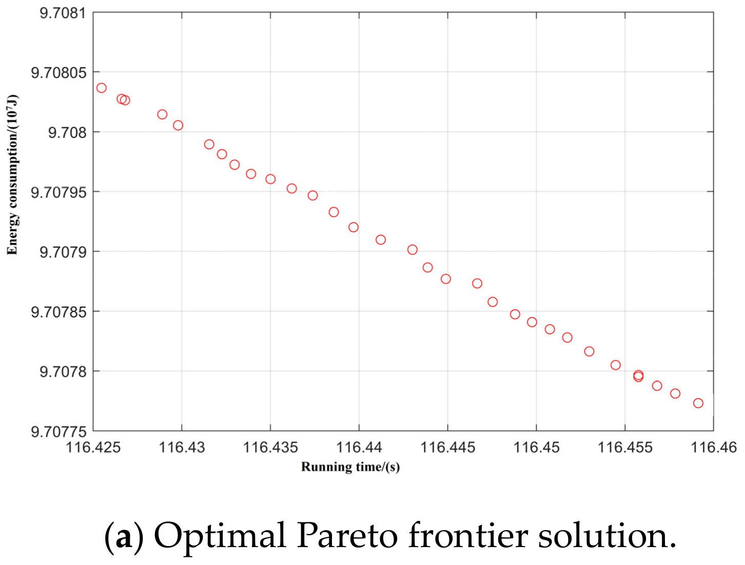
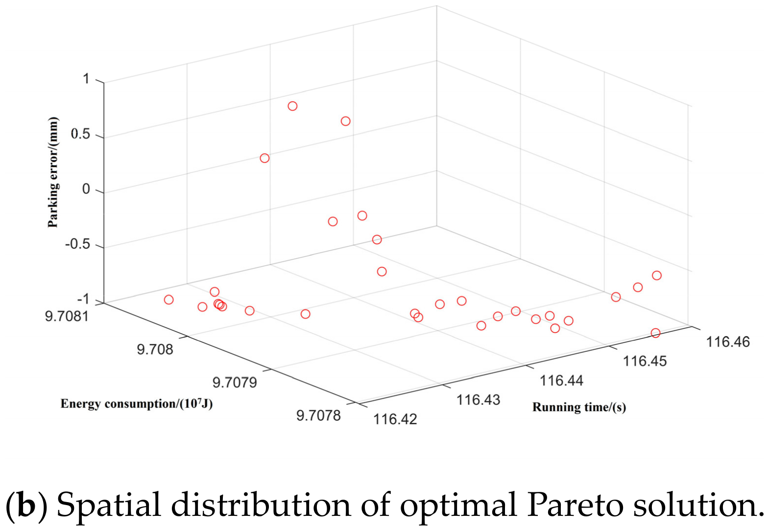
Figure 9. Spatial distribution of Pareto edge solution and optimal solution under T-C-H-C-B working condition sequence.

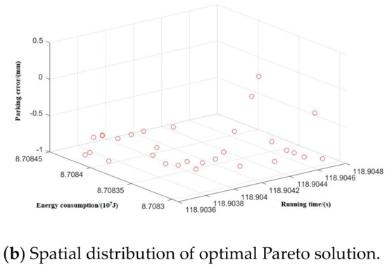
Figure 10. Spatial distribution of Pareto edge solution and optimal solution under T-C-T-C-B working condition sequence.

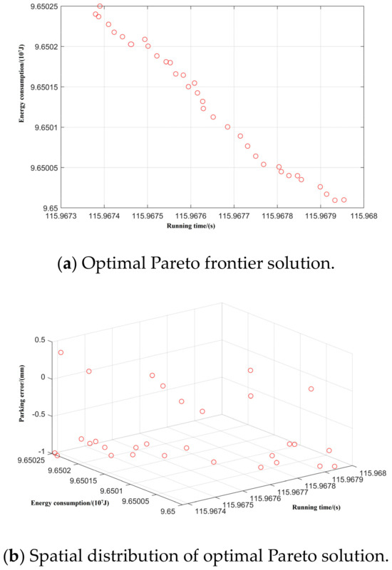
Figure 11. Spatial distribution of Pareto edge solution and optimal solution under T-H-T-C-B working condition sequence.

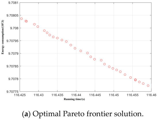
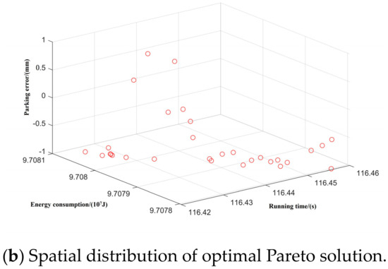
Figure 12. Spatial distribution of Pareto edge solution and optimal solution under T-C-H-T-C-B working condition sequence.

By optimizing the Pareto frontier solution set for each working condition, the optimal values of the five typical working condition sequences are obtained, as shown in Table 7.

Table 7. Optimal values of 5 typical working condition sequences.

Sequence of Operating Conditions	Distance of Operation S (m)	Energy Consumption E (×107 J)	Running Time T (s)	Operation Time of Each Working Condition (s)
T-H-C-B	1982	9.98	112.2	22-50.8-17.8-21.6
T-C-H-C-B	1982	9.57	113.4	22-20.5-28.7-21-21.2
T-C-T-C-B	1982	8.71	118.9	20-60.1-3.2-14.4-21.7
T-H-T-C-B	1982	9.65	115.9	20-36.1-2-36.6-21.3
T-C-H-T-C-B	1982	9.71	116.4	20-6.5-33.3-2.1-33.1-21.3

Through the optimal solution of the five typical working condition sequences, their optimal velocity–distance curves are obtained by the simulation; these are shown in Figure 13.

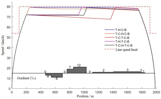
Figure 13. Optimal velocity–distance curves of 5 typical operating sequences.

Through comparative analysis it can be seen that, using the premise of ensuring the accuracy of parking, each condition sequence can meet the requirements of the operating conditions. The T-C-T-C-B condition sequence has the least energy consumption, which is 12% lower than the T-H-C-B condition sequence, which has the most energy consumption. The interval running time of the T-C-T-C-B working condition sequence is the longest, being 7.2 s longer than that of the T-H-C-B working condition sequence, which has the shortest running time; both of these meet the requirement of 129 s less than the maximum running time. The excess time can be added to the coast condition in later running, and further decrease the energy consumption of train operation. The remaining three typical operating conditions are intermediate in energy consumption and running time.

At the same time, the choice of the optimal working condition will be different due to the different lengths of the lines and the rail conditions.

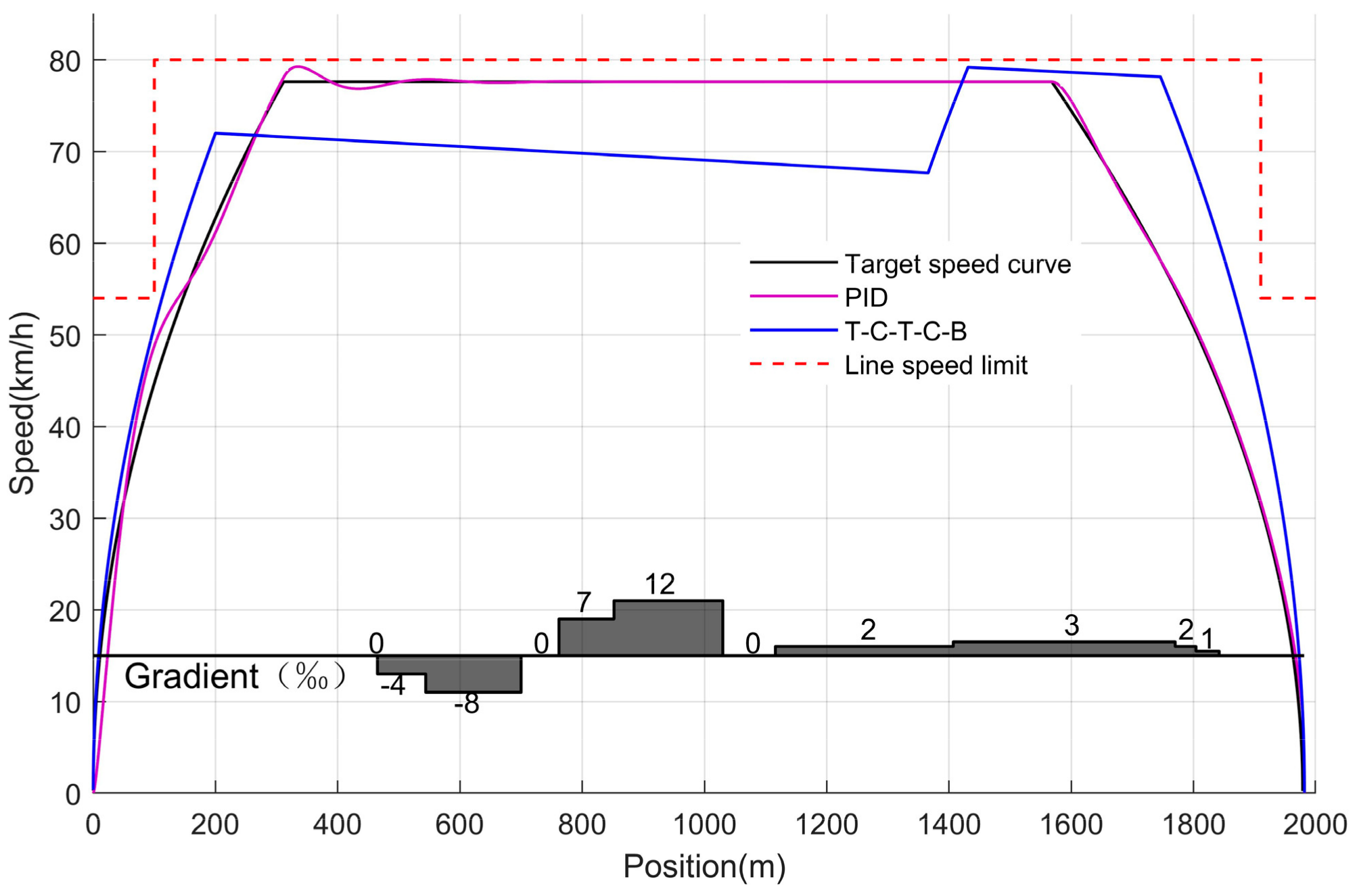
If the conditions of parking accuracy and running time are comprehensively considered, all the five working condition sequences can meet the operating requirements, but the T-C-T-C-B working condition sequence has the least energy consumption, making it the optimal working condition sequence combination under the experimental conditions. The optimal operating condition is compared with the traditional PID control, and the specific operation process is shown in Figure 14.

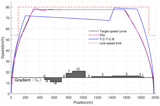
Figure 14. The velocity–distance curves corresponding to the T-C-T-C-B condition sequence and PID control.

The simulation results of the T-C-T-C-B condition sequence and the traditional PID algorithm regarding train running time, parking accuracy, and operation energy consumption are shown in Table 8.

Table 8. A comparison of the optimal working condition sequence with the traditional PID control algorithm.

Algorithm	Running Time T (s)	Distance of Operation S (m)	Energy Consumption E (×107 J)
T-C-T-C-B	118.9	0	8.71
PID	128.5	0.137	10.4

It can be seen from the table that although the traditional PID control algorithm realizes the accurate control of trains during ATO by tracking the given target speed curve, there is a certain deviation between the speed curve and the target speed curve under the PID algorithm, and there is a certain error between the actual stopping position of the train and the target distance, which also increases the train operation energy consumption. Using the optimal planning of the T-C-T-C-B operating condition sequence, the accuracy of train stopping operations is enhanced, the running time between stations is decreased, and the energy consumption of trains is reduced.

6. Discussion and Conclusions

In this paper, the NSGA-II multi-objective optimization algorithm is used to solve the speed curve optimization problem of urban rail trains in five typical operating conditions, and the optimal Pareto multi-objective solution set is searched for. A hierarchical analysis is also carried out using the Mahalanobis distance method, combining the subjective and the objective to assign the weight of the optimal solution. Compared with a single working condition sequence, the solutions under multiple working condition sequences have obvious advantages in terms of quantity and quality, and a large number of high-quality automatic train driving strategies can be obtained. Through the simulation analysis of domestic subway lines, the optimal speed–distance curve is obtained and compared with the traditional PID algorithm, and the effectiveness of the algorithm is verified. This research is important for the intelligent development of urban rail transit. At the same time, it can provide a new basis and method for the multi-objective curve optimization of urban rail automatic driving.

This paper analyzes five typical urban rail transit train operation sequences, which may not cover all train operation conditions, thus limiting the application of the algorithm in a broader range of conditions. At the same time, the operation control performance of the algorithm in complex and variable environments needs to be studied further.

References

- Xu, K.; Yang, F.; Tu, Y.; Wu, S. Multi-objective optimization of urban rail train speed curve based on multi-particle swarm collaboration. J. Railw. 2021, 43, 95–102. [Google Scholar]
- Li, C.; Wang, X.M. ATO control strategy based on particle swarm optimization. J. China Railw. Soc. 2017, 39, 53–58. [Google Scholar]
- Shang, G.W.; Yan, X.; Cai, B.; Wang, J. Multiobjective optimization for train speed trajectory in CTCS High-Speed Railway with hybrid Evolutionary Algorithm. IEEE Trans. Intell. Transp. Syst. 2015, 16, 2215–2225. [Google Scholar] [CrossRef]
- Yang, H.; Liu, H.; Fu, Y. Multi-objective operation optimization for electric multiple unit-based on speed restriction mutation. Neurocomputing 2015, 169, 383–391. [Google Scholar] [CrossRef]
- Dullinger, C.; Struckl, W.; Kozek, M. Simulation-based multi-objective system optimization of train traction systems. Simul. Model. Pract. Theory 2017, 72, 104–117. [Google Scholar] [CrossRef]
- Fernández-Rodríguez, A.; Fernández-Cardador, A.; Cucala, A.P. Real time eco-driving of high speed trains by simulation-based dynamic multi-objective optimization. Simul. Model. Pract. Theory 2018, 84, 50–68. [Google Scholar] [CrossRef]
- Eskandarian, A. Scanning the issue. IEEE Trans. Intell. Transp. Syst. 2024, 25, 2174–2181. [Google Scholar] [CrossRef]
- Rajabighamchi, F.; Hajlou, E.M.H.; Hassannayebi, E. A Multi-objective Optimization Model for Robust Skip-Stop Scheduling with Earliness and Tardiness Penalties. Urban Rail Transit 2019, 5, 172–185. [Google Scholar] [CrossRef]
- Zhang, H.; Jia, L.; Wang, L. Study on Generation of Energy-saving Driving Curves of High-speed Train Based on Pareto Multi-objective Optimization. J. China Railw. Soc. 2021, 43, 85–91. [Google Scholar]
- Zhang, D.; Li, J.; Wei, W.; Meng, W.; Zhang, H. Dynamic design optimization of a vibration isolation installation system of a turboprop engine. Mech. Excell. 2022, 44, 581–587. [Google Scholar]
- Chang, H.P.; Li, W.Y.; Dong, F.G.; Guo, X.P. Multi-objective optimization of cold chain logistics distribution path based on NSGA-II. J. Transp. Sci. Technol. Econ. 2022, 24, 2. [Google Scholar]
- Deb, K.; Pratap, A.; Agarwal, S.; Meyarivan, T. A fast and elitist multiobjective genetic algorithm: NSGA-II. IEEE Trans. Evol. Comput. 2002, 6, 182–197. [Google Scholar] [CrossRef]
- Qu, J.; Zhang, C.; Zhang, J. Machining trajectory fitting algorithm based on NSGA-II and least squares principle. Precis. Manuf. Autom. 2019, 02, 25–28. [Google Scholar] [CrossRef]
- Ding, L.; Li, S. Research on RFID enterprise valuation based on double-precision neural network. Stat. Decis. 2012, 21, 76–80. [Google Scholar] [CrossRef]
- Meng, J.; Xu, R.; Li, D.; Chen, X. Combining the Matter-Element model with the associated function of performance indices for automatic train operation algorithm. IEEE Trans. Intell. Transp. Syst. 2019, 20, 253–263. [Google Scholar] [CrossRef]
- Li, L. Research on train automatic driving algorithm based on extenics. Railw. Comput. Appl. 2013, 22, 1–4. [Google Scholar]
- Zhang, C.; Liu, X. Research on performance index weight allocation scheme of automatic train operation system. Railw. Commun. Signal. 2012, 48, 9–12. [Google Scholar]
- Su, S.; Tang, T.; Li, X. Driving strategy optimization for trains in subway systems. Proc. Inst. Mech. Engineers. Part F J. Rail Rapid Transit 2016, 232, 369–383. [Google Scholar] [CrossRef]
- Chen, X.; Guo, X.; Meng, J.; Xu, R.; Li, S.; Li, D. Research on ATO Control Method for Urban Rail based on Deep Reinforcement Learning. IEEE Access 2023, 11, 5919–5928. [Google Scholar] [CrossRef]
Disclaimer/Publisher’s Note: The statements, opinions and data contained in all publications are solely those of the individual author(s) and contributor(s) and not of MDPI and/or the editor(s). MDPI and/or the editor(s) disclaim responsibility for any injury to people or property resulting from any ideas, methods, instructions or products referred to in the content. |
© 2024 by the authors. Licensee MDPI, Basel, Switzerland. This article is an open access article distributed under the terms and conditions of the Creative Commons Attribution (CC BY) license (https://creativecommons.org/licenses/by/4.0/).