Interpretable Support Vector Machine and Its Application to Rehabilitation Assessment

Abstract

This paper does present an interpretable support vector machine (SVM) and its application to rehabilitation assessment. We introduce the concept of nearest boundary point to standardize the one-class SVM decision function and determine the shortest path for data from abnormal cases to become those from normal cases. This analytical approach is computationally simple and provides a unique solution. The nearest boundary point of abnormal data can also be used to analyze the cause of abnormal classification and indicate countermeasures for normalization. These properties render the proposed interpretable SVM valuable for medical assessment applications and other problems that require careful consideration of classification results for treatment. Simulation and application results demonstrate the feasibility and effectiveness of the proposed method.

1. Introduction

Recently, machine learning (ML) has been applied to various fields, and its classification algorithms have demonstrated high performance. ML has been actively used in the medical industry, particularly in medical imaging [1,2], and in health metric analyses and predictions [3].

There is a wide range of methods available for assessing muscle function in rehabilitation patients. However, traditional techniques such as manual muscle testing (MMT) provide limited detailed information about muscle function and fail to identify the underlying factors contributing to muscle dysfunction. Additionally, treatment approaches for patients with impaired muscle function are often generalized and not tailored to individual needs. This lack of specificity in both assessment and intervention highlights a significant gap in personalized rehabilitation strategies, underscoring the need for more comprehensive and precise methods to evaluate and address muscle function deficits.

We aimed to develop a classification method that can replace various assessment methods for patients undergoing rehabilitation and performed analysis based on the results obtained from a classification method to establish patient treatment plans. To this end, we formulated the following research questions:

• How can we handle the imbalance between data from normal and abnormal cases? One challenge in applying ML to healthcare is the imbalance between data from normal and abnormal cases. It is easier to obtain data from normal individuals than from patients presenting specific health conditions, and not all patient data are abnormal. Consequently, accurately labeling abnormality may be challenging.
• How can we use patient treatment plans considering classification results? In addition to achieving a high classification performance, developing an interpretable classifier is crucial for applying the results to support patient treatment planning. The classifier interpretability may increase trust and usability, thus facilitating the development of treatment plans based on classification results.

The first research question focuses on addressing the issue of data imbalance, where the dataset contains two classes—normal and abnormal—with the abnormal class significantly underrepresented. To tackle this imbalance, several approaches have been considered. One approach is the synthetic minority over-sampling technique (SMOTE) [4], which resamples the minority (rare) class. Another approach is an ensemble method, where the majority (abundant) class is split into smaller subsets, each of which is then trained with the entire rare class to create multiple models, which are subsequently combined [5]. A third method involves clustering the abundant class and training only on representative values (e.g., medians) of these clusters [6].

However, these methods have limitations when applied to our context, where the imbalance is severe. The SMOTE technique is less effective because it requires identifying the distribution pattern of the rare class, which is challenging when the class is extremely underrepresented. Similarly, ensemble and clustering methods are not suitable for our case, as they effectively reduce the amount of data used for modeling, which is problematic given our already limited dataset.

Given these challenges, we chose to address the anomaly detection problem by adopting a one-class classification approach. This method involves training the model exclusively on the abundant class and classifying the remaining data as belonging to the rare class. This approach is particularly well suited to our scenario, as it allows for robust detection of anomalies despite the significant data imbalance.

Several methods have been developed to perform the one-class classification [7,8], from which we used a one-class support vector machine (SVM) [9]. This type of SVM is well-suited for anomaly detection, which identifies datapoints that differ substantially from most of the data. It captures the data distribution and identifies outliers. Another advantage of the one-class SVM is its ability to handle imbalanced datasets, where one class is represented by drastically fewer samples than another one. The one-class SVM can handle situations in which only positive samples are available and negative samples are unknown or difficult to obtain. Hence, it is adequate for medical assessments, especially when collecting data from patients with rare conditions is challenging.

To address the second research question, we devised the nearest boundary point (NBP) to solve for the shortest Mahalanobis distance. Specifically, based on the decision function of the one-class SVM formulated as a mixture of normal distributions, we standardized and analytically derived a series of steps to obtain and reconstruct the NBP. The analytically derived solution is computationally simple and yeilds a unique solution, making it particularly valuable for our rehabilitative assessment application.

To validate the feasibility and applicability of the proposed method, we first performed simulations using artificially generated two-dimensional (2D) nonlinear data. We chose 2D data because they allow for easy visualization and understanding of intermediate steps in addition to verification. After analyzing the simulation results, we tested the proposed interpretable SVM on real data. We trained the one-class classification model on biosensing measurements from normal individuals and classified patient data to solve the NBP problem for identified abnormal data. We analyzed the major factors causing abnormal classifications and investigated feasible treatment methods.

The remainder of this paper is organized as follows. In Section 2, we introduce an interpretable one-class SVM with Gaussian kernels. Section 3 presents the simulation results, and Section 4 reports the analysis of an application to rehabilitation based on the proposed method, including the identification of the main factors and corresponding treatment options for patients classified as abnormal. The simulation and application results validate the effectiveness and interpretability of the proposed SVM. Finally, Section 5 presents our concluding remarks.

2. The Interpretable One-Class SVM

2.1. One-Class Classification of Normally Distributed Data

We address one-class classification as a research question. One-class classification detects anomalies by defining the boundary that encloses normal data. In this subsection, we discuss the case of normal data that follow a normal distribution.

The probability density function of data that following a normal distribution is expressed as

$$\varphi \left(\mathbf{z}\right|\mu ,\Sigma )={\displaystyle \frac{1}{{\left(2\pi \right)}^{d/2}{|\Sigma |}^{1/2}}}exp\left\{-{\displaystyle \frac{1}{2}}{(\mathbf{z}-\mu )}^{\mathbf{T}}{\Sigma }^{-\mathbf{1}}(\mathbf{z}-\mu )\right\},$$

(1)

where $\mu$, $\Sigma$, and d denote the mean, covariance, and dimension of $\mathbf{z}$, respectively.

When data follow a normal distribution, an appropriate boundary can be determined by fitting the data to a normal distribution with a certain mean and covariance and then obtaining the contour of the probability density function, which can be determined by a desired acceptance rate or other approaches.

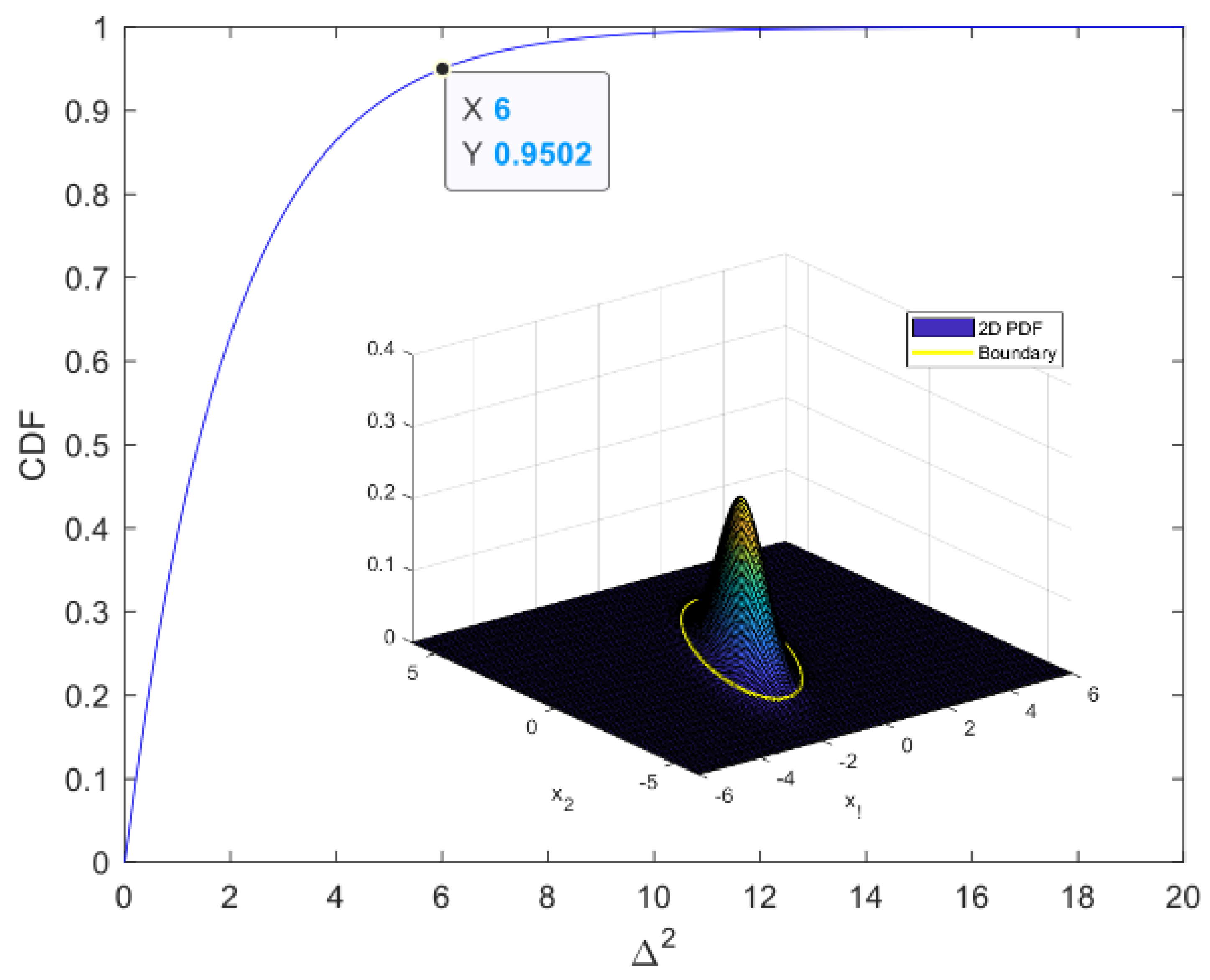
For example, to determine the boundary of 2D data $\left\{\mathbf{z}\right\}$ that follow a normal distribution with an acceptance rate of approximately 0.9502, we can determine the distance at which the cumulative distribution function of the normal distribution is 0.9502, as shown in Figure 1, and draw a contour with the same distance to obtain the boundary.

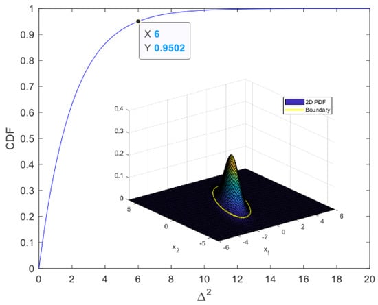
Figure 1. Cumulative distribution function of 2D normal data and boundary at acceptance rate of 0.9502. We used the squared distance ${\Delta }^2$ as the Mahalanobis distance, the details of which are provided in Section 2.2.

The obtained boundary serves as a criterion for detecting anomalies, and new data can be classified as normal if they fall within the boundary or abnormal if they fall outside the boundary.

2.2. Classification Interpretability Using the NBP

We obtain the boundary for normally distributed data, thereby being able to distinguish between normal and abnormal data based on whether they fall within or outside the boundary. If the data are classified as abnormal because they fall outside the boundary, we analyze the interpretability of classification and the changes that would be necessary for them to be classified as normal.

To ensure interpretability, we aim to solve the NBP problem by finding the boundary point closest to a datapoint $\mathbf{z}$ that falls outside the boundary. To determine the concept of nearest point, we must first define a distance, which we take to be the Mahalanobis distance. Given a probability distribution with mean $\mu$ and positive-definite covariance $\Sigma$, Mahalanobis distance ${\Delta }^2\left(\mathbf{z}\right)$ is defined as

$${\Delta }^2\left(\mathbf{z}\right)={(\mathbf{z}-\mu )}^T{\Sigma }^{-1}(\mathbf{z}-\mu ).$$

(2)

The Mahalanobis distance is an effective multivariate metric of the distance between a point (vector) and a data distribution. It is suitable for multivariate anomaly detection, classification of highly imbalanced datasets, one-class classification, and untapped use cases. In particular, when Mahalanobis distance ${\Delta }^2\left(\mathbf{z}\right)$ of point $\mathbf{z}$ from the distribution in Equation (1) is constant, the point lies on the same contour as the normal probability density function. Therefore, the boundary of normal data can be expressed as

$${\Delta }^2\left(\mathbf{z}\right)=R^2,$$

(3)

where R is a real-valued constant.

If the dataset follows normal distribution $\mathcal{N}(\mu ,\Sigma )$ and the boundary is determined by Equation (3), the optimization problem can be solved to find the NBP of $\mathbf{z}$ observed outside the boundary. Given $\mathbf{z}$, $\mu$, and $\Sigma$, we have

$$\begin{array}{ccc}& & arg\underset{\overline{z}}{min}{(\mathbf{z}-\overline{z})}^T{\Sigma }^{-1}(\mathbf{z}-\overline{z})\hfill \\ & & \mathrm{s}.\mathrm{t}.{(\overline{z}-\mu )}^T{\Sigma }^{-1}(\overline{z}-\mu )=R^2,\hfill \end{array}$$

(4)

where $\overline{z}$ denotes the NBP. To solve Equation (4), we obtain the following Laplacian:

$$\mathcal{L}(\overline{z},\lambda )={(\mathbf{z}-\overline{z})}^T{\Sigma }^{-1}(\mathbf{z}-\overline{z})-\lambda ({(\overline{z}-\mu )}^T{\Sigma }^{-1}(\overline{z}-\mu )-R^2).$$

(5)

The partial derivatives of the Laplacian are given by

$${\displaystyle \frac{\partial \mathcal{L}}{\partial \lambda }}={(\overline{z}-\mu )}^T{\Sigma }^{-1}(\overline{z}-\mu )-R^2=0,$$

(6)

$${\displaystyle \frac{\partial \mathcal{L}}{\partial \overline{z}}}=0,$$

(7)

From Equation (7), we obtain the NBP as follows:

$$\overline{z}={\displaystyle \frac{1}{1+\lambda }}\mathbf{z}+{\displaystyle \frac{\lambda }{1+\lambda }}\mu ,$$

(8)

By substituting Equation (8) into Equation (6), we obtain

$$\lambda =-1\pm \sqrt{{\displaystyle \frac{{\Delta }^2\left(\mathbf{z}\right)}{R^2}}}.$$

(9)

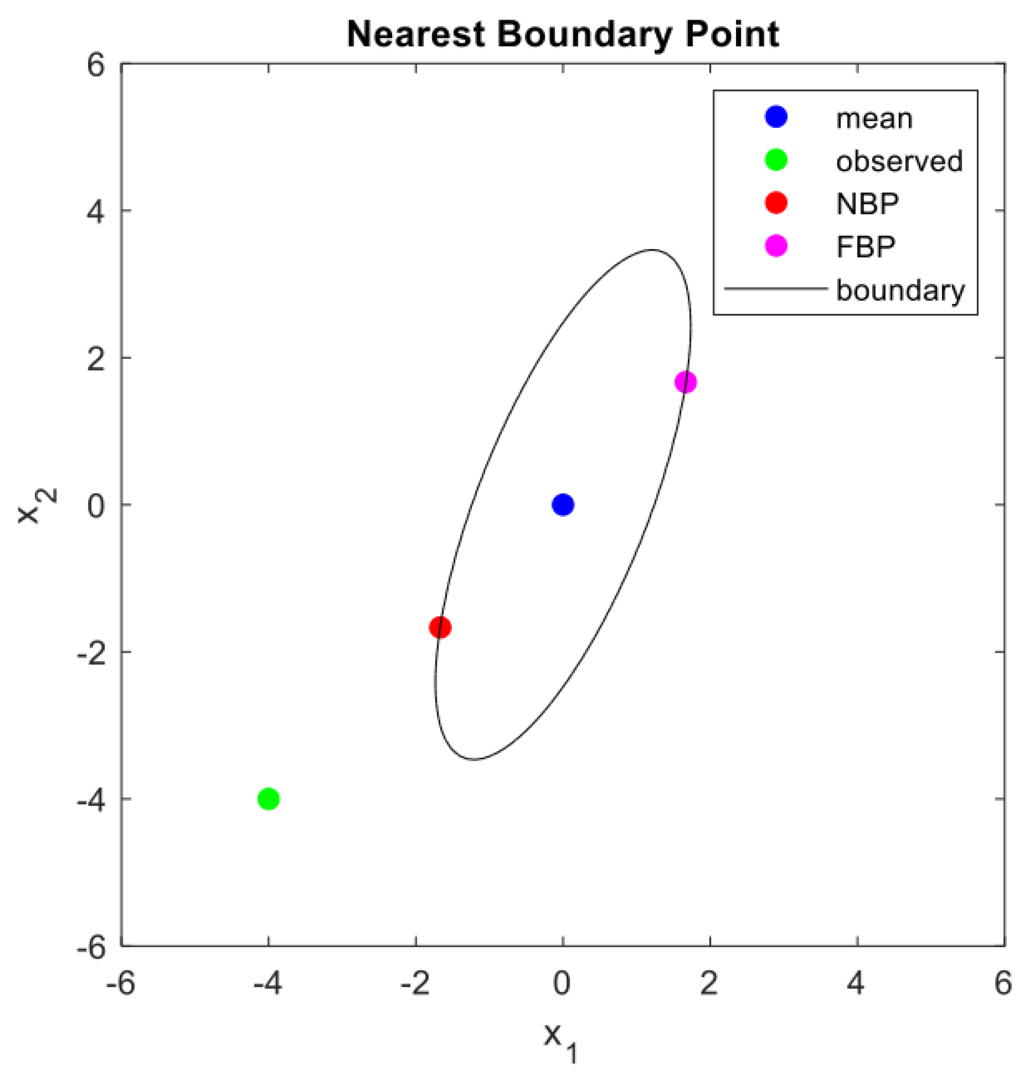
If the sign of the square root term in Equation (9) is positive, boundary point $\overline{z}$ is the nearest one, and if the sign is negative, $\overline{z}$ is the farthest boundary point, as shown in Figure 2.

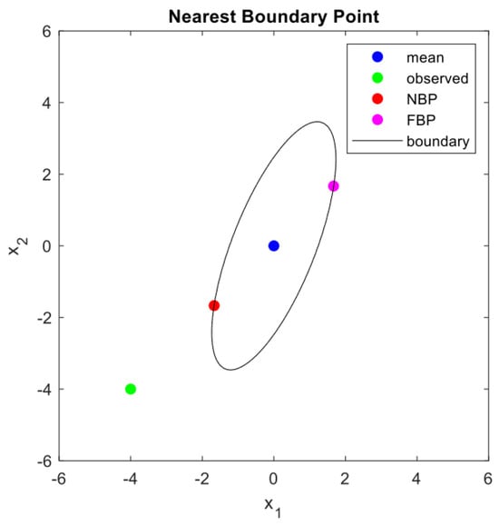
Figure 2. Solved NBP and farthest boundary point of normally distributed 2D data with boundary shown in Figure 1. The red point is the NBP of the green point, $\mathbf{z}$, which is a new observation, while the light purple point is the farthest boundary point (FBP) in terms of the Mahalanobis distance given by Equation (9).

By obtaining the NBP, $\overline{z}$, for a new observation, $\mathbf{z}$, outside the boundary, we can gain insights into interpretation, such as why $\mathbf{z}$ is outside the boundary, how far it is from the boundary, and which element values must be increased or decreased to classify it as a normal point.

2.3. Standardization of Non-Normally Distributed Data

In practice, data may not be normally distributed. To address this issue, we model data as a mixture of multiple normal distributions. When data that do not follow a normal distribution are represented as a mixture of multiple normal distributions, we can apply a normalization method.

Let $\mathbf{x}$ be a d-dimensional random variable generated by a mixture of multiple normal distributions as follows:

$$f\left(\mathbf{x}\right)=\sum _{i=1}^N{\alpha }_i\varphi \left(\mathbf{x}\right|{\mu }_i,{\Sigma }_i),$$

(10)

where ${\alpha }_i>0$, ${\sum }_{i=1}^N{\alpha }_i=1$, $\varphi (·|{\mu }_i,{\Sigma }_i)$ represents the probability density function of a d-dimensional normal distribution with mean ${\mu }_i$ and covariance ${\Sigma }_i$, and N is the number of components in the mixture. We introduce membership weight (or posterior probability) $w_i$ of class i for $\mathbf{x}$ by using Bayes’ theorem as follows:

$$w_i={\displaystyle \frac{{\alpha }_i{\varphi }_i\left(\mathbf{x}\right)}{{\sum }_{i=1}^N{\alpha }_i{\varphi }_i\left(\mathbf{x}\right)}},$$

(11)

where ${\varphi }_i\left(\mathbf{x}\right)=\varphi \left(\mathbf{x}\right|{\mu }_i,{\Sigma }_i)$. By applying the soft assignment proposed in [10], we obtain the following standardization formula:

$$\mathbf{z}=\left(\sum _{i=1}^N{w}_i{\Sigma }_i^{-1/2}\right)\left(\mathbf{x}-\sum _{i=1}^N{w}_i{\mu }_i\right),$$

(12)

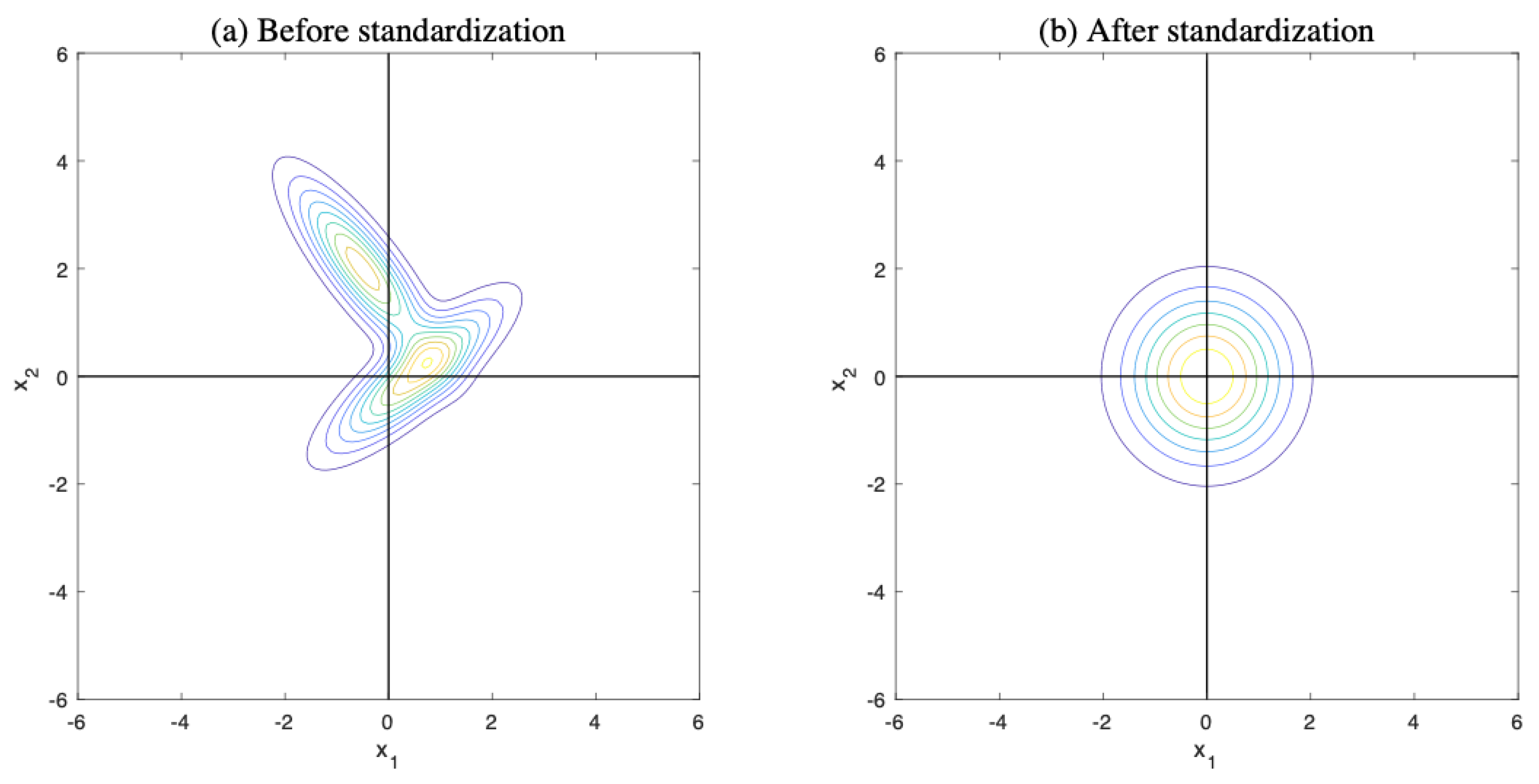
where $\mathbf{z}\backsim \mathcal{N}(0,I_d)$ is the standardized d-dimensional random vector transformed from $\mathbf{x}$ for $I_d$ being a $d\times d$ identity matrix. Figure 3 illustrates the standardization of a mixture of two normal distributions.

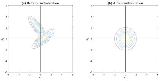
Figure 3. Standardization of mixture of multiple normal distributions. (a) Probability density function of mixture of two normal distributions with means of $(0.5,0)$ and $(-0.5,2)$ and covariances of $[1,0.7;0.7,0.7]$ and $[0.7,-0.7;-0.7,1]$. (b) Probability density function of standardized mixture.

2.4. The NBP of the One-Class SVM

The one-class SVM belongs to a family of ML algorithms known as kernel methods that use kernel functions to represent input features into a new, often higher-dimensional, space. Thus, it facilitates distinguishing between different classes, and the resulting decision boundary is often simpler and more interpretable than that in the original feature space. This approach avoids the need for explicit feature transformations, which can be computationally expensive, and is often referred to as the kernel trick.

A Gaussian kernel is commonly used to perform the kernel trick and is universal, meaning that it can uniformly approximate any arbitrary continuous target function. Gaussian kernels offer a valuable advantage by transferring data from the original plane into a hyperplane for analysis. This capability can resolve a significant limitation of the Mahalanobis distance which is known to perform inadequately for datasets characterized by linearity and heteroscedasticity. By utilizing Gaussian kernels, the shortcomings associated with Mahalanobis distance in these contexts can be effectively mitigated.

After training, the decision function of the SVM for observation $\mathbf{x}$ can be obtained as follows:

$$g\left(\mathbf{x}\right)=\sum _{i=1}^N{\beta }_i\phi \left(\mathbf{x}\right|{\mathbf{x}}_i,\sigma )-b,$$

(13)

where ${\mathbf{x}}_i$ denotes the i-th support vector, b is the bias term, N is the number of support vectors, and $\phi \left(\mathbf{a}\right|\mathbf{b},\sigma )$ is a Gaussian kernel with width $\sigma$ and given by

$$\phi \left(\mathbf{a}\right|\mathbf{b},\sigma )=exp\left\{-{\displaystyle \frac{{(\mathbf{a}-\mathbf{b})}^T(\mathbf{a}-\mathbf{b})}{2{\sigma }^2}}\right\}.$$

(14)

Because the decision function in Equation (13) is a linear sum of Gaussian functions, we have the following relationship between $g\left(\mathbf{x}\right)$ in Equation (13) and $f\left(\mathbf{x}\right)$ in Equation (10):

$$\begin{array}{ccc}\hfill g\left(\mathbf{x}\right)& =& \sum _{i=1}^N{\beta }_{i}exp\left\{-{\displaystyle \frac{{(\mathbf{x}-{\mathbf{x}}_i)}^T(\mathbf{x}-{\mathbf{x}}_i)}{2{\sigma }^2}}\right\}-b,\hfill \\ \hfill K\left(g\right(\mathbf{x})+b)& =& \sum _{i=1}^N{\alpha }_i\varphi \left(\mathbf{x}\right|{\mu }_i,{\Sigma }_i),\hfill \\ & =& f\left(\mathbf{x}\right)\hfill \end{array}$$

(15)

where ${K=\{\left(2\pi \right)}^{d/2}{|\Sigma |}^{1/2}{\sum }_{i=1}^N{\beta }_i{\}}^{-1}$, ${\alpha }_i={\displaystyle \frac{{\beta }_i}{{\sum }_{i=1}^N{\beta }_i}}$, ${\Sigma }_i={\sigma }^2{I}_d$, and ${\mu }_i={\mathbf{x}}_i$ for all $i=1,\dots ,N$.

As shown in Equation (15), $K\left(g\right(\mathbf{x})+b)$ takes the form of multiple mixtures with normal distributions. As K and b are constants, we can transform the distribution of an $\mathbf{x}$ space into a standardized normal distribution of another $\mathbf{z}$ space using Equations (11) and (12). The posterior probability can be derived as

$$w_i={\displaystyle \frac{{\beta }_i\phi \left(\mathbf{x}\right|{\mathbf{x}}_i,\sigma )}{{\sum }_{i=1}^N{\beta }_i\phi \left(\mathbf{x}\right|{\mathbf{x}}_i,\sigma )}}={\displaystyle \frac{{\beta }_i\phi \left(\mathbf{x}\right|{\mathbf{x}}_i,\sigma )}{g\left(\mathbf{x}\right)+b}}.$$

(16)

As ${\sum }_{i=1}^N{w}_i=1$ and ${\Sigma }_i=\sigma I_d$, we have

$$\mathbf{z}={\displaystyle \frac{1}{\sigma }}\left(\mathbf{x}-\sum _{i=1}^N{w}_i{\mathbf{x}}_i\right).$$

(17)

As $\mathbf{z}$ follows a normal distribution, that is, $\mathbf{z}\sim \mathcal{N}(0,I_d)$, we obtain $\lambda$ from Equation (9) as follows:

$$\lambda =\sqrt{{\displaystyle \frac{{\mathbf{z}}^T\mathbf{z}}{R^2}}}-1.$$

(18)

By numerically computing ${\mathbf{x}}_b=arg{min}_{\mathbf{x}}{g}^2\left(\mathbf{x}\right)$ from training data, we calculate ${\mathbf{z}}_b$ using Equation (17) and derive the Mahalanobis distance of the boundary as $R^2={\mathbf{z}}_b^T{\mathbf{z}}_b$. Substituting $\lambda$ into Equation (8), we obtain the following NBP in the $\mathbf{z}$ space:

$$\overline{z}=\sqrt{{\displaystyle \frac{{\mathbf{z}}_b^T{\mathbf{z}}_b}{{\mathbf{z}}^T\mathbf{z}}}}\mathbf{z},$$

(19)

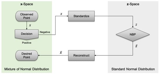
and reconstructing $\overline{z}$ into the $\mathbf{x}$ space, we obtain the NBP of the new observation, $\mathbf{x}$.

$$\overline{x}=\sigma \overline{z}+\sum _{i=1}^N{\overline{w}}_i{\mathbf{x}}_i.$$

(20)

As ${\overline{w}}_i$ cannot be computed explicitly, we use $w_i$ instead of ${\overline{w}}_i$ and calculate Equation (17) by letting $\mathbf{x}=\overline{x}$ and applying Equations (19) and (20) repeatedly until $\overline{x}$ converges.

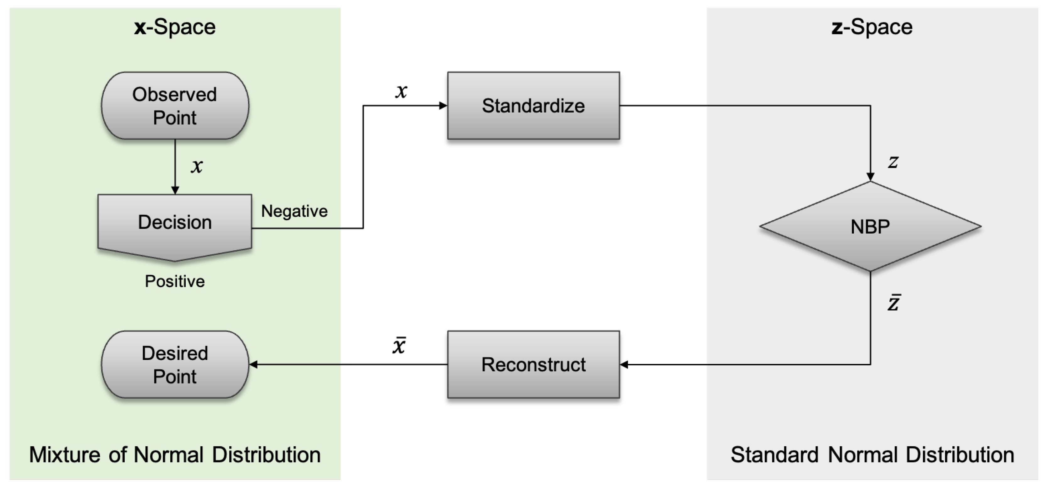
Figure 4 illustrates the proposed process for determining the desired point (that is, NBP) from the SVM decision function.

Figure 4. Block diagram for finding the desired point (or the NBP) $\overline{x}$ when a new observation $\mathbf{x}$ is classified as negative. Each standardized $\mathbf{z}$, NBP $\overline{z}$, and reconstructed point $\overline{x}$ can be computed by Equations (17), (19) and (20), respectively.

3. Simulation Results

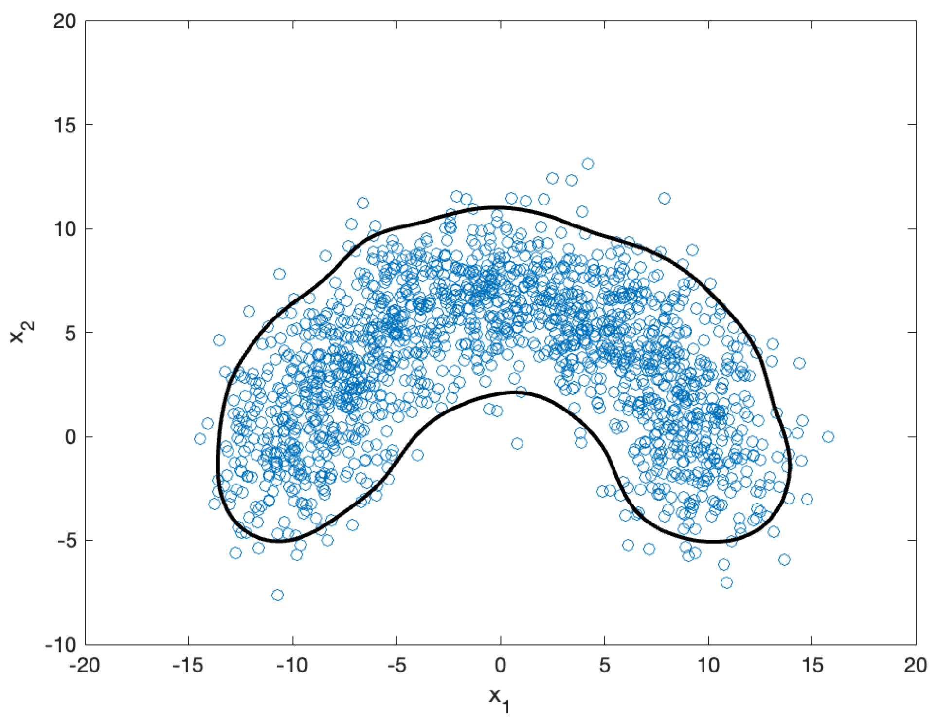
This section presents simulation results used to validate the proposed method for solving the NBP in the one-class SVM. The results are reported stepwise, and the final outcomes are provided. For the simulation, we used 2D nonlinear data. As shown in Figure 5, we randomly sampled 1571 datapoints (blue circles) from a normal distribution with mean ${[10cos\theta ,10sin\theta ]}^T$ and covariance $2^2{I}_2$, where $\theta \in (0,\pi )$ and $I_2$ is a 2D identity matrix. We then applied the one-class SVM to extract a region bounded by a decision function (black contour in the figure).

Figure 5. Randomly sampled (1571) datapoints (blue circles) and their one-class SVM boundary (black contour). The boundary effectively encloses the majority of the datapoints, excluding a few outliers, demonstrating a smooth and robust classification performance that is less sensitive to noise.

Figure 6 shows the standardized datapoints (red circles) and the boundary in the $\mathbf{z}$ space, which correspond to the original datapoints in the $\mathbf{x}$ space in Figure 5. After transformation, the data were normally distributed and centered at the origin of the $\mathbf{z}$ plane. To quantitatively evaluate the effectiveness of the standardization in Figure 6, we performed a Kolmogorov–Smirnov test [11] on the 2D data. The results confirmed the normality of the standardized datapoints, with a significance level of $p<0.00$.

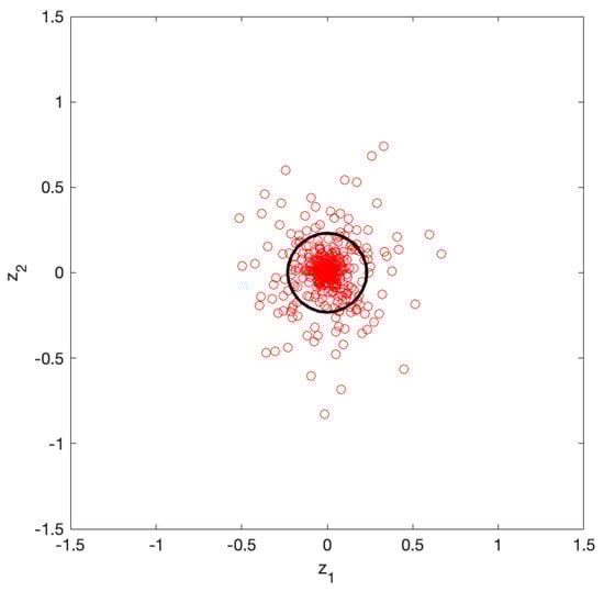
Figure 6. Standardized datapoints (red circles) and their boundary (black contour) in the $\mathbf{z}$ space. The boundary effectively encloses the majority of the datapoints while excluding outliers, similar to the original space. In the 2D standardized space, the boundary appears geometrically circular.

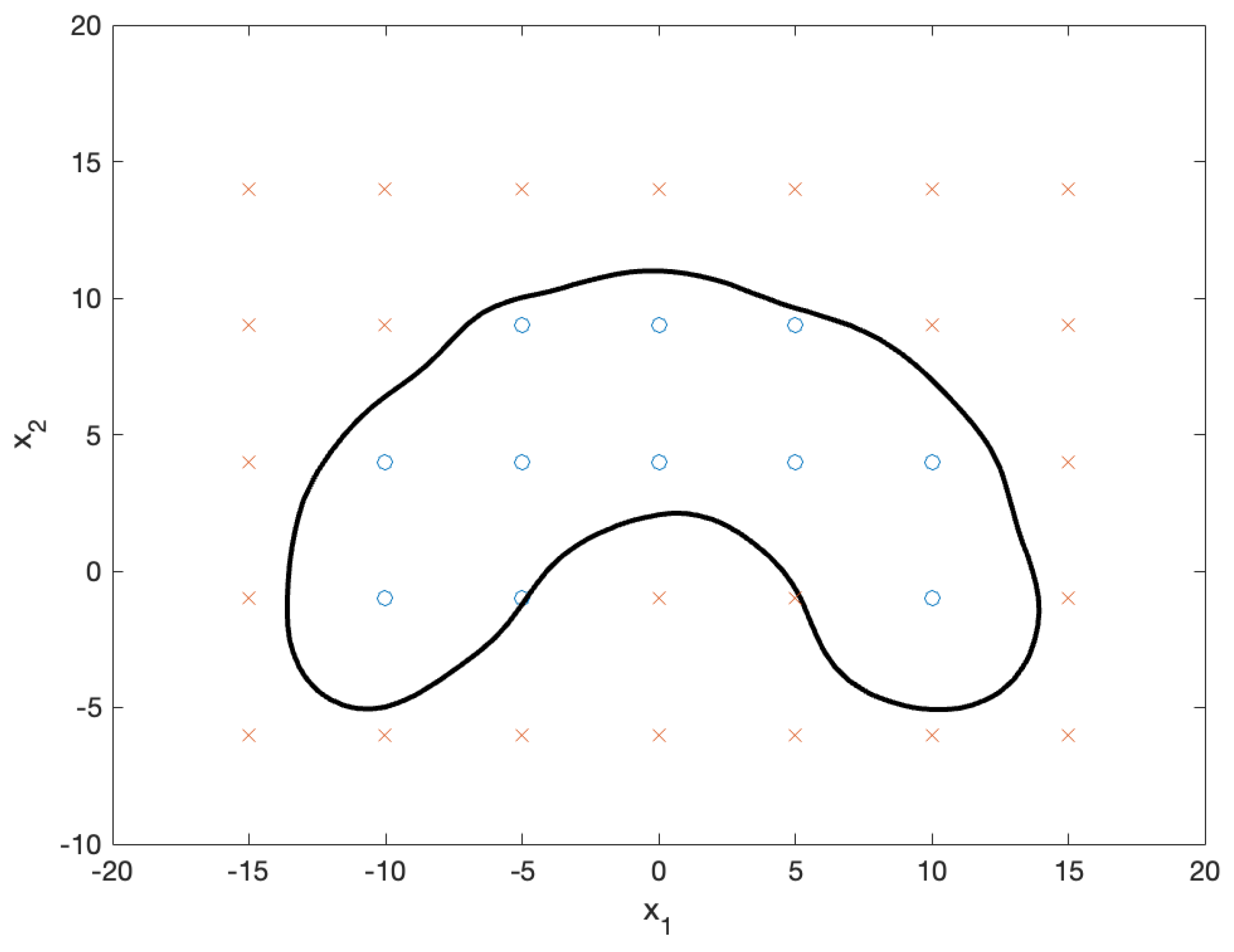
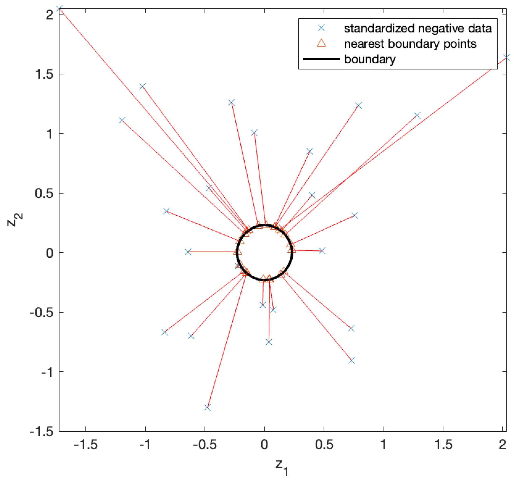
The decision function for the SVM was obtained through training. Figure 7 shows the test data used to evaluate the decision function. A positive classification was assigned to the test data that fell within the decision boundary, whereas a negative classification was assigned to the test data outside the boundary. As we focused on negative samples, we solved the NBP problem for negative test samples. First, we standardized the negative test samples and computed their NBPs, as shown in Figure 8. The x marks in the figure represent the standardized negative test samples, and the triangular marks represent their NBPs. The NBPs lie on the black contour, which represents the decision boundary.

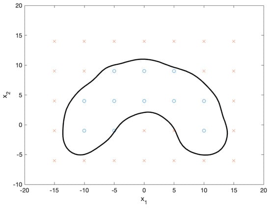
Figure 7. Decision boundary (black contour) that separates positive samples (blue circles) from negative samples (red circles). The boundary effectively distinguishes between the two classes, even for datapoints near the decision boundary.

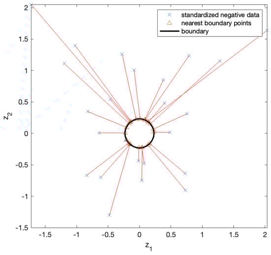
Figure 8. Standardized negative test points (x marks) and their NBPs (triangular marks). The NBPs lie on the decision boundary (black contour) and are accurately identified in the direction toward the center of the circular boundary.

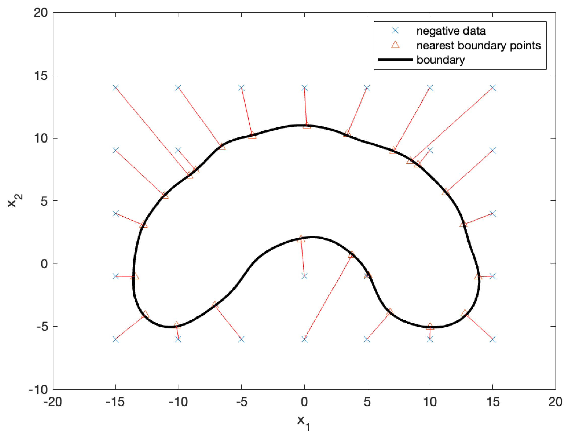
By mapping the datapoints and the NBPs from the $\mathbf{z}$ plane, as shown in Figure 8, onto the $\mathbf{x}$ plane, we obtained the final solution (that is, the desired points), as illustrated in Figure 9. The x marks in the figure represent negative test samples, whereas the triangular marks represent their NBPs. The NBPs lie on the black contour, which represents the decision boundary.

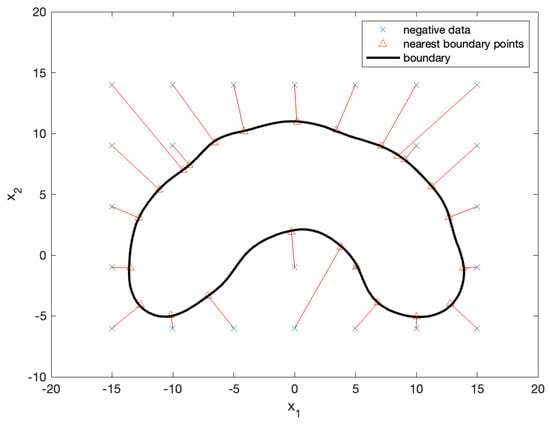
Figure 9. Negative test samples (x marks) and their NBPs (triangular marks). The NBPs lie on the decision boundary (black contour). The results show that the nearest boundary points identified in the $\mathbf{x}$ plane are consistently mapped back to the $\mathbf{x}$ plane, effectively locating the nearest points on the decision boundary.

4. Applications

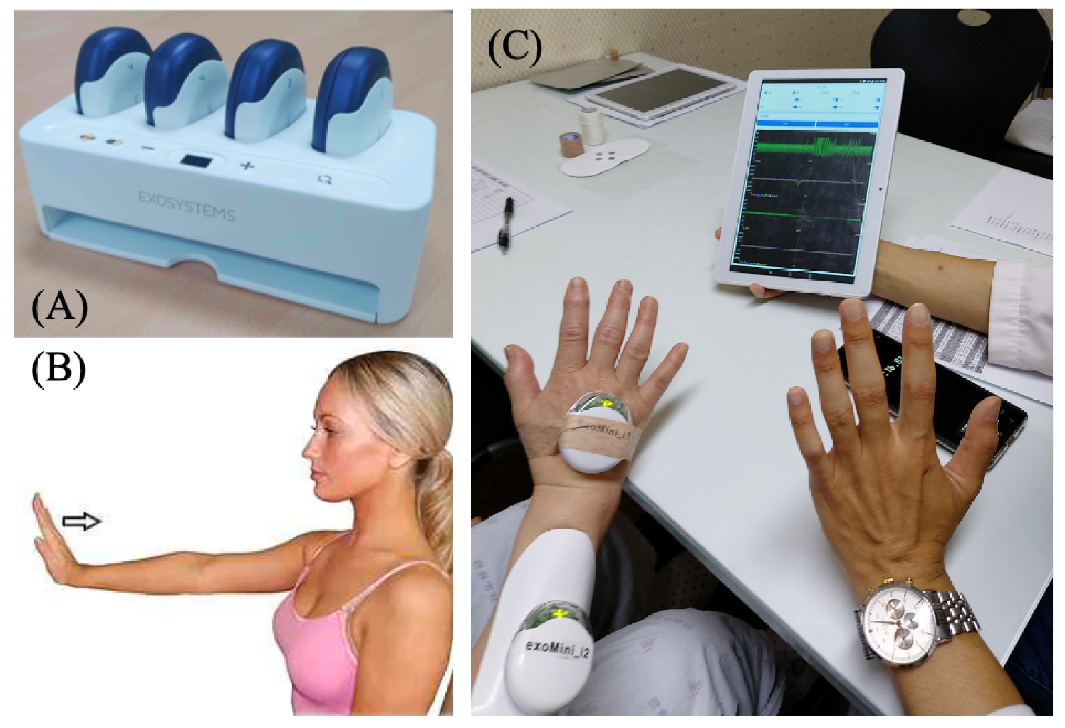
We present a practical application of the proposed interpretable SVM to rehabilitation assessment along with experimental results obtained from analysis and testing. Our aims were to evaluate the forearm muscle function of patients undergoing rehabilitation through measurements of surface electromyography (sEMG) and an inertial measurement unit (IMU) as well as to determine appropriate countermeasures for functional electric stimulation (FES) and physical therapy using a robot. Specifically, we employed the exoPill sensor [12], which is a modular device developed by ExoSystems Inc. (Gyeonggi-do, Republic of Korea). It integrates sEMG electrodes and an IMU, as depicted in Figure 10A. We considered wrist extension as the evaluated rehabilitation movement, as illustrated in Figure 10B, by attaching the sEMG electrodes to the extensor carpi radialis muscles and the IMU to the back of the hand, as shown in Figure 10C.

Figure 10. (A) exoPill measurement system developed by ExoSystems. (B) Wrist extension for evaluation. (C) Experimental setup.

We recruited 40 participants for our study, including 20 healthy individuals and 20 patients who recovered from stroke. Each participant wore a measuring device and alternated resting and wrist extensions 10 times at 5 s intervals. For the stroke patients, the measuring device was worn on the side affected by hemiplegia, and an upper-extremity Fugl–Meyer assessment (FMA) was conducted by a clinical staff member. The maximum score for the FMA was 14.

From the sEMG signal, features such as power (PWR), median frequency (MDF), mean frequency (MNF), and root mean square (RMS) were extracted. From the IMU signal, the velocity (VEL) and range of movement (ROM) were extracted. Using these features from normal individuals as positive samples, we trained the one-class SVM and obtained a decision function by fine-tuning. To improve the training results, we performed data augmentation through a boosting technique.

The one-class SVM decision function trained using the features extracted from normal individuals was applied to the features of stroke patients to classify the muscle function of each patient. For patients classified as abnormal, the NBP was solved to analyze the causes of such classification and possible countermeasures for improving rehabilitation. This process was performed considering the 14 patients whose data were excluded owing to sensor signal omission or mismeasurement.

The evaluation results are listed in Table 1. Out of the 14 patients, 10 were classified as abnormal. For each of these 10 patients, we analyzed the differences between the measurements and NBPs per feature.

Table 1. Subtraction of NBPs and negative test samples.

No.	PWR	MDF	MNF	RMS	VEL	ROM
2	0.0216	${\mathbf{28.6384}}^{†}$	2.1470	${\mathbf{2.7642}}^{†}$	6.2059	0.3870
3	${\mathbf{0.0891}}^{†}$	${\mathbf{20.4617}}^{†}$	4.1815	1.1141	−6.8674	0.1913
4	${\mathbf{0.0746}}^{†}$	${\mathbf{27.4724}}^{†}$	−3.1780	${\mathbf{2.2990}}^{†}$	0.1551	0.2810
6	${\mathbf{0.0788}}^{†}$	${\mathbf{47.4210}}^{†}$	${\mathbf{24.4754}}^{†}$	${\mathbf{2.6820}}^{†}$	${\mathbf{23.0072}}^{†}$	${\mathbf{1.0584}}^{†}$
7	${\mathbf{0.0694}}^{†}$	${\mathbf{35.6850}}^{†}$	−7.1576	${\mathbf{2.4398}}^{†}$	0.8068	0.2192
8	$-{\mathbf{0.0726}}^{†}$	−0.3492	1.3856	$-{\mathbf{4.0477}}^{†}$	5.4616	0.2313
10	${\mathbf{0.1037}}^{†}$	${\mathbf{56.0339}}^{†}$	9.5026	${\mathbf{3.7628}}^{†}$	${\mathbf{18.7112}}^{†}$	${\mathbf{1.2062}}^{†}$
11	0.0496	${\mathbf{38.2881}}^{†}$	${\mathbf{35.0693}}^{†}$	0.4746	${\mathbf{18.8491}}^{†}$	0.3364
17	−0.0014	−0.8882	−2.4736	−0.4333	5.4364	0.0162
18	${\mathbf{0.0883}}^{†}$	${\mathbf{28.7705}}^{†}$	2.2433	−0.1190	${\mathbf{15.5825}}^{†}$	${\mathbf{0.8308}}^{†}$
$\sigma$	0.0216	6.3266	4.0456	0.4805	4.0995	0.1378

† When the difference between the NBP and corresponding feature of the negative test sample was larger than 3$\sigma$, we identified the feature as the main factor, where $\sigma$ denotes the standard deviation of each feature from the value for normal individuals.

A higher difference indicated that more effort was required for patients to be classified as normal. To identify the main factors contributing to patient’s abnormalities, we used the standard deviation of the measurements from normal individuals. The corresponding results are listed in Table 2, where + and − indicate normal and abnormal, respectively.

Table 2. Results of muscle function assessment.

No.	FMA	SVM	Main Factors from NBP
2	12	−	MDF, RMS
3	9	−	PWR, MDF
4	12	−	PWR, MDF, RMS
6	0	−	PWR, MDF, MNF, RMS, VEL, ROM
7	12	−	PWR, MDF, RMS
8	12	−	PWR, RMS
10	1	−	PWR, MDF, RMS, VEL, ROM
11	1	−	MDF, MNF, VEL
12	14	+
15	14	+
16	14	+
17	12	−	None
18	6	−	PWR, MDF, VEL, ROM
20	14	+

By applying the interpretable SVM proposed in this paper, it is possible to classify the muscle function of patients as either normal or abnormal based on sEMG and IMU measurements. In cases where the function is classified as abnormal, the method can identify the main factors responsible for the abnormality. Depending on these factors, such as whether the abnormal muscle function is due to issues with muscle recruitment or physical problems like muscle contractures, appropriate treatments can be prescribed. These treatments may include FES for muscle recruitment issues, or robotics approach (e.g., exoskeleton) for physical problems.

As indicated in Table 2, the SVM decision function classified patients with FMA scores of 14 (that is, the highest score) as normal and those with lower scores as abnormal. In the abnormal group, the main abnormality factors were identified by solving the NBP problem, and different factors were identified per patient. Once the main abnormality factors for each patient were determined, PWR, MDF, MNF, and RMS derived from sEMG signals were used to define countermeasures for FES treatment. On the other hand, VEL and ROM provided guidelines for using robotic therapy as physical assistance. For example, for patient 3, PWR and MDF were the main abnormal factors, indicating the need for physical therapy using FES to address muscle recruitment issues. Patients 6, 10, 11, and 18 required FES treatment and additional physical therapy using robotic assistance to address movement dynamic issues.

5. Conclusions

We propose an interpretable SVM that enables the derivation of the causes of data classified as abnormal by one-class classification and the analysis of countermeasures for rehabilitation. The proposed method is based on the Mahalanobis distance and involves obtaining the NBP of abnormal data. The NBP indicates the shortest path from the abnormal data to the normal boundary and allows to identify features that contribute to anomaly along with their contribution extent.

The proposed method for obtaining the NBP of abnormal data involves standardizing the SVM decision function. Given that this function with a Gaussian kernel can be expressed as a mixture of normal distributions in the $\mathbf{x}$ space, we can approximate the decision function to a normal distribution in the $\mathbf{z}$ space. After standardization, we obtain the NBP in the $\mathbf{z}$ space and reconstruct it back to the $\mathbf{x}$ space.

We used a 2D nonlinear dataset to simulate and test the proposed method, validating its feasibility and applicability through simulations. Moreover, we applied the proposed method to rehabilitation. Using sEMG and IMU measurements, we classified the status of the patient’s muscle function and analyzed the underlying causes of anomalies and possible therapeutic countermeasures.

References

- Giger, M.L. Machine learning in medical imaging. J. Am. Coll. Radiol. 2018, 15, 512–520. [Google Scholar] [CrossRef] [PubMed]
- Currie, G.; Hawk, K.E.; Rohren, E.; Vial, A.; Klein, R. Machine learning and deep learning in medical imaging: Intelligent imaging. J. Med. Imaging Radiat. Sci. 2019, 50, 477–487. [Google Scholar] [CrossRef] [PubMed]
- Massaro, A.; Ricci, G.; Selicato, S.; Raminelli, S.; Galiano, A. Decisional support system with artificial intelligence oriented on health prediction using a wearable device and big data. In Proceedings of the 2020 IEEE International Workshop on Metrology for Industry 4.0 and IoT, Roma, Italy, 3–5 June 2020; pp. 718–723. [Google Scholar]
- Chawala, N.; Bowyer, K.; Hall, L.; Kegelmeyer, W. SMOTE: Synthetic Minority Over-sampling Technique. J. Artif. Intell. Res. 2002, 16, 321–357. [Google Scholar] [CrossRef]
- Liu, L.; Wu, X.; Li, S.; Li, Y.; Tan, S.; Bai, Y. Solving the class imbalance problem using ensemble algorithm: Application of screening for aortic dissection. BMC Med. Inform. Decis. Mak. 2022, 22, 82. [Google Scholar] [CrossRef] [PubMed]
- Xuan, L.; Zhigang, C.; Fan, Y. Exploring of clustering algorithm on class-imbalanced data. In Proceedings of the 8th International Conference on Computer Science and Education, Colombo, Sri Lanka, 26–28 April 2013. [Google Scholar]
- Liu, Y.-H.; Huang, H.-P. Towards a high-stability EMG recognition system for prosthesis control: A one-class classification based non-target EMG pattern filtering scheme. In Proceedings of the 2009 IEEE International Conference on Systems, Man and Cybernetics, San Antonio, TX, USA, 11–14 October 2009; pp. 4752–4757. [Google Scholar]
- Faula, Y.; Eglin, V.; Bres, S. One-class detection and classification of defects on concrete surfaces. In Proceedings of the 2021 IEEE International Conference on Systems, Man, and Cybernetics, Melbourne, Australia, 17–20 October 2021; pp. 826–831. [Google Scholar]
- Schölkopf, B.; Williamson, R.C.; Smola, A.; Shawe-Taylor, J.; Platt, J. Support vector method for novelty detection. Adv. Neural Inf. Process. Syst. 1999, 12, 582–588. [Google Scholar]
- Li, M.; Schwartzman, A. Standardization of multivariate Gaussian mixture models and background adjustment of PET images in brain oncology. Ann. Appl. Stat. 2018, 12, 2197–2227. [Google Scholar] [CrossRef]
- Marsaglia, G.; Tsang, W.; Wang, J. Evaluating Kolmogorov’s Distribution. J. Stat. Softw. 2003, 8, 1–4. [Google Scholar] [CrossRef]
- exoPill: AI-Based Wearable Healthcare Solution. Available online: https://www.exosystems.io/exopill?lang=en (accessed on 1 August 2023).
Disclaimer/Publisher’s Note: The statements, opinions and data contained in all publications are solely those of the individual author(s) and contributor(s) and not of MDPI and/or the editor(s). MDPI and/or the editor(s) disclaim responsibility for any injury to people or property resulting from any ideas, methods, instructions or products referred to in the content. |
© 2024 by the authors. Licensee MDPI, Basel, Switzerland. This article is an open access article distributed under the terms and conditions of the Creative Commons Attribution (CC BY) license (https://creativecommons.org/licenses/by/4.0/).