Abstract
The early detection of breast cancer is essential for improving treatment outcomes, and recent advancements in artificial intelligence (AI), combined with image processing techniques, have shown great potential in enhancing diagnostic accuracy. This study explores the effects of various image processing methods and AI models on the performance of early breast cancer diagnostic systems. By focusing on techniques such as Wiener filtering and total variation filtering, we aim to improve image quality and diagnostic precision. The novelty of this study lies in the comprehensive evaluation of these techniques across multiple medical imaging datasets, including a DCE-MRI dataset for breast-tumor image segmentation and classification (BreastDM) and the Breast Ultrasound Image (BUSI), Mammographic Image Analysis Society (MIAS), Breast Cancer Histopathological Image (BreakHis), and Digital Database for Screening Mammography (DDSM) datasets. The integration of advanced AI models, such as the vision transformer (ViT) and the U-KAN model—a U-Net structure combined with Kolmogorov–Arnold Networks (KANs)—is another key aspect, offering new insights into the efficacy of these approaches in different imaging contexts. Experiments revealed that Wiener filtering significantly improved image quality, achieving a peak signal-to-noise ratio (PSNR) of 23.06 dB and a structural similarity index measure (SSIM) of 0.79 using the BreastDM dataset and a PSNR of 20.09 dB with an SSIM of 0.35 using the BUSI dataset. When combined filtering techniques were applied, the results varied, with the MIAS dataset showing a decrease in SSIM and an increase in the mean squared error (MSE), while the BUSI dataset exhibited enhanced perceptual quality and structural preservation. The vision transformer (ViT) framework excelled in processing complex image data, particularly with the BreastDM and BUSI datasets. Notably, the Wiener filter using the BreastDM dataset resulted in an accuracy of 96.9% and a recall of 96.7%, while the combined filtering approach further enhanced these metrics to 99.3% accuracy and 98.3% recall. In the BUSI dataset, the Wiener filter achieved an accuracy of 98.0% and a specificity of 98.5%. Additionally, the U-KAN model demonstrated superior performance in breast cancer lesion segmentation, outperforming traditional models like U-Net and U-Net++ across datasets, with an accuracy of 93.3% and a sensitivity of 97.4% in the BUSI dataset. These findings highlight the importance of dataset-specific preprocessing techniques and the potential of advanced AI models like ViT and U-KAN to significantly improve the accuracy of early breast cancer diagnostics.
1. Introduction
The literature on breast cancer detection and diagnosis using image processing and artificial intelligence (AI) reveals significant advancements and varied methodologies, reflecting the ongoing evolution in this critical field. Central to these advancements is the integration of AI techniques, such as machine learning (ML) and deep learning (DL), which have significantly enhanced the accuracy and efficiency of breast cancer detection.
The article [1] systematically reviews the application of image processing in breast cancer recognition, detailing advancements in detection, segmentation, registration, and fusion techniques. The authors emphasize the promising future of unsupervised and transfer learning in enhancing diagnostic accuracy and patient privacy protection. Similarly, Zerouaou and Idri [2] conducted a structured literature review, identifying deep learning as the predominant method for classification tasks in breast cancer imaging, with mammograms being the most extensively studied imaging modality. They highlight the importance of image preprocessing, feature extraction, and public datasets in improving diagnostic performance.
The early and accurate detection of breast cancer remains a critical challenge in medical diagnostics, with significant implications for patient outcomes. Advances in medical imaging and artificial intelligence (AI) have opened new avenues for enhancing the precision of tumor detection, particularly in mammographic imaging. SA Khan et al. [3] conducted a comprehensive survey of medical imaging fusion techniques, emphasizing the strengths and limitations of various methods in improving diagnostic accuracy. Their work highlights key challenges, such as noise sensitivity, computational complexity, and the difficulty of preserving essential image details, which continue to impede the broader application of these techniques in clinical practice. Addressing these challenges is vital in developing more reliable and effective fusion methods for medical imaging.
Building on this foundation, SU Khan et al. [4] explored the application of deep learning models for semantic segmentation in breast tumor detection. Through a comparative analysis, they identified the Dilation 10 (global) model as particularly effective, achieving high pixel accuracy in differentiating tumor regions in mammograms. However, their study also uncovered significant challenges, including dataset imbalance and the risk of over-segmentation, which can lead to false positives. These findings underscore the need for careful model selection, balanced datasets, and further refinement of AI-based methods to enhance the reliability and accuracy of early breast cancer detection.
Expert human knowledge is essential in traditional cancer image recognition paradigms. The process involves image segmentation, feature extraction, and the application of machine learning algorithms to these handcrafted features in order to develop predictive models. In contrast, deep learning offers an end-to-end solution that processes raw images directly. Deep learning systems use biologically inspired neural networks to transform data through multiple nonlinear layers, yielding progressively more abstract representations. This hierarchical approach enables the formation of complex, highly discriminative models, significantly enhancing the ability to classify cancerous images accurately. These studies underscore the pivotal role of advanced image processing and AI technologies in enhancing the early detection, diagnosis, and treatment of breast cancer. Integrating these technologies improves diagnostic accuracy and efficiency and holds promise for personalized medicine, ultimately aiming to improve patient outcomes and reduce mortality rates associated with breast cancer.
Despite significant advancements in the application of artificial intelligence (AI) and image processing techniques for breast cancer detection, several critical challenges remain unresolved. The current body of literature extensively documents the efficacy of machine learning (ML) and deep learning (DL) models, which have markedly improved the accuracy of breast cancer diagnostics. However, a persistent gap exists concerning the generalizability and robustness of these models when applied across a diverse range of medical imaging modalities. A predominant limitation within the existing research is the heavy reliance on single-modality datasets. This dependency constrains the performance of AI models, particularly when these models are deployed across various imaging modalities, such as mammography, ultrasound, magnetic resonance imaging (MRI), and histopathology [5,6]. The heterogeneity in image quality and the presence of modality-specific noise further exacerbate this issue, leading to variability in diagnostic outcomes and diminishing the models’ efficacy in clinical settings. In response to these identified gaps, the present study undertakes a systematic exploration of the integration of advanced image processing techniques with state-of-the-art AI models. The primary objective is to enhance diagnostic performance across multiple medical imaging modalities. To this end, the study focuses on the application of Wiener filtering and total variation filtering as preprocessing steps to refine image quality. These preprocessing techniques are then evaluated in conjunction with cutting-edge AI models, specifically the vision transformer (ViT) and the U-KAN model.
Breast cancer remains one of the most significant health challenges worldwide, demanding continual improvements in diagnostic accuracy and early detection. This study investigates the impact of various image processing techniques, notably Wiener filtering and total variation filtering, on the quality and diagnostic precision of breast cancer detection across different medical imaging modalities. Additionally, it evaluates the consistency and robustness of advanced AI models, such as vision transformers (ViTs) and U-KAN, when applied to diverse datasets, including dynamic contrast-enhanced MRI (DCE-MRI), ultrasound, mammography, and histopathology. By addressing these research questions, this study fills a critical gap in the literature, providing a comprehensive evaluation of AI models in conjunction with tailored image preprocessing techniques. The findings aim to contribute to developing more robust, generalizable, and clinically applicable diagnostic systems for early breast cancer detection.
The remainder of this paper is organized as follows. Section 2 reviews related work on preprocessing techniques and AI-driven breast cancer detection and segmentation. The methodology, including image processing and ViT model training, is detailed in Section 3. Section 4 presents the validation of the theoretical framework through experimental studies. Concluding remarks are provided in Section 5.
2. Related Works
This section provides a comprehensive overview of the key components of our research, which focuses on medical image preprocessing, breast cancer detection, lesion segmentation, and the selection of appropriate AI models for training. The section begins by establishing the necessity of each technological implementation, highlighting the critical role that preprocessing plays in standardizing medical images and enhancing diagnostic accuracy. Following this, it delves into the methodologies used for breast cancer detection, emphasizing the importance of accurate image segmentation in localizing lesions. The discussion extends to the selection and training of suitable AI models, underscoring the criteria and rationale for their use in achieving optimal performance. Additionally, the chapter reviews recent advancements in each of these areas, analyzing the effectiveness of contemporary techniques and the persistent challenges they aim to address. Through a rigorous examination of these elements, the chapter aims to contextualize our approach within the broader landscape of medical imaging and AI, demonstrating the integrated strategy employed to improve early breast cancer detection and diagnosis.
2.1. Preprocessing
Preprocessing is a crucial step in medical imaging, enhancing the quality and consistency of input data, regardless of its source. Through the application of standardized preprocessing techniques, such as noise reduction, contrast enhancement, and normalization, the variability inherent in images from different sources can be minimized. This standardization is vital for improving the robustness and generalizability of AI models, as it allows them to focus on diagnostically relevant features, rather than extraneous variations introduced via differing imaging conditions or equipment. Kumar and Nachamai [7] underscore the importance of these techniques, demonstrating that filters like the Wiener filter effectively mitigate common noise types, such as Gaussian and speckle, prevalent in medical images. This not only enhances image clarity but also ensures that the images meet a consistent quality standard, which is essential for accurate classification and segmentation, ultimately supporting the reliable performance of AI models in medical diagnostics.
Fan et al. [8] explore the progression of image denoising techniques, from classical approaches to deep learning-based methods, and underscore the distinct strengths of each. Spatial filters, such as Wiener filtering, are shown to effectively reduce noise while preserving a balance between noise suppression and detail retention, which is demonstrated in Figure 1. The figure also illustrates that collaborative filtering techniques like BM3D excel in maintaining edges while reducing noise. In Figure 2, the performance of total variation (TV) regularization is highlighted, showcasing its capability to preserve edges and structural details, though it may occasionally introduce minor texture artifacts. This figure also compares the outcomes of non-local means (NLM) and low-rank-based methods, illustrating their strengths in handling noise across various image structures. These visual comparisons elucidate the differential performance of various denoising techniques, thereby reinforcing the rationale for selecting methods tailored to specific image properties and noise characteristics.
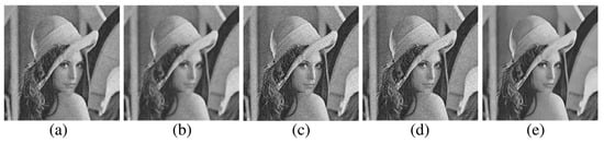
Figure 1.
Visual comparison of denoising methods using the Lena image with Gaussian noise (): (a) Wiener filter (PSNR: 27.81; SSIM: 0.707); (b) bilateral filter (PSNR: 27.88; SSIM: 0.712); (c) PCA (PSNR: 26.68; SSIM: 0.596); (d) wavelet transform (PSNR: 21.74; SSIM: 0.316); (e) BM3D (PSNR: 31.26; SSIM: 0.845) [8].
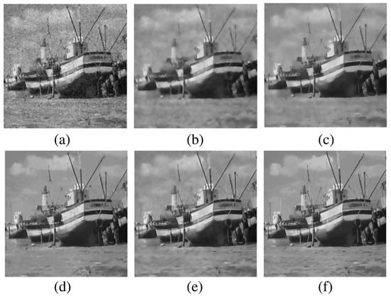
Figure 2.
Visual comparison of denoising methods on the Boat image with Gaussian noise (): (a) TV regularization (PSNR: 22.95; SSIM: 0.456); (b) NLM (PSNR: 24.63; SSIM: 0.589); (c) R-NL (PSNR: 25.42; SSIM: 0.647); (d) NCSR (PSNR: 26.48; SSIM: 0.689); (e) LRA_SVD (PSNR: 26.65; SSIM: 0.684); (f) WNNM (PSNR: 26.97; SSIM: 0.708) [8].
Calvo et al. [9] employed the intensity and edge-based adaptive unsharp mask (AUM) filter in the preprocessing stage to classify breast tumors in histopathological images. Unlike the traditional unsharp mask (USM) filter, the AUM filter features an iterative process in which the gain factor is continuously updated, enhancing image sharpening while minimizing over-enhancement risks. The study found that the AUM filter decreased accuracy in DenseNet and SqueezeNet across all test cases, likely due to removing key image characteristics. Conversely, the five-layer CNN architecture showed improved results, as simpler convolutional architectures benefit from this preprocessing stage and are less likely to learn the filter behavior by themselves. This suggests that smaller and simpler convolutional neural networks can take more advantage of and benefit from filters than complex architectures.
Murcia-Gomez D et al. in [10] performed a statistical analysis using ANOVA to evaluate the performance of 50 combinations of five deep learning models (VGG16, VGG19, ResNet50, MobileNet, and DenseNet121) and ten image preprocessing methods (e.g., CLAHE, Edge Enhance, HE). The study measured the impact on metrics such as accuracy, precision, recall, and AUC. The ANOVA results revealed that, while different preprocessing filters had similar impacts on accuracy, the choice of deep learning architecture was statistically significant, as shown in Figure 3. The study concluded that the architecture of the deep learning models primarily influenced system accuracy, whereas preprocessing filters had no significant effect, highlighting the importance of model selection in future performance optimization efforts.
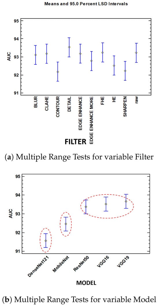
Figure 3.
Comparison of AUC under mean and 95.0 percent LSD intervals: (a) multiple range tests for variable filter, (b) multiple range tests for variable model [10].
Beeravolu et al. [11] developed advanced pre-processing techniques to enhance deep convolutional neural networks (D-CNNs) for mammographic image analysis, addressing the limitations of traditional machine learning methods that often yield false positives and negatives. The study proposes background and pectoral muscle removal methods, noise addition, and image enhancements. Specifically, the “Rolling Ball Algorithm” and “Huang’s Fuzzy Thresholding” achieve 100% background removal. Figure 4 shows the background removal treatment before and after comparison. Meanwhile, “Canny Edge Detection” and “Hough Line Transform” remove pectoral muscles in 99.06% of images.

Figure 4.
Final images after background removal process [11].
Additionally, image enhancements using “Invert”, “CTI_RAS”, and “ISOCONTOUR” lookup tables (LUTs) effectively delineate Regions of Interest (ROIs), and the enhancement effect is shown in Figure 5. These pre-processing techniques create high-quality, representative training data, improving the efficiency and accuracy of D-CNNs in real-world applications.
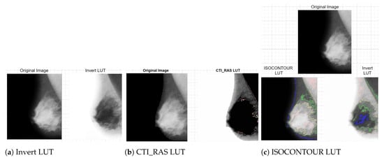
Figure 5.
Image enhancement technology applications [11].
2.2. Breast Cancer Detection
The early detection and precise diagnosis of breast cancer are paramount for effective treatment. Various breast screening methods have been developed to enhance detection, including mammography, breast ultrasound (BU), magnetic resonance imaging (MRI), computed tomography (CT), thermography, and biopsy. Mammography, the gold standard for early detection, utilizes X-ray images to identify abnormalities in the breast. Ultrasound, while non-invasive and suitable for patients with dense breast tissue, suffers from poor resolution and limited coverage. MRI offers high sensitivity in detection but is costly and less specific. Histopathology, although definite, requires large image sizes. Each modality’s distinct advantages and limitations underscore the critical importance of a multifaceted approach to the early detection of breast cancer [12].
Kandlikar and Satish G et al. in [13] indicate that microcalcifications (MCs) are essential indicators for detecting breast cancer in mammograms. Clustered MCs characterize malignant breast cancer with a linear branching pattern involving more than three MCs, each less than 0.5 mm in diameter. In contrast, benign conditions typically present as individual MCs. Figure 6 illustrates various common microcalcifications (MCs) identified in mammographic images, highlighting their diverse morphological characteristics.
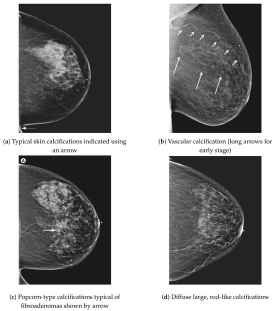
Figure 6.
Several common types of MCs observed in mammograms [14].
Breast lumps or masses are often indicative of breast cancer. Compared to normal or benign tissue, cancerous breast tissue is generally firmer. These lumps can be mobile but are usually fixed, meaning they feel attached to the skin or nearby tissue and cannot be moved by pressing them. They are typically painless, although pain may be present in some cases [15].
Zhang, Ya-nan and Xia, Ke-Rui et al. in [1] emphasize that early breast cancer detection can be enhanced by identifying tumor markers, which are substances released from tumor cells during their growth. Once these markers reach a detectable level, they can be extracted from breast images. Techniques such as the scale-invariant feature transform (SIFT) or the histogram of oriented gradients (HOG) can extract and analyze these early feature values, thereby supporting early diagnosis and potentially improving patient outcomes.
2.3. Image Segmentation
Segmentation is performed after classification to improve the interpretability and localization of anomalies detected within breast images, serving as a crucial step for the precise boundary delineation of lesions. While classification identifies the presence of abnormalities, segmentation delineates the exact contours of these lesions, thereby enhancing the granularity and specificity of the analysis. This process enables a more targeted approach to diagnostic decision-making by ensuring that the detected regions align accurately with the actual areas of clinical concern. The precision offered via segmentation is essential not only for subsequent clinical evaluations but also for treatment planning, in which accurately localized information can directly impact therapeutic outcomes.
Michael E et al., in [16], divide classical segmentation theory into three primary categories: region methods (RMs), threshold methods (TMs), and edge methods (EMs), as shown in Table 1. Region methods offer robust segmentation in structured images but are less effective with noise. Threshold methods are computationally efficient but struggle with varying image conditions. Edge methods excel at boundary detection but may fail with weak or irregular edges. Overall, selecting a segmentation method depends on the specific characteristics and requirements of the mammogram images being analyzed.

Table 1.
Summary of merits and demerits of mammograms’ classical segmentation methods [16].
Gu P et al., in [17], address the challenge of accurately segmenting three-dimensional (3D) ultrasound images for breast cancer diagnosis, emphasizing the need for automated methods due to the impracticality and inconsistency of manual segmentation. The proposed solution involves a three-stage process: morphological reconstruction to reduce speckle noise and enhance image features, Sobel operator-based image segmentation to delineate tissue boundaries, and region classification based on size and mean intensity to categorize tissues into fat, fibroglandular, and cyst/mass types.
The main processing steps are shown in Figure 7. Figure 7a: A grayscale image slice. The top yellow arrow shows the position of a cyst. The bottom yellow arrow indicates a shadow artifact. The following operations are performed in 3D; these images are only one slice of the whole image stack. Figure 7b: Morphological reconstruction in 3D space. Figure 7c: Application of a 3D Sobel operator on the images. Figure 7d: Watershed segmentation in 2D image space. The two arrows are in the same positions as in Figure 7a, showing that the artifact is distinguished from the cyst during pre-processing. Figure 7e: Magnified view of watershed boundaries. White pixels are the boundaries of individual watershed regions. Figure 7f: Tissue-specific region classification result.

Figure 7.
Main stages of the proposed method [17].
Automated segmentation shows good congruence with manual segmentation while conserving detailed structures; a sample comparison diagram is shown in Figure 8. The red contours are from manual segmentation, and the blue contours are from automated segmentation.

Figure 8.
Comparison of manual and automated segmentation of fibroglandular tissues [17].
Experimental results using 21 breast ultrasound cases demonstrated an accuracy of 85.7% and an overlap ratio of 74.54% with manual segmentation. Despite its effectiveness, limitations include challenges with shadow artifact handling, the occasional need for manual correction, and validation on a small dataset. Overall, the automated method shows promise for improving consistency and accuracy in breast cancer diagnosis, but it requires further research to enhance its robustness and applicability.
Xu Y et al., in [18], again address the challenge of segmenting three-dimensional (3D) breast ultrasound images for breast cancer diagnosis using machine learning, highlighting the limitations of manual segmentation due to its subjectivity and time consumption. The proposed method employs convolutional neural networks (CNNs) for automatic segmentation into four major tissue types: skin, fibroglandular tissue, mass, and fatty tissue. The methodology involves training CNNs on manually annotated data to classify tissue types based on pixel-centric patches from orthogonal image planes.
The segmentation process is shown in Figure 9, where an eight-layer CNN (CNN-I) was designed for pixel-level patch classification with 128 × 128 image patches as input. The network processes the input through three convolutional layers, three pooling layers, one fully connected layer, and one softmax layer, and it uses the ReLU activation function after each convolutional and each fully connected layer. For a comprehensive evaluation of target pixel classification, a smaller CNN (CNN-II) was developed. CNN-II takes the output of CNN-I as input and processes it through one convolutional layer, one fully connected layer, and one soft-maximum layer to arrive at the final classification result of the target pixel. Evaluation metrics, including accuracy, precision, recall, and F1-measure, all exceeded 80%, with the Jaccard similarity index (JSI) reaching 85.1%, outperforming the previous watershed algorithm study, which achieved 74.54%. Despite its effectiveness, challenges remain, such as handling ultrasound artifacts and improving computational efficiency.
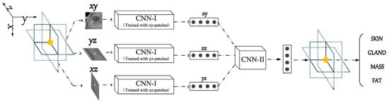
Figure 9.
The segmentation process in convolutional neural networks [18].
2.4. Machine Learning
Sadoughi F et al. [19] provide a comprehensive review of AI methods applied to breast cancer diagnosis, focusing on the high accuracy achieved using support vector machines (SVMs) across various imaging techniques, including ultrasound, mammography, and thermography. They underscore the role of AI in reducing false positives and enhancing radiologists’ efficiency in detecting breast abnormalities.
Mehdy M et al. [20] highlight the role of artificial neural networks (ANNs) in automating the classification of breast cancer images, which significantly reduces the time required for manual diagnosis and improves specificity and sensitivity. Their review of recent literature demonstrates the versatility of ANNs in various medical imaging applications, particularly in distinguishing between benign and malignant patterns.
Sahni and Mital [21] explored image processing techniques such as edge detection and thresholding in mammograms and MRI to improve tumor detection accuracy. They emphasize the critical role of early detection in improving treatment outcomes and reducing the complexity of medical interventions. Sadhukhan S et al. [22] propose a texture segmentation-based approach to analyzing digital mammograms, effectively distinguishing early-stage tumors using machine learning techniques and clustering algorithms. This method enhances the detection of masses and microcalcifications, which are crucial for early diagnosis.
Robertson S et al. [23] review the evolution of digital image analysis in breast pathology, particularly the transformative impact of AI and deep learning. They highlight how these technologies have improved diagnostic precision, facilitated personalized treatment, and addressed the increasing complexity of cancer pathology. The digitization of pathology data has enabled faster, more reproducible, and more accurate diagnoses, essential for guiding breast cancer treatment. It compares traditional medical image recognition and deep learning-based techniques, as shown in Figure 10.
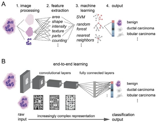
Figure 10.
Deep learning vs. traditional machine learning. (A) Traditional paradigm with several steps requiring expert human knowledge to recognize cancer in images. (B) Deep learning as an end-to-end approach from raw input image to classified image [23].
Atban F et al., in [24], address the problem of the accurate and early diagnosis of breast cancer through histopathological image classification, a critical challenge in the medical field due to the vast number of medical images and the complexity of manual classification. The study proposes a novel approach that combines transfer learning with meta-heuristic algorithms to optimize deep features for better representation and classification. The methodology involves using the ResNet18 architecture (Figure 11) for initial feature extraction, followed by the application of particle swarm optimization (PSO), atom search optimization (ASO), and equilibrium optimizer (EO) algorithms to select the most representative features. The optimized features are then classified using traditional machine learning algorithms like support vector machine (SVM), K-nearest neighbor (KNN), and decision trees (DTs). The approach is validated on the BreakHis dataset, achieving an F-score of 97.75% with ResNet18-EO and SVM and significantly improving classification performance.
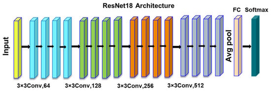
Figure 11.
ResNet18 architecture.
Chen H et al., in [25], establish predictive models based on algorithms like XGBoost, random forest, logistic regression, and K-nearest neighbor (KNN) to classify and predict breast cancer. The methodology involves data standardization to mitigate the impact of different data dimensions, feature selection using the Pearson correlation coefficient, and stratified sampling to handle the imbalance in positive and negative samples. The models are evaluated using metrics such as accuracy, precision, recall, and -score, with recall being the primary focus due to its significance in medical diagnostics. This paper compares the performance of each model when the dataset is split into training and testing sets with proportions of 8:2 (Table 2) and 7:2 (Table 3), respectively. The study finds that the XGBoost model, with an 8:2 training–test set division, performs the best, achieving a recall of 1.00 and an -score of 0.980.
Table 2.
The model effect of dividing the dataset by 8:2 [25].
Table 3.
The model effect of dividing the dataset by 7:3 [25].
2.5. Deep Learning
Researchers have recently integrated machine learning methods with feature selection techniques to evaluate their effectiveness in classification and segmentation tasks. For breast cancer detection and early diagnosis, Zheng et al. [26] propose a deep learning-assisted AdaBoost method. By using convolutional neural networks, the ensemble classifier significantly enhances system performance, showing potential for rapid adoption and improved predictive results. [27] presents a method for breast cancer classification and detection that integrates machine learning and image processing techniques. The method involves image preprocessing using a geometric mean filter, feature extraction with AlexNet, and feature selection with the relief algorithm. For classification and detection, the model employs various machine learning algorithms, including a least squares support vector machine (LSSVM), k-nearest neighbors (KNN), random forest (RF), and naive Bayes (NB). Experimental studies demonstrate that this method excels in accurately identifying breast cancer through image analysis.
Ho DJ et al., in [28], address the problem of accurate multi-class tissue segmentation in whole slide images (WSIs) of breast cancer, an essential step for effective diagnosis and treatment planning. The proposed solution is a deep multi-magnification network (DMMN) that integrates patches from multiple magnifications (20×, 10×, and 5×) to enhance segmentation accuracy by capturing both cellular details and architectural patterns, as shown in Figure 12. The methodology involves the partial annotation of WSIs to reduce labeling efforts, the extraction of multi-magnification patches, and class balancing using elastic deformation to ensure sufficient training data for rare classes. The DMMN architecture features multiple encoders and decoders with intermediate layer concatenations to fully utilize feature maps from different magnifications. This approach outperforms single magnification networks and other multi-magnification methods by achieving a higher mean intersection-over-union (mIOU), as well as higher recall and precision. However, the model’s performance is limited when segmenting well-differentiated carcinomas due to their absence from the training dataset, highlighting the need for more comprehensive training data to cover diverse cancer morphologies.

Figure 12.
Introduction of a deep single-magnification network (DSMN) and a deep multi-magnification network (DMMN) for the tissue segmentation of whole slide images [28].
Jiang J et al., in [29], address the challenge of accurate breast cancer detection and classification in mammograms, aiming to improve diagnostic efficiency and reduce false positives. Their paper introduces a three-stage deep learning framework utilizing a probabilistic anchor assignment (PAA) algorithm, as shown in Figure 13. The methodology involves a PAA-based detector to identify suspicious lesions, followed by a two-branch ROI detector to reduce false positives. Finally, classifiers are used to determine whether lesions and whole mammograms are benign or malignant. The framework combines local-ROI and global-image features to enhance accuracy. However, the model faces limitations in handling dense breast tissues, and it requires further optimization for post-processing algorithms. Additionally, multi-view inputs could potentially improve performance.
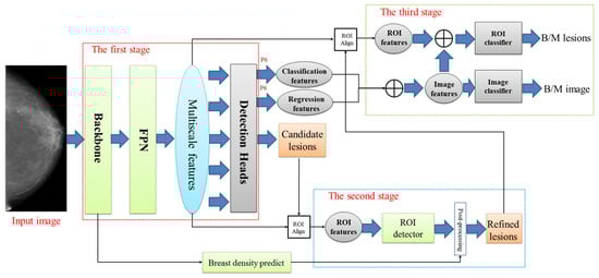
Figure 13.
The framework for our proposed three-stage deep learning model [29].
Yan et al., in [30], address the critical issue of accurately classifying breast cancer via deep learning techniques applied to breast ultrasound (BUS) images. The study proposes a sophisticated computer-aided diagnosis (CAD) framework named the Multistage Feature Distillation Network (MFD-Net). This framework leverages a convolutional neural network (CNN) to extract multilevel features from BUS images through depthwise separable convolution, enhancing fine-grained image feature distillation. The MFD-Net incorporates an innovative attention module with channel and spatial attention (Figure 14), improving classification accuracy by focusing on key image regions. The results showed that MFD-Net outperformed ten state-of-the-art models, achieving superior precision, recall, F1 scores, and accuracy. However, the reliance on a single dataset and potential variability in immunohistochemical results due to physician expertise are noted limitations.
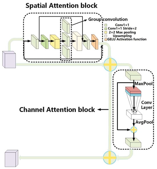
Figure 14.
Overall structure diagram of the ESCA attention mechanism [30].
3. Proposed Methods
In this section, we focus on the research techniques we chose, explaining each method from the perspectives of principles, the reasons for their selection, and their advantages, and we demonstrate how each method addresses the project’s concerns. Here, we list the datasets we plan to use, which include multiple types of imagery. We then introduce traditional image processing models, discussing image quality assessment methods, Wiener filtering, and total variation filtering. This lays the groundwork for a further exploration of how traditional processing can enhance the early diagnostic performance of artificial intelligence algorithms. Finally, we transition to artificial intelligence algorithms, introducing the latest Kolmogorov–Arnold network (KAN) architecture. We then discuss the challenges of early breast cancer diagnosis in terms of classification and image segmentation, introducing the Vit model and the Unet model and exploring the potential of combining the Unet model with the latest KANs framework to achieve superior performance. This combination is expected to yield improved results. For a detailed technical roadmap, refer to Figure 15.
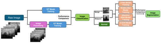
Figure 15.
Proposed methods’ workflow diagram.
3.1. Work Dataset Presentation
In this section, we detail the datasets utilized in our project aimed at AI-based early breast cancer detection and classification. The success of such a project heavily relies on the availability and diversity of relevant medical image datasets. Previous studies have highlighted a significant limitation in current AI-based early breast cancer diagnosis models, specifically their dependence on a single type of medical image, which leads to weak generalization across different datasets. To address this issue, we propose analyzing and training models using multiple datasets comprising multimodal medical images. The datasets employed in this research are shown in Table 4, including the Breast Ultrasound Images Dataset [31], MIAS Mammography [32], Mini-DDSM [33], BreakHis [34], and BreastDM [35]. These datasets encompass four mainstream medical image types: ultrasound, mammography, histopathological images, and DCE-MRI. By leveraging these diverse datasets, we aim to enhance the robustness and generalizability of AI models in early breast cancer detection and classification.
Table 4.
Selected dataset.
The selection of the five datasets—BreastDM, BUSI, MIAS, BreakHis, and DDSM—was implemented to comprehensively evaluate the proposed AI models across a wide range of imaging modalities and clinical scenarios in breast cancer detection. The BreastDM dataset, with 232 cases focused on the DCE-MRI domain, provides a robust foundation for both segmentation and classification tasks, offering a unique emphasis of MRI, which is critical for detecting tumors in dense breast tissue. The BUSI dataset introduces the challenges of ultrasound imaging, such as speckle noise and lower resolution, ensuring that the models are tested on imaging modalities where mammography might be less effective. The MIAS and DDSM datasets, both containing mammographic images with various abnormalities and tissue densities, are pivotal for assessing the models’ performance in one of the most widely used breast cancer screening methods. BreakHis, with its histopathological images, adds another layer of complexity by requiring the models to differentiate between benign and malignant tissues at the cellular level. By leveraging these datasets, the study not only covers a diverse spectrum of imaging types—each with its specific challenges—but also ensures that the models are robust, generalizable, and applicable across different clinical contexts, ultimately enhancing their potential utility in real-world breast cancer diagnostics.
3.2. Restoration Image Modeling
In medical imaging, the phenomenon of image degradation refers to the deterioration in the quality and clarity of images, which can adversely affect diagnostic accuracy. This degradation arises from various factors, including motion artifacts caused by patient movement, the technical limitations of imaging equipment, and noise from electronic interference or low signal strength. Additional factors include beam hardening in CT imaging, in which X-ray beams passing through denser tissues lead to artifacts and reduced contrast, and the partial volume effect, in which voxels containing multiple tissue types produce blurred images. The attenuation and scattering of signals in modalities such as ultrasound and MRI further contribute to degradation. The manifestations of these issues are evident in blurring, artifacts, noise, and contrast reduction, all of which impair the visibility and differentiation of anatomical structures. Understanding these causes and manifestations is essential for enhancing image acquisition techniques and developing methods to mitigate degradation, thereby improving the diagnostic utility of medical imaging.
To address the degradation caused by blurring, distortion, and noise in images, it is necessary to perform image restoration. Image restoration aims to recover the original appearance of a degraded image as closely as possible. This process involves reversing the degradation effects, which means that, if we know the specific processes that led to the degradation, we can restore the image by applying the inverse of these processes. The process of image degradation is shown on the left side of Figure 16.

Figure 16.
The general model for image restoration.
As illustrated in Figure 16, the image degradation model can be represented by Equation (1): The input image is convolved with the degradation function and subsequently linearly superimposed with noise to yield the degraded image. Through the application of a Fourier transform to this equation, the image degradation model can be expressed in the frequency domain as Equation (2).
where:
- is the input image.
- is the point spread function (PSF) that represents the blurring effects and other imperfections.
- is the noise added to the image.
- is the resulting degraded image.
- , , and are the Fourier transforms of , , and , respectively.
- is the Fourier transform of the degraded image .
In the initial analysis of the image recovery model, it becomes evident that different types of noise or blurring possess distinct functional expressions. Consequently, the effectiveness of various recovery filters varies, depending on the type of noise encountered. Understanding the characteristics of different types of noise is, therefore, crucial in selecting the appropriate image processing methods.
Article [36] provides a detailed explanation of the common types of noise found in medical imaging. Gaussian noise arises from atomic thermal vibrations and intermittent radiation from hot objects, as well as sensor noise due to temperature or brightness variations. Salt noise consists of randomly bright pixels (value 255), while pepper noise involves random dark pixels (value 0). Speckle noise, inherent in ultrasound images, is multiplicative and degrades diagnostic quality by reducing contrast and resolution. Poisson noise, resulting from the quantized nature of electromagnetic waves like gamma rays, X-rays, and visible light, introduces signal-dependent fluctuations as photons interact with the body. Thus, traditional additive noise removal techniques are ineffective for Poisson noise. The specific expressions are summarized in Table 5.
Table 5.
Common noise functions for medical imaging.
3.3. Image Quality Assessment
Image quality assessment (IQA) ensures that medical images meet the standards for accurate diagnosis and effective treatment, especially in early breast cancer detection. The three main types of IQA are Full-Reference (FR-IQA), Reduced-Reference (RR-IQA), and No-Reference (NR-IQA). Our research focuses on using appropriate IQA standards to evaluate the quality of our image processing results, aiming to obtain reliable, high-quality medical images for further analysis to improve the accuracy and sensitivity of early breast cancer diagnosis.
FR-IQA methods, such as the mean squared error (MSE), peak signal-to-noise ratio (PSNR), and structural similarity index (SSIM), require a pristine reference image for comparison. MSE measures the average squared differences between the original and distorted images, while PSNR provides a logarithmic scale of these differences. SSIM evaluates image quality based on structural information, luminance, and contrast, aligning closely with human visual perception. RR-IQA methods use partial information from the reference image to assess quality, balancing the need for reference data with evaluation accuracy. These techniques extract and compare specific features from both the reference and distorted images. NR-IQA, or blind IQA, is particularly valuable in medical imaging, for which reference images are often unavailable. The Blind/Referenceless Image Spatial Quality Evaluator (BRISQUE) is a prominent NR-IQA metric that assesses image quality based on natural scene statistics, operating in the spatial domain to quantify deviations from expected natural statistics.
Chow, Li Sze and Paramesran, Raveendran, in [37], mention that, in real-time medical imaging, there is no original or perfect reference image to evaluate. Therefore, NR-IQA becomes the most suitable method to evaluate medical images. Among NR-IQA methods, the BRISQUE method does not require the computation of specific distortion features; instead, it utilizes scene statistics of locally normalized luminance coefficients to quantify potential losses in the image’s ‘naturalness’. In terms of statistical performance, this method surpasses PSNR and SSIM, and it demonstrates high competitiveness and computational efficiency compared to other NR-IQA methods. Therefore, in this study, several evaluation criteria are employed: MSE, PSNR, SSIM, standard deviation (STD), and BRISQUE. MSE and PSNR provide foundational error measurements, while SSIM offers a perceptually aligned evaluation. STD captures image variability, and BRISQUE excels in scenarios lacking reference images. This comprehensive approach ensures rigorous and versatile IQA, providing reliable, high-quality medical images for further analysis to enhance the accuracy and sensitivity of early breast cancer diagnosis.
3.4. Wiener Image Filtering
The objective of image restoration is to estimate the original image from the observed degraded image and the degradation function , along with any available information about additive noise. The simplest approach to restoring an image could be implemented in the absence of noise, as follows:
This direct and simple method is known as inverse filtering, where is the Fourier transform of the estimated image. In practical scenarios, due to the presence of noise, directly applying this formula often results in the amplification of noise, leading to poor restoration. Therefore, according to Equation (2), Equation (3) can be modified under the condition of considering noise, giving the following:
When performing inverse filtering, if is very small or zero in certain areas while is not zero and relatively large, the second term in the equation can become significantly larger than the first term, leading to substantial errors. The Wiener filter is highly effective for this problem, as it is a form of linear minimum mean square error (LMMSE) estimation. Linear indicates that the estimation is linear in nature, while minimum variance refers to the optimization criterion used in constructing the filter. Specifically, it aims to minimize the variance of the error between the actual signal and the estimate (Equation (5)). The goal of the Wiener filter is to design a filter such that the output signal, obtained via filtering the observed signal, is the minimum mean square error estimate of the actual signal.
The Wiener filter, in its many variations, can be single-input–output or multiple-input–output, depending on the issue at hand with the image. However, the basic idea of Wiener filtering is still the same. A signal can be extracted from a mixture of signal and noise via filtering (in the form of a matrix or other model). So, the core of Wiener filtering is used to compute this filter (the parameters of the matrix r or model), thus solving the Wiener–Hopf equation. To facilitate the derivation of its principle, when assuming that the system is a single-input–output type and considering only finite-length filtering (i.e., considering that the signal at the current moment is only correlated with the signal at the previous finite number of time points), it can be seen from Figure 16 that, at this time, the output of the Wiener filter is as follows:
Following the derivation process detailed in Appendix A, we obtain the fundamental formula for the simplest single-input, single-output Wiener filter:
3.5. Total Variational Filtering
The previous subsection revealed that the Wiener filter is based on frequency-domain filtering, using the known noise and signal power spectrum. De-noising and de-blurring are achieved through inverse convolution, focusing on global noise suppression and blur correction, making it more suitable for dealing with linear and smooth noise. The total variation filter is based on the variational method. It focuses on retaining the edges by minimizing the total variation in the image in order to achieve denoising. Through the spatial domain of the iterative optimization of denoising and solving the nonlinear optimization problem, the noise can effectively be removed while retaining the edges.
Here is the simple derivation of the equation. The total variation filter constitutes an anisotropic model leveraging gradient descent to achieve image smoothing, with a primary objective of maximizing smoothness across the image domain by minimizing discrepancies between adjacent pixels while concurrently preserving edges to the utmost extent feasible. The term “variation” refers to , where approaches 0 for continuous functions. Total variation pertains to intervals defined for functions, where variations accumulate over the interval. Thus, by observing the definitions of the variation and the total variation of continuous real functions, we can derive equations for their discrete forms, specifically the total variation equation of one-dimensional discrete signals. For a discrete signal sequence , the total variational form of the one-dimensional discrete signal is given by Equation (8).
Upon obtaining the observed signal x, the objective is to smooth x, effectively denoising it. An intuitive approach is to minimize the total variation of the signal, which corresponds to the physical meaning of the input signal’s smoothness. Let the recovered signal be y, which should satisfy two conditions: y should not deviate significantly from the observed signal x (expressed as Equation (9)), and the total variation of y should be small. Under these constraints, y can be represented as in Equation (10), where the parameter is a positive constant used to balance the influence of the two constraints.
As early as 1992, Rudin et al. proposed the total variation equation for two-dimensional discrete signals (images) in Article [38], as shown in Equation (11). Solving this equation of total variation is relatively difficult; therefore, there is another commonly used definition for two-dimensional total variation (Equation (12)). The minimization problem of this equation is relatively simple to solve.
In this paper, we selected Wiener filtering and total variation (TV) filtering as our primary preprocessing techniques due to their complementary capabilities in addressing the dual challenges of noise reduction and edge preservation in breast cancer imaging. Wiener filtering was chosen for its effectiveness in mitigating Gaussian noise, which is a common issue across medical imaging modalities such as DCE-MRI and ultrasound. Its adaptive approach, based on the local mean and variance estimation, allows for significant noise reduction while preserving critical image details, making it particularly useful for enhancing the visibility of subtle tumor features.
To complement this, total variation filtering was employed in order to maintain the integrity of edge information, which is crucial for accurate tumor delineation in modalities like mammography and histopathology. TV filtering minimizes noise while preserving sharp transitions in an image, ensuring that essential structural details are retained.
Both filters were carefully optimized to align with the specific characteristics of each dataset. For Wiener filtering, the noise-to-signal ratio was fine-tuned to balance noise reduction with the preservation of tissue contrast, which is especially important in DCE-MRI and ultrasound. Similarly, the regularization parameter in TV filtering was adjusted to prioritize edge preservation while achieving effective noise suppression, particularly in datasets in which clear tumor boundaries are critical.
The strategic combination and optimization of these two filtering techniques enhance the overall image quality, providing the AI models with superior input data that supports improved performance and generalizability across diverse imaging modalities.
3.6. Kolmogorov–Arnold Networks
Traditional multilayer perceptrons (MLPs) have achieved significant success in machine learning but face challenges such as large parameter counts and limited interpretability. To address these issues, Liu and Wang et al., in the article [39], propose the Kolmogorov–Arnold network (KAN), a novel neural network architecture designed to enhance model flexibility and expressiveness while maintaining interpretability.
KAN’s design is inspired by the Kolmogorov–Arnold representation theorem, as shown in Equation (13), which posits that a multivariate, continuous function can be decomposed into a finite composite of univariate continuous functions and binary additive operations. Instead of using fixed activation functions at the nodes, KAN employs learnable activation functions at the network’s edges. This allows each weight parameter to be replaced with a univariate function, typically parameterized as a spline function. By applying learnable activation functions to the weights, KAN can more flexibly and accurately capture complex relationships in input data.
Figure 17 illustrates a structural comparison between multilayer perceptrons (MLPs) and Kolmogorov–Arnold networks (KANs). The primary distinction lies in the sequence of operations: MLP applies linear combinations followed by nonlinear activations, whereas KAN employs nonlinear activations for each input prior to the linear combinations. Crucially, KAN features parameterizable and learnable activation functions, unlike fixed functions like Sigmoid or ReLU in MLP. This adaptability enables KAN to represent complex curves with greater efficiency, thereby achieving higher accuracy with fewer parameters.
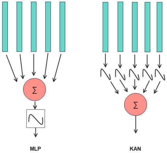
Figure 17.
Comparison of MLP and KAN structure.
Theoretically, two KAN layers (one representing the inner function and one learning the outer function) are sufficient to model various supervised learning tasks over the real number domain. This is analogous to the Kolmogorov–Arnold (KA) representation theorem. However, the activation functions in KANs can sometimes become very non-smooth, making it difficult to approximate any function using smooth splines in practice. Hence, the necessity for multi-layer KANs arises. Unlike the KA theorem, which restricts each input to produce nonlinear activations, as indicated in Equation (13), KANs can be more flexible and stacked to form deeper networks, resulting in more practical activation functions. The essence of deep learning is representation learning, which involves composing simple modules to learn complex functions. Therefore, extending KANs to multiple layers aligns with this principle. In article [39], a KAN layer with -dimensional inputs and -dimensional outputs is defined as a matrix of one-dimensional functions using the following equation:
To further compute , we can use the Equation (15); each value from the l-th layer corresponds to an activation function for . After processing each value through the corresponding activation function, we simply sum them up to get .
As shown in Figure 18, the two-layer KANs in the article [39] have the 0-th layer (bottom) representing the inner function, changing the variable dimensionality from n to . The first layer represents the outer function, changing the dimensionality from to 1 and resulting in a real number. Extending the basic two-layer KANs to a general form,
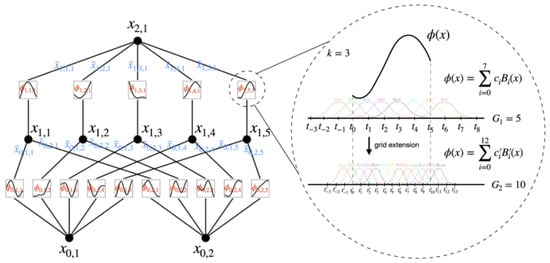
Figure 18.
Two-layer KANs [39].
3.7. U-Net
The UNet algorithm is a convolutional neural network (CNN) architecture for image segmentation. It was proposed by Olaf Ronneberger et al. in [40], and it is mainly used to solve the problem of medical image segmentation. The key innovation of UNet is its U-shaped architecture, which allows for high segmentation accuracy even with a limited number of training images.
UNet is a fully convolutional neural network for image segmentation, comprising an encoder and a decoder. The encoder extracts features using convolutional layers and pooling operations, reducing spatial resolution while capturing crucial details. The decoder then upsamples these low-resolution, high-level feature maps, combining them with corresponding encoder feature maps via skip connections. This technique enhances segmentation accuracy and detail preservation by utilizing both high-level abstract and low-level detailed features.
In the final stage, two convolutional layers generate feature maps, followed by 1 × 1 convolutions to produce class-specific heatmaps. The softmax function processes these heatmaps to compute probabilities, which are then used for loss calculation and backpropagation.
The UNet algorithm excels in segmentation and is well suited to small-sample learning, but it demands high computational resources and faces challenges with data imbalance and large image processing. The article [41] notes that, despite various innovative enhancements incorporating transformers or MLPs, these networks remain constrained due to linear modeling paradigms, and they lack sufficient interpretability. To address these problems, Li, Chenxin, Liu, Xinyu, et al. proposed the U-KAN architecture, as illustrated in Figure 19. This design incorporates elements from KANs, which are renowned for its high accuracy and interpretability. KANs transform neural network learning by incorporating nonlinearly learnable activation functions derived from the Kolmogorov–Arnold representation theorem.
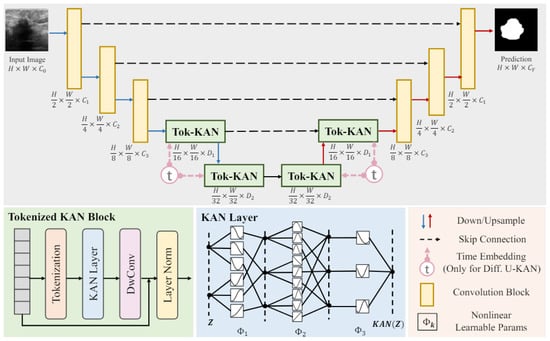
Figure 19.
U-KAN architecture [41].
The U-KAN architecture consists of a two-phase encoder–decoder structure. The encoder phase starts with three convolutional blocks that progressively reduce the feature map resolution, followed by two tokenized Kolmogorov–Arnold network (Tok-KAN) blocks. Conversely, the decoder phase includes two Tok-KAN blocks and three convolutional blocks that restore the feature map resolution. Skip connections link corresponding blocks in the encoder and decoder to facilitate feature reuse. Channel counts for the convolution and Tok-KAN phases are defined by hyperparameters C1 to C3 and D1 to D2, respectively. This architecture effectively integrates convolutional and tokenized KAN blocks, enhancing segmentation accuracy and interpretability and setting it apart from conventional UNet designs.
3.8. Vision Transformer
The vision transformer (ViT), developed by Google, repurposes the transformer architecture for computer vision tasks using an attention mechanism. While CNNs have traditionally been the cornerstone for computer vision, transformers are primarily used in NLP for tasks such as translation and text generation. Researchers have adapted the transformer’s multi-head self-attention to vision tasks in order to address the limitations of CNNs in capturing long-range dependencies. ViT has proven effective in image classification, object detection, and segmentation by leveraging its capability to process images of varying scales and resolutions and capture global contextual information.
The vision transformer (ViT) architecture (Figure 20), designed for computer vision tasks, consists of three main modules. The Linear Projection of Flattened Patches module converts input images into a serialized format suitable for the transformer encoder using the incorporating patch, position, and learnable embeddings. The transformer encoder, the core component, utilizes multi-head self-attention and feed-forward neural networks to capture global information and learn feature representations. Finally, the MLP head processes the output from the transformer encoders using a multi-layer perceptron for classification or other vision tasks.
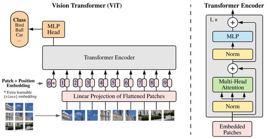
Figure 20.
Vision transformer architecture. In order to perform classification, the standard approach of adding an extra learnable “classification token” to the sequence is used (shown by ∗) [42].
The ViT model starts by segmenting an input image into fixed-size patches, which are then linearly transformed into lower-dimensional patch embeddings. Positional and learnable embeddings are added to retain spatial and global information. These embeddings are input to multiple layers of transformer encoders, which apply self-attention to extract features. The final output vectors are processed through a fully connected layer for classification. By converting image data into a sequence format, ViT effectively leverages the transformer’s attention mechanisms for efficient image analysis and classification.
3.9. Comparative Analysis with Previous Works
The application of machine learning and deep learning techniques to breast cancer detection has been extensively explored, yet challenges related to generalizability across different imaging modalities remain significant. Previous methods, such as those proposed in [21], focused on specific imaging modalities like mammography and MRI and on employing traditional image processing techniques such as edge detection and thresholding. These methods have shown efficacy within their targeted applications; however, their adaptability to other imaging modalities is limited. For instance, while edge detection may work effectively in mammography by highlighting distinct boundaries, it often fails to capture the more nuanced variations present in ultrasound images, where tissue interfaces are less clear. Similarly, thresholding techniques that perform well in MRI may not adequately handle the complex textures seen in histopathological images, where contrasts between different tissue types can be subtle and varied.
In contrast, studies like [10] examined a broad range of deep learning architectures combined with various preprocessing techniques, placing significant emphasis on the architecture’s influence on model accuracy. However, these studies did not sufficiently explore how different preprocessing techniques affect performance across various imaging modalities, leading to limited generalizability. Our approach differs by systematically applying preprocessing techniques, specifically Wiener filtering and total variation filtering, across multiple modalities, including DCE-MRI, ultrasound, mammography, and histopathology. This strategic use of preprocessing enhances image quality uniformly across different datasets, thereby improving the overall performance and generalizability of AI models, which is an area where previous studies have often fallen short.
Moreover, by systematically applying image processing techniques, we are able to enhance the generalizability of AI models. Traditional approaches often rely on a one-size-fits-all strategy for preprocessing, which may not account for the nuanced differences between imaging modalities. Our method diverges from this by optimizing the filtering parameters for each dataset, ensuring that the preprocessing is tailored to the specific characteristics of the imaging data. This tailored approach not only improves the diagnostic accuracy within each modality but also enhances the robustness of the models when applied to diverse datasets.
Overall, the proposed method addresses the ongoing challenge of developing generalizable and robust diagnostic models applicable across multiple imaging modalities. By strategically applying advanced preprocessing techniques and integrating state-of-the-art AI models, this study seeks to offer an approach that navigates some of the limitations observed in previous methodologies. While further validation and exploration are needed, the findings presented here contribute to the ongoing dialog in the field, with the potential to inform future developments in breast cancer diagnostics.
3.10. Highlight of the Proposed Methods
The proposed method distinguishes itself through a comprehensive approach that integrates advanced preprocessing techniques with cutting-edge AI models. Key aspects include the following:
- 1.
- Multimodal dataset utilization: Unlike previous approaches that primarily focus on single-modality datasets, our method leverages a diverse range of medical imaging datasets. This strategy ensures that the AI models developed are robust and generalizable across various imaging conditions, enhancing their applicability in different clinical scenarios.
- 2.
- Advanced image processing techniques: By systematically comparing and integrating Wiener filtering with total variation filtering, our approach is designed to tackle specific challenges inherent to medical imaging, such as noise reduction and edge preservation. These challenges are crucial for improving image quality before applying AI models. Additionally, we tailor filtering parameters to the characteristics of each specific dataset, thereby enhancing the adaptability and performance of the models across different imaging modalities.
- 3.
- Integration of ViT and U-KAN models: The incorporation of vision transformer (ViT) and U-KAN models represents an innovative application in the context of breast cancer detection. These models have demonstrated superior performance in both classification and segmentation tasks when compared to traditional CNN-based models. Their integration provides a more robust and interpretable framework capable of being effectively applied across a variety of imaging modalities.
4. Experimental Results and Discussion
4.1. Results of Image Filtering
Assuming that the degraded features in the mammographic images of the dataset are due to Gaussian blur, this study utilized specific Python modules to estimate the Gaussian blur kernel and employ a Wiener filter to deblur the images. The implementation of this functionality requires a manual estimation of the Gaussian kernel. The Gaussian blur kernel function in image processing is defined by two primary variables: kernel size and standard deviation. The kernel size, represented as a pair of integers (k_width, k_height) or a single integer for square kernels, specifies the dimensions of the Gaussian kernel and determines the number of pixels considered around each target pixel when applying the blur. A larger kernel size results in a more extensive blur by averaging values over a wider area. The standard deviation sigma controls the spread or width of the Gaussian function, influencing the degree of blur. It dictates how much neighboring pixels affect the center pixel, with a larger sigma producing a broader, smoother blur and a smaller sigma resulting in a sharper, more localized blur. Often, a single standard deviation value is used for both the x and y directions to maintain a uniform blur effect. The setting of the Gaussian kernel is closely related to the final deblur effect.
In order to realize the subsequent early classification and diagnosis research, we set the parameters to an interval range, taking the Gaussian kernel size to be 3–9 with a step size of 2 and sigma to be 0.5–3.0 with a step size of 0.25. We calculated the optimal parameter selection under the current image database through image quality assessment (IQA) for subsequent research. This section demonstrates the processed images, all based on the MIAS database (https://www.mammoimage.org/databases/ (accessed on 20 July 2024)).
The processing effect of the Wiener filter under different variables is shown in Figure 21. We calculated the image quality evaluation metrics PSNR, SSIM, MSE, and BRISQUE to find the better variable settings under this dataset.
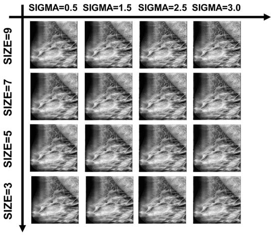
Figure 21.
Examples of Wiener filtering effects with partial variable combinations.
In Figure 22, Figure 23, Figure 24, Figure 25 and Figure 26, the Wiener filter’s performance across various image quality metrics—PSNR, SSIM, MSE, STD, and BRISQUE—reveals that the choice of kernel size and sigma significantly influences the quality of the denoised images. Optimal image quality, indicated by higher PSNR and SSIM values and lower MSE and BRISQUE scores, is generally achieved with smaller kernel sizes (3 to 4) and lower sigma values (0.5 to 1.0). Under these conditions, the filter effectively reduces noise while preserving structural details and minimizing deviations from the original image. As the kernel size and sigma increase, there is a noticeable decline in PSNR (from around 23 dB to 15 dB) and SSIM (from approximately 0.55 to 0.2), reflecting a loss of detail and structural fidelity. Concurrently, MSE values escalate (from around 250 to over 2250), highlighting increased error due to excessive smoothing.

Figure 22.
PSNR assessment of Wiener-filtered images.
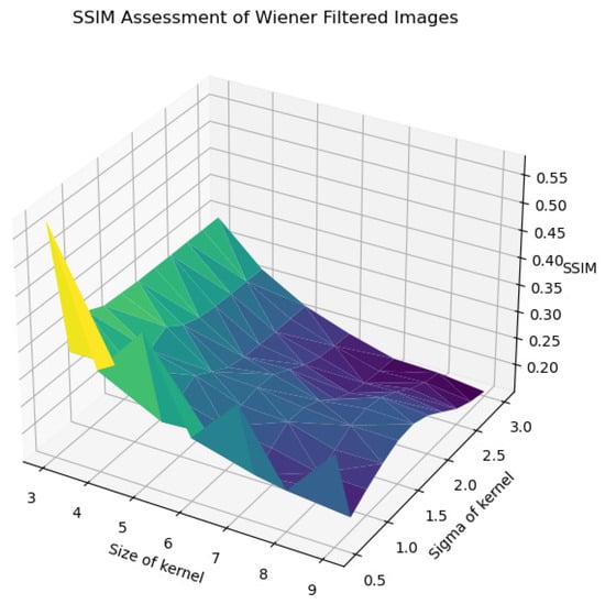
Figure 23.
SSIM assessment of Wiener-filtered images.

Figure 24.
MSE assessment of Wiener-filtered images.
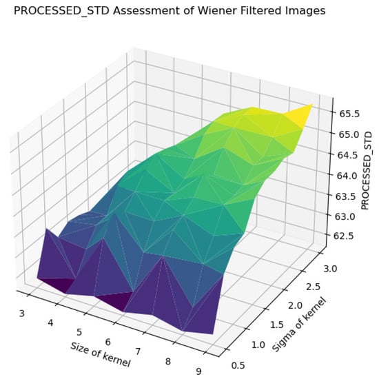
Figure 25.
STD assessment of Wiener-filtered images.
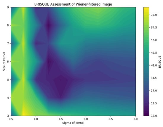
Figure 26.
BRISQUE assessment of Wiener-filtered images.
Furthermore, the standard deviation (STD) and BRISQUE metrics show a similar trend, where larger kernels and higher sigma values lead to increased uniformity and perceived quality degradation. The STD values rise from 62.5 to 65.5, indicating a reduction in texture variability, while BRISQUE scores increase from 12 to 72, suggesting diminished visual quality. These findings suggest that, while larger kernels and higher sigma values may be effective for noise reduction, they also introduce substantial over-smoothing, resulting in a loss of crucial image details and texture. Therefore, the careful selection of kernel size and sigma is essential for optimizing image quality, particularly in applications requiring a balance between noise suppression and the preservation of fine details for accurate early classification and diagnosis.
The analysis of the contour map of BRISQUE values in relation to kernel size and sigma parameters for Wiener-filtered images reveals distinct patterns. Smaller kernel sizes (3–5) are highly sensitive to variations in the sigma parameter, whereas larger kernel sizes (7–9) exhibit greater stability. Within the tested parameter range, a kernel size of 8 and a sigma value of 1.25 yield the best image quality, indicated by lower BRISQUE scores of 13.47. This combination effectively balances noise reduction and detail preservation. As shown in Figure 26, this specific combination results in the lowest BRISQUE score. Therefore, within the established range, these parameters are optimal for processing images in the current dataset. Through this method, we can determine the relatively optimal points within the assumed range of the dataset. The average evaluation metrics for the relatively optimal points within the parameter ranges of all used datasets are shown in Table 6. The optimal parameter sets for each dataset are as follows: for BreastDM, the optimal parameters (Size, Sigma) are (4, 3); for BreakHis, they are (5, 2.5); for DDSM, they are (5, 1.5); and for BUSI, they are (7, 1).
Table 6.
Assessment of Wiener filtering by IQA.
In addition, total variation filtering was applied to five datasets, with specific IQA parameters detailed in Table 7. It can be observed that, compared to Wiener filtering, the performance of total variation filtering is inferior. This is particularly evident in the BRISQUE parameter, which will likely significantly impact deep learning models. The substantial increase in BRISQUE values indicates a notable decline in image quality.
Table 7.
Assessment of total variation filtering by IQA.
Wiener filtering and total variation filtering are complementary in dealing with noise and preserving details. Wiener filtering is very effective in reducing Gaussian noise, while total variation filtering excels in preserving edges and details. Therefore, we processed images by applying total variation filtering to both the original dataset and the Wiener-filtered dataset and then evaluated the quality of the images, expecting that the processed images would lead to superior performance in early diagnosis for AI.
Table 8 shows the sample filtering effects for each dataset (the experimental settings are the same as the MIAS dataset, both assuming that the images are Gaussian blurred). Similar to the Wiener filter, the total variation filter has a different setup with the variable regularization parameter (), which controls the strength of the filtering and determines the balance between noise reduction and detail retention. Following the Wiener filter treatment, we explored the relatively optimal combination of parameters. Table 9 shows the evaluation metrics for each dataset under the relatively optimal parameters of the combined filters.
Table 8.
Comparison of filter processing effects in different datasets.
Table 9.
Assessment of combined filtering by IQA.
Figure 27, Figure 28 and Figure 29 use image quality assessment (IQA) metrics to compare the effects of different filtering techniques on various datasets. These datasets include MIAS (benign: 64 images; malignant: 51 images; normal: 207 images), BreakHis (benign: 2480 images; malignant: 5429 images), BUSI (benign: 437 images; malignant: 210 images; normal: 133 images), BreastDM (benign: 88 images; malignant: 147 images), and Mini-DDSM (benign: 671 images; malignant: 679 images, normal: 602 images). The metrics used are PSNR, SSIM (scaled by ), MSE (scaled by 10), and BRISQUE. These figures clearly illustrate the differences in image quality across different filtering methods, with particular emphasis on the BRISQUE metric, which indicates significant variations in image quality.
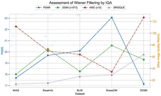
Figure 27.
Assessment of Wiener filtering by IQA.
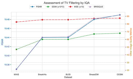
Figure 28.
Assessment of total variation filtering by IQA.
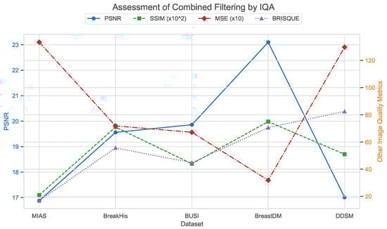
Figure 29.
Assessment of combined filtering by IQA.
4.2. AI Diagnostic Results
Evaluated using IQA metrics alone, Table 9 shows that the combined filter-treated images are degraded in all parameters. However, to draw accurate conclusions and validate whether Wiener filtering improves AI early diagnostic performance, we used five datasets, each subjected to three different treatments (including the original images), resulting in 15 different combinations for deep learning training. The primary task in the early diagnosis of breast cancer is to classify medical images to determine whether the condition is benign or malignant for targeted treatment. For the classification task, training was conducted using the VisionTransformer framework with a fixed 15 epochs for all datasets, a learning rate of 0.001, and a learning rate factor of 0.01. The performance of the same dataset under different treatments was compared and analyzed. Figure 30 illustrates the model training process data for the BUSI dataset.

Figure 30.
Comparison of the training process of the BUSI dataset with different treatments.
In Table 10, we analyzed the performance results of five different datasets after applying Wiener filtering and total variation filtering. It is evident that the performance varies significantly across different datasets, depending on the filtering technique used. For instance, in the Mini-DDSM dataset, although the performance of Wiener filtering and total variation filtering are relatively similar, the raw images perform the worst. However, the Breakhis dataset shows a significant performance improvement after applying Wiener filtering, particularly in accuracy, recall, and AUC.
Table 10.
Performance of five datasets with different treatments in the vision-transformer framework.
Further analysis reveals that the BreastDM dataset achieves the best results after applying Wiener filtering, with all performance metrics reaching their highest values. This indicates that our chosen range of parameters and parameter combinations are well suited to this dataset. The BUSI dataset exhibits excellent performance with both Wiener and total variation filtering, although Wiener filtering performs slightly better, suggesting that the effectiveness of different filtering methods varies across specific datasets.
Overall, these results indicate that filtering can significantly improve model performance in some cases but may have negative effects on certain datasets. Therefore, in practical applications, it is crucial to select the most appropriate image processing method based on the characteristics of the specific dataset to achieve optimal performance.
Further predictions using the trained model reveal more diverse performance outcomes. Figure 31 shows that, while the model can correctly classify images in the BreakHis dataset, there is a decrease in the likelihood of correctly classifying benign images post-processing, whereas the likelihood increases for malignant images. Figure 32 and Figure 33 demonstrate that filtered images significantly improve classification probabilities for the BreastDM and BUSI datasets. However, Figure 34 indicates that, despite improved accuracy and probability in processed images, the model misclassifies original DDSM images, which is critical in real diagnostics; specifically, a malignant image is diagnosed as benign with a probability of 0.504. Figure 35 illustrates a more severe issue in the MIAS dataset, where the model misclassifies benign images as normal with a probability of 0.421 (benign prob: 0.337; malignant prob: 0.242) and malignant images as normal with a probability of 0.526 (benign prob: 0.191; malignant prob: 0.283) after combined filtering. Image processing degraded the model’s classification performance with MIAS, and the original dataset’s classification probabilities were already low, indicating that the model is not well suited to the MIAS dataset.
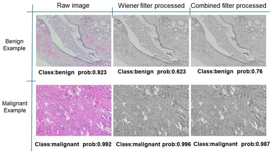
Figure 31.
Classification results in Breakhis.
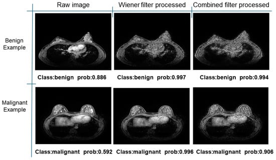
Figure 32.
Classification results in BreastDM.
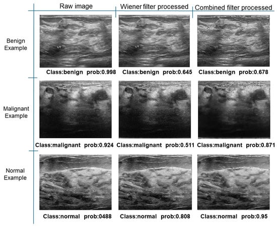
Figure 33.
Classification results in BUSI.
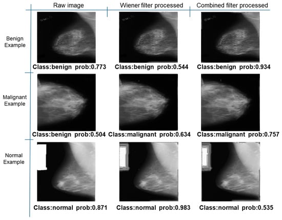
Figure 34.
Classification results in Mini-DDSM.
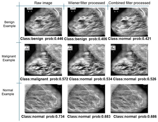
Figure 35.
Classification results in MIAS.
Table 11 presents a comparison between the mask images generated using three different frameworks and the ground truth masks for image segmentation. In Table 12, the performance comparison of various models on the BUSI and BreastDM datasets is presented, emphasizing their respective performance metrics. The methods for calculating performance metrics are detailed in Appendix A.
Table 11.
Comparison of different models using datasets.
Table 12.
Comparison of different models using datasets.
For the BUSI dataset, the U-KAN model demonstrates superior performance across most metrics relative to U-Net and U-Net++. Specifically, U-KAN achieves the highest accuracy (0.933), precision (0.754), and F1 score (0.747). Additionally, it records the highest specificity (0.963) and AUC (0.935), although its recall (0.740) is marginally lower than that of U-Net++ (0.749). These results indicate that U-KAN offers balanced and robust performance, excelling particularly in accuracy and specificity, which are critical for reliable image segmentation.
Regarding the BreastDM dataset, all three models exhibit high accuracy, yet U-KAN again shows the best overall performance. U-KAN achieves the highest accuracy (0.986), recall (0.870), F1 score (0.728), specificity (0.993), and AUC (0.838). In comparison, U-Net++ demonstrates slightly lower performance with an accuracy of 0.985 and an AUC of 0.822, while U-Net exhibits an accuracy of 0.983 and an AUC of 0.815.
These findings suggest that U-KAN is particularly effective for image segmentation tasks, especially in the context of early breast cancer diagnosis. It provides superior accuracy, specificity, and balanced performance across other metrics compared to U-Net and U-Net++, thus offering enhanced capabilities for detecting early-stage breast cancer lesions. Consequently, U-KAN’s advanced performance metrics underscore its potential as a reliable model for clinical applications in breast cancer detection.
5. Conclusions
This study systematically explored the effects of various image processing techniques and AI models on the performance of early breast cancer diagnostic systems. Experiments were conducted on multiple datasets, including BreastDM, BUSI, MIAS, BreakHis, and DDSM, ensuring a comprehensive evaluation across diverse medical image types. The results provided critical insights into the effectiveness of these techniques and models.
The application of Wiener filtering produced distinct image quality metrics across various datasets, as evidenced by measures such as the peak signal-to-noise ratio (PSNR), the structural similarity index measure (SSIM), the mean squared error (MSE), and the Blind/Referencel-ess Image Spatial Quality Evaluator (BRISQUE). With the BreastDM dataset, Wiener filtering achieved a PSNR of 23.06 dB, an SSIM of 0.79, and an MSE of 341.72, indicating effective noise suppression and good structural preservation, with a BRISQUE score of 28.88. For the BUSI dataset, Wiener filtering resulted in an SSIM of 0.35, a PSNR of 20.09 dB, and an MSE of 637.35, demonstrating moderate structural preservation and reasonable perceptual quality with a BRISQUE score of 26.23. In the MIAS dataset, Wiener filtering showed significant noise reduction with an MSE of 1114.22, a PSNR of 17.68 dB, and an SSIM of 0.30, maintaining perceptual quality with a BRISQUE score of 13.47. For the DDSM dataset, Wiener filtering achieved a PSNR of 17.14 dB, an SSIM of 0.55, and an MSE of 1267.13, reflecting moderate improvements and challenges in balancing noise reduction and perceptual quality with a BRISQUE score of 63.71. In the BreakHis dataset, Wiener filtering showed a PSNR of 19.69 dB, an SSIM of 0.73, and an MSE of 697.58, indicating good noise reduction and structural preservation, with a BRISQUE score of 15.12, suggesting good perceptual quality.
Combined filtering techniques produced mixed results that were highly dependent on the dataset. To evaluate their relative performance, these methods were compared against Wiener filtering. In the MIAS dataset, combined filtering decreased SSIM values from 0.30 (Wiener) to 0.21, reflecting potential over-enhancement issues. Additionally, MSE increased from 1114.22 (Wiener) to 1334.17 (combined), indicating slightly less effective noise reduction. The BRISQUE score increased from 13.47 (Wiener) to 16.87 (combined), suggesting a decrease in perceptual quality. Conversely, in the BUSI dataset, combined filtering significantly improved perceptual quality, as evidenced by a decrease in BRISQUE scores from 26.23 (Wiener) to 44.80 (combined). PSNR was slightly lower for combined filtering (19.86 dB) than Wiener filtering (20.09 dB) but still acceptable. SSIM improved from 0.35 (Wiener) to 0.44 (combined), indicating better structural preservation. This comparison indicates that, while Wiener filtering generally enhances image quality, combined filtering methods can offer additional benefits in specific contexts, especially for perceptual quality in datasets like BUSI.
The use of the vision transformer (ViT) framework provided a robust approach to evaluating the impact of different preprocessing techniques on AI diagnostic performance, particularly in the BreastDM and BUSI datasets. For the BreastDM dataset, the Wiener filter treatment achieved an accuracy of 96.9%, a precision of 97.2%, a recall of 96.7%, a specificity of 93.3%, and an AUC of 0.954. In comparison, the combined filter treatment yielded an accuracy of 99.3%, a precision of 99.6%, a recall of 98.3%, a specificity of 95.4%, and an AUC of 0.969, demonstrating superior performance. The raw image treatment showed lower metrics with an accuracy of 90.6%, a precision of 90.6%, a recall of 90.8%, a specificity of 93.3%, and an AUC of 0.937. For the BUSI dataset, the Wiener filter treatment resulted in an accuracy of 98.0%, a precision of 98.8%, a recall of 96.6%, a specificity of 98.5%, and an AUC of 0.998. The combined filter treatment had an accuracy of 83.2%, a precision of 81.1%, a recall of 79.2%, a specificity of 90.0%, and an AUC of 0.938, whereas the raw image treatment exhibited significantly lower performance with an accuracy of 71.6%, a precision of 74.8%, a recall of 61.6%, a specificity of 80.3%, and an AUC of 0.864. These results highlight the effectiveness of the ViT framework, particularly when combined with appropriate preprocessing techniques, in enhancing diagnostic accuracy and reliability.
The U-KAN model consistently outperformed the U-Net and U-Net++ models in breast cancer lesion segmentation across the datasets used. In the BUSI dataset, U-KAN achieved an accuracy of 93.3%, with a precision of 75.4%, a recall of 74.0%, an F1-score of 74.7%, a specificity of 96.3%, and an AUC of 0.935. These results indicate U-KAN’s robustness in accurately segmenting breast cancer lesions. Notably, with the BreastDM dataset, U-KAN maintained high segmentation accuracy with an accuracy of 98.6%, a precision of 62.6%, a recall of 87.0%, an F1-score of 72.8%, a specificity of 99.3%, and an AUC of 0.838 despite the presence of noise and variability in image quality. Furthermore, the U-KAN model’s ability to maintain high-performance metrics across these datasets underscores its adaptability and robustness.
In conclusion, this study underscores the importance of tailored preprocessing techniques for different datasets, given the variability in image quality and characteristics. Wiener filtering emerged as generally effective, particularly for datasets with significant noise, such as BreastDM. However, the choice of filtering techniques should be guided by the specific noise characteristics and diagnostic requirements of each dataset; for instance, combined filtering methods were more suitable in enhancing image clarity and feature preservation in the BUSI dataset. Integrating advanced AI models like ViT and U-KAN with optimal preprocessing techniques has proven to enhance diagnostic performance. The superior performance of the U-KAN model across various metrics suggests that combining innovative network architectures with tailored preprocessing can significantly improve early breast cancer detection. These findings highlight the need for further research to refine and validate these methods across larger and more diverse datasets.
Future work should address the challenge of selecting optimal parameters for different datasets, which remains difficult even when choosing a parameter range to find the best values. Integrating image processing with deep learning may offer a solution to this problem. By training models with various parameter combinations, it may be possible to achieve the adaptive selection of the optimal processing parameters. This approach could significantly enhance the performance of deep learning applications in early breast cancer detection, leading to more accurate and reliable diagnostic outcomes.
Author Contributions
Conceptualization, Z.Z. and B.H.S.A.; methodology, Z.Z. and B.H.S.A.; resources, B.H.S.A., Z.Z. and Y.S.; writing—original draft preparation, B.H.S.A., Z.Z. and Y.S.; writing—review and editing, B.H.S.A. and Z.Z.; supervision, B.H.S.A.; visualization, B.H.S.A. All authors have read and agreed to the published version of the manuscript.
Funding
This research received no external funding.
Data Availability Statement
Data are contained within the article.
Conflicts of Interest
The authors declare no conflicts of interest.
Appendix A. Some Theoretical Definitions
Appendix A.1. Wiener Filter
In order to ensure that the difference between the output, y, and the real signal, s, is minimized, and since y and s are temporal signals, it is important to ensure that the mean-square error is minimized for both of them, so the following is used:
To find the h that minimizes Equation (A1), taking the partial derivative of Equation (A1) with respect to h yields the following:
Setting the correlation coefficient between g and s is :
where denotes the correlation coefficient between and . Here, m is fixed, and j is varying, , denotes the correlation coefficient of , and . In the above equation, n denotes the time point in the sequence signal.
According to Equation (A4), the N-dimensional linear equation can be obtained:
Its matrix form is as follows:
From the previous model, it is known that the H matrix is the required filter parameter, which, in turn, leads to . At this time, the mean square error of the image is the smallest. According to Equations (A1) and (A4), we can obtain the following:
When signal s and noise n are independent of each other,
By substituting Equation (A7), we can obtain the basic formula of the simplest Wiener filter with a single input and output:
Appendix A.2. Image Quality and Classification Performance Metrics
- Peak signal-to-noise ratio (PSNR)where is the maximum possible pixel value of the image, and MSE is the mean squared error.
- Structural similarity index (SSIM)where and are the mean values of images x and y, , and are the variances, is the covariance, and and are constants for stabilization.
- Mean squared error (MSE)where I and K represent the pixel values of the original and compressed images, respectively, and m and n are the dimensions of the images.
- Blind/Referenceless Image Spatial Quality Evaluator (BRISQUE)where f is a function mapping Natural Scene Statistics (NSS) features to a quality score.
- Accuracywhere , , , and represent true positives, true negatives, false positives, and false negatives, respectively.
- Precision
- Recall
- Specificity
- Area under the curve (AUC)where is the true positive rate, and is the false positive rate.
References
- Zhang, Y.n.; Xia, K.R.; Li, C.Y.; Wei, B.L.; Zhang, B. Review of breast cancer pathologigcal image processing. BioMed Res. Int. 2021, 2021, 1994764. [Google Scholar] [CrossRef]
- Zerouaoui, H.; Idri, A. Reviewing machine learning and image processing based decision-making systems for breast cancer imaging. J. Med. Syst. 2021, 45, 8. [Google Scholar] [CrossRef] [PubMed]
- Khan, S.A.; Khan, M.A.; Song, O.Y.; Nazir, M. Medical imaging fusion techniques: A survey benchmark analysis, open challenges and recommendations. J. Med. Imaging Health Inform. 2020, 10, 2523–2531. [Google Scholar] [CrossRef]
- Khan, S.U.; Sharif, M.N.; Niass, M.I.; Afzal, M.; Shoaib, M. Comparison of multiple deep models on semantic segmentation for breast tumor detection. Found. Univ. J. Eng. Appl. Sci. 2021, 2, 12–23. [Google Scholar] [CrossRef]
- Honarvar Shakibaei Asli, B.; Zhao, Y.; Erkoyuncu, J.A. Motion blur invariant for estimating motion parameters of medical ultrasound images. Sci. Rep. 2021, 11, 14312. [Google Scholar] [CrossRef] [PubMed]
- Asli, B.H.S.; Flusser, J.; Zhao, Y.; Erkoyuncu, J.A.; Krishnan, K.B.; Farrokhi, Y.; Roy, R. Ultrasound image filtering and reconstruction using DCT/IDCT filter structure. IEEE Access 2020, 8, 141342–141357. [Google Scholar] [CrossRef]
- Kumar, N.; Nachamai, M. Noise removal and filtering techniques used in medical images. Orient. J. Comput. Sci. Technol. 2017, 10, 103–113. [Google Scholar] [CrossRef]
- Fan, L.; Zhang, F.; Fan, H.; Zhang, C. Brief review of image denoising techniques. Vis. Comput. Ind. Biomed. Art 2019, 2, 7. [Google Scholar] [CrossRef]
- Calvo, I.; Calderon, S.; Torrents-Barrena, J.; Muñoz, E.; Puig, D. Assessing the Impact of a Preprocessing Stage on Deep Learning Architectures for Breast Tumor Multi-Class Classification with Histopathological Images. In Proceedings of the High Performance Computing: 6th Latin American Conference, CARLA 2019, Turrialba, Costa Rica, 25–27 September 2019; pp. 262–275. [Google Scholar]
- Murcia-Gomez, D.; Rojas-Valenzuela, I.; Valenzuela, O. Impact of image preprocessing methods and deep learning models for classifying histopathological breast cancer images. Appl. Sci. 2022, 12, 11375. [Google Scholar] [CrossRef]
- Beeravolu, A.R.; Azam, S.; Jonkman, M.; Shanmugam, B.; Kannoorpatti, K.; Anwar, A. Preprocessing of breast cancer images to create datasets for deep-CNN. IEEE Access 2021, 9, 33438–33463. [Google Scholar] [CrossRef]
- Dar, R.A.; Rasool, M.; Assad, A. Breast cancer detection using deep learning: Datasets, methods, and challenges ahead. Comput. Biol. Med. 2022, 149, 106073. [Google Scholar]
- Kandlikar, S.G.; Perez-Raya, I.; Raghupathi, P.A.; Gonzalez-Hernandez, J.L.; Dabydeen, D.; Medeiros, L.; Phatak, P. Infrared imaging technology for breast cancer detection–Current status, protocols and new directions. Int. J. Heat Mass Transf. 2017, 108, 2303–2320. [Google Scholar] [CrossRef]
- Itani, M.; Griffin, A.T.; Whitman, G.J. Mammography of breast calcifications. Imaging Med. 2013, 5, 63. [Google Scholar] [CrossRef]
- American Cancer Society. Breast Cancer Signs and Symptoms. 2022. Available online: https://www.cancer.org/cancer/types/breast-cancer/screening-tests-and-early-detection/breast-cancer-signs-and-symptoms.html (accessed on 22 June 2024).
- Michael, E.; Ma, H.; Li, H.; Kulwa, F.; Li, J. Breast cancer segmentation methods: Current status and future potentials. BioMed Res. Int. 2021, 2021, 9962109. [Google Scholar] [CrossRef] [PubMed]
- Gu, P.; Lee, W.M.; Roubidoux, M.A.; Yuan, J.; Wang, X.; Carson, P.L. Automated 3D ultrasound image segmentation to aid breast cancer image interpretation. Ultrasonics 2016, 65, 51–58. [Google Scholar] [CrossRef] [PubMed]
- Xu, Y.; Wang, Y.; Yuan, J.; Cheng, Q.; Wang, X.; Carson, P.L. Medical breast ultrasound image segmentation by machine learning. Ultrasonics 2019, 91, 1–9. [Google Scholar] [CrossRef]
- Sadoughi, F.; Kazemy, Z.; Hamedan, F.; Owji, L.; Rahmanikatigari, M.; Azadboni, T.T. Artificial intelligence methods for the diagnosis of breast cancer by image processing: A review. Breast Cancer Targets Ther. 2018, 10, 219–230. [Google Scholar] [CrossRef] [PubMed]
- Mehdy, M.; Ng, P.; Shair, E.; Saleh, N.M.; Gomes, C. Artificial neural networks in image processing for early detection of breast cancer. Comput. Math. Methods Med. 2017, 2017, 2610628. [Google Scholar] [CrossRef]
- Sahni, P.; Mittal, N. Breast Cancer Detection Using Image Processing Techniques. In Proceedings of the Advances in Interdisciplinary Engineering: Select Proceedings of FLAME 2018; Springer: Berlin, Germany, 2019; pp. 813–823. [Google Scholar]
- Sadhukhan, S.; Upadhyay, N.; Chakraborty, P. Breast Cancer Diagnosis Using Image Processing and Machine Learning. In Proceedings of the Emerging Technology in Modelling and Graphics: Proceedings of IEM Graph 2018; Springer: Berlin, Germany, 2020; pp. 113–127. [Google Scholar]
- Robertson, S.; Azizpour, H.; Smith, K.; Hartman, J. Digital image analysis in breast pathology—From image processing techniques to artificial intelligence. Transl. Res. 2018, 194, 19–35. [Google Scholar] [CrossRef]
- Atban, F.; Ekinci, E.; Garip, Z. Traditional machine learning algorithms for breast cancer image classification with optimized deep features. Biomed. Signal Process. Control. 2023, 81, 104534. [Google Scholar] [CrossRef]
- Chen, H.; Wang, N.; Du, X.; Mei, K.; Zhou, Y.; Cai, G. Classification prediction of breast cancer based on machine learning. Comput. Intell. Neurosci. 2023, 2023, 6530719. [Google Scholar] [CrossRef]
- Zheng, J.; Lin, D.; Gao, Z.; Wang, S.; He, M.; Fan, J. Deep learning assisted efficient AdaBoost algorithm for breast cancer detection and early diagnosis. IEEE Access 2020, 8, 96946–96954. [Google Scholar] [CrossRef]
- Jasti, V.D.P.; Zamani, A.S.; Arumugam, K.; Naved, M.; Pallathadka, H.; Sammy, F.; Raghuvanshi, A.; Kaliyaperumal, K. Computational technique based on machine learning and image processing for medical image analysis of breast cancer diagnosis. Secur. Commun. Netw. 2022, 2022, 1918379. [Google Scholar] [CrossRef]
- Ho, D.J.; Yarlagadda, D.V.; D’Alfonso, T.M.; Hanna, M.G.; Grabenstetter, A.; Ntiamoah, P.; Brogi, E.; Tan, L.K.; Fuchs, T.J. Deep multi-magnification networks for multi-class breast cancer image segmentation. Comput. Med. Imaging Graph. 2021, 88, 101866. [Google Scholar] [CrossRef] [PubMed]
- Jiang, J.; Peng, J.; Hu, C.; Jian, W.; Wang, X.; Liu, W. Breast cancer detection and classification in mammogram using a three-stage deep learning framework based on PAA algorithm. Artif. Intell. Med. 2022, 134, 102419. [Google Scholar] [CrossRef] [PubMed]
- Yan, D.; Zhao, Z.; Duan, J.; Qu, J.; Shi, L.; Wang, Q.; Zhang, H. Deep learning-based immunohistochemical estimation of breast cancer via ultrasound image applications. Front. Oncol. 2024, 13, 1263685. [Google Scholar] [CrossRef]
- Al-Dhabyani, W.; Gomaa, M.; Khaled, H.; Fahmy, A. Dataset of breast ultrasound images. Data Brief 2020, 28, 104863. [Google Scholar] [CrossRef]
- Suckling, J. The Mammographic Images Analysis Society Digital Mammogram Database. Exerpta Medica 1994, 1069, 375–378. [Google Scholar]
- Lekamlage, C.D.; Afzal, F.; Westerberg, E.; Cheddad, A. Mini-DDSM: Mammography-Based Automatic Age Estimation. In Proceedings of the 2020 3rd International Conference on Digital Medicine and Image Processing, Kyoto, Japan, 6–9 November 2020; pp. 1–6. [Google Scholar]
- Spanhol, F.A.; Oliveira, L.S.; Petitjean, C.; Heutte, L. A dataset for breast cancer histopathological image classification. IEEE Trans. Biomed. Eng. 2015, 63, 1455–1462. [Google Scholar] [CrossRef]
- Zhao, X.; Liao, Y.; Xie, J.; He, X.; Zhang, S.; Wang, G.; Fang, J.; Lu, H.; Yu, J. BreastDM: A DCE-MRI dataset for breast tumor image segmentation and classification. Comput. Biol. Med. 2023, 164, 107255. [Google Scholar] [CrossRef]
- Kaur, A.; Dong, G. A complete review on image denoising techniques for medical images. Neural Process. Lett. 2023, 55, 7807–7850. [Google Scholar] [CrossRef]
- Chow, L.S.; Paramesran, R. Review of medical image quality assessment. Biomed. Signal Process. Control. 2016, 27, 145–154. [Google Scholar] [CrossRef]
- Rudin, L.I.; Osher, S.; Fatemi, E. Nonlinear total variation based noise removal algorithms. Phys. D Nonlinear Phenom. 1992, 60, 259–268. [Google Scholar] [CrossRef]
- Liu, Z.; Wang, Y.; Vaidya, S.; Ruehle, F.; Halverson, J.; Soljačić, M.; Hou, T.Y.; Tegmark, M. Kan: Kolmogorov-arnold networks. arXiv 2024, arXiv:2404.19756. [Google Scholar]
- Ronneberger, O.; Fischer, P.; Brox, T. U-net: Convolutional Networks for Biomedical Image Segmentation. In Proceedings of the Medical Image Computing and Computer-Assisted Intervention—MICCAI 2015: 18th International Conference, Munich, Germany, 5–9 October 2015; pp. 234–241. [Google Scholar]
- Li, C.; Liu, X.; Li, W.; Wang, C.; Liu, H.; Yuan, Y. U-KAN Makes Strong Backbone for Medical Image Segmentation and Generation. arXiv 2024, arXiv:2406.02918. [Google Scholar]
- Dosovitskiy, A.; Beyer, L.; Kolesnikov, A.; Weissenborn, D.; Zhai, X.; Unterthiner, T.; Dehghani, M.; Minderer, M.; Heigold, G.; Gelly, S.; et al. An image is worth 16 × 16 words: Transformers for image recognition at scale. arXiv 2020, arXiv:2010.11929. [Google Scholar]
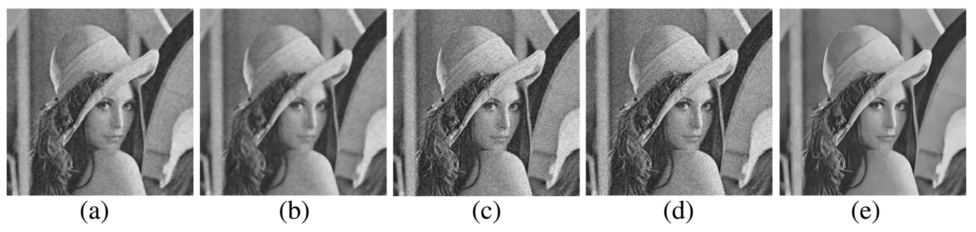
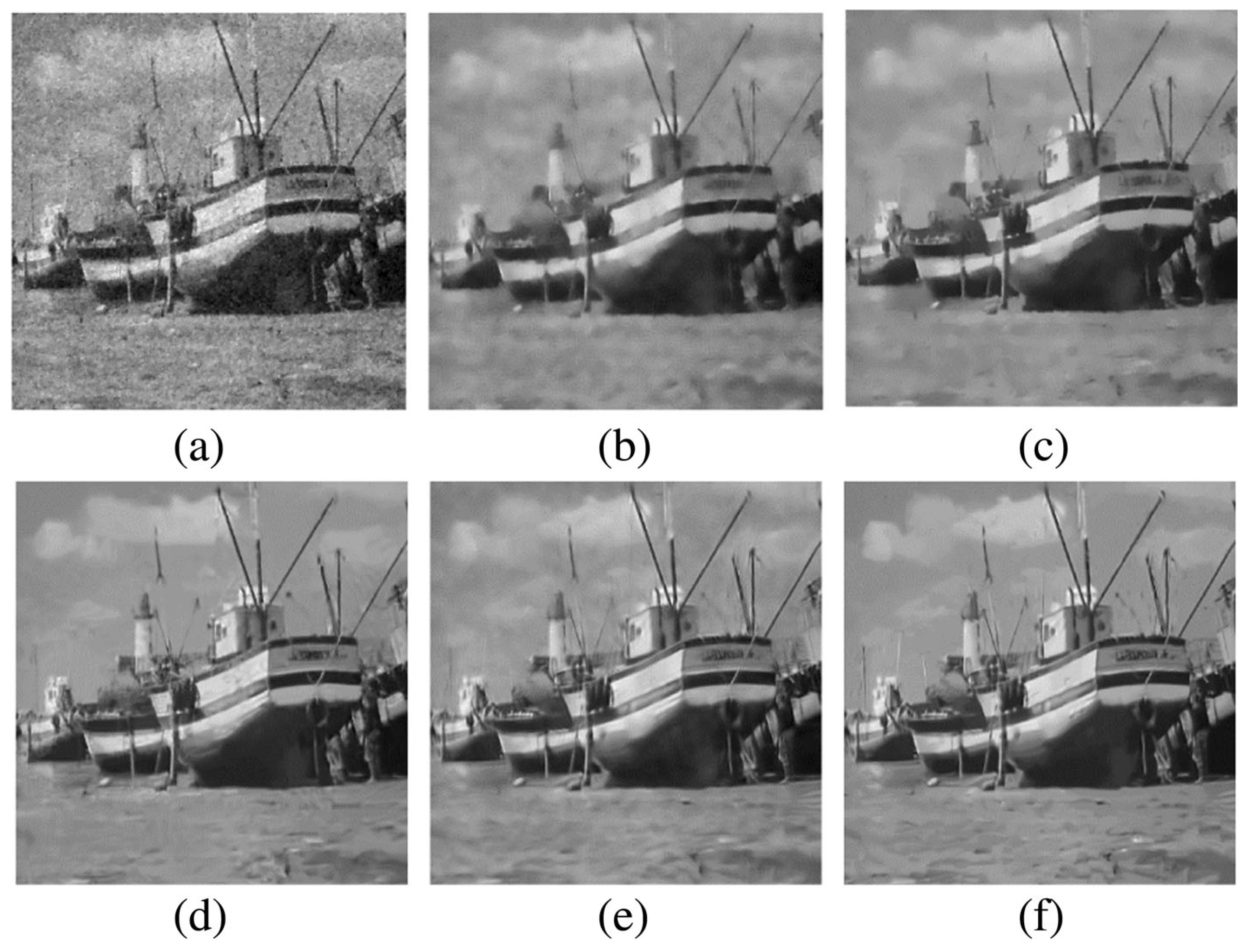
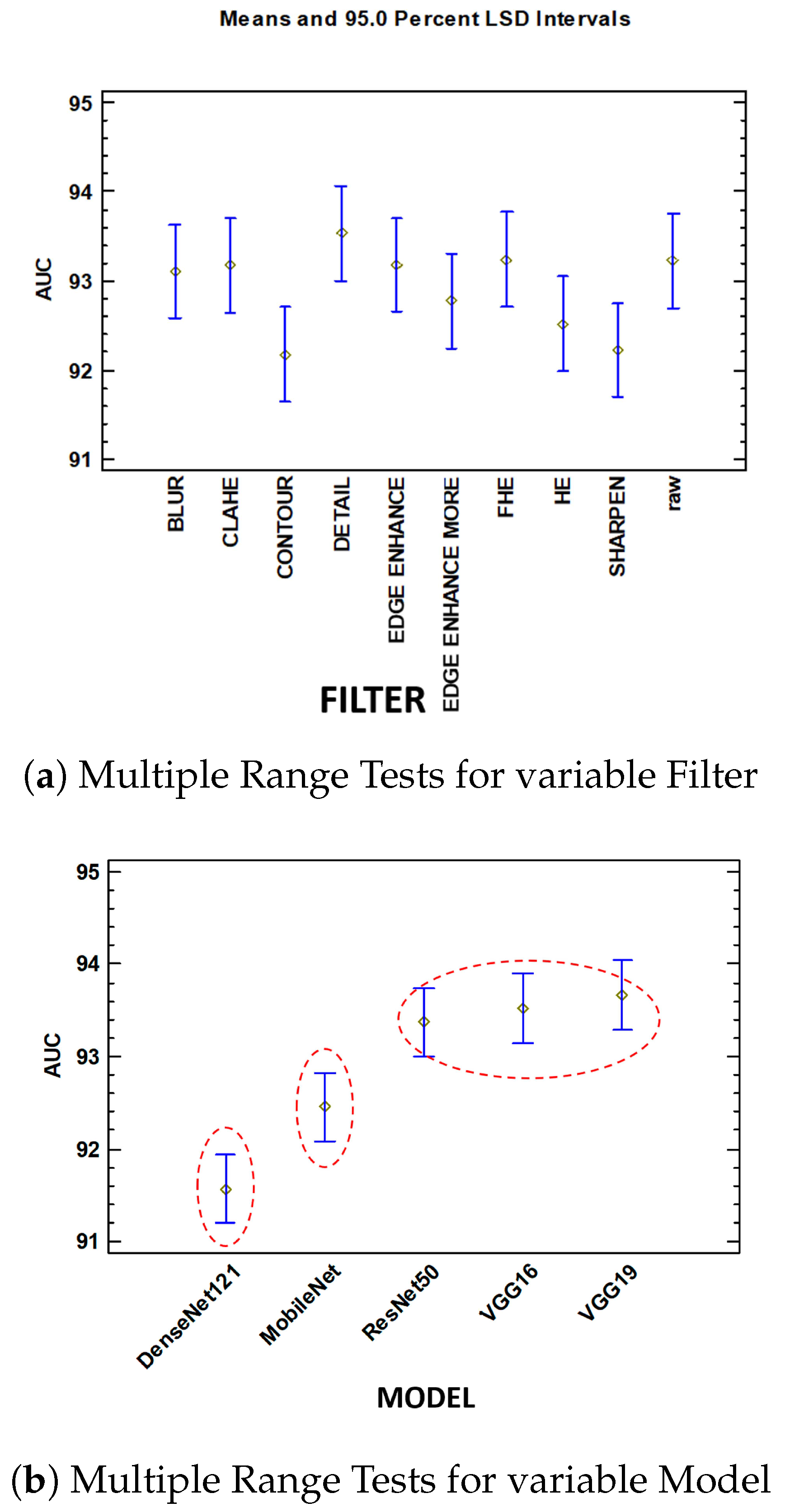
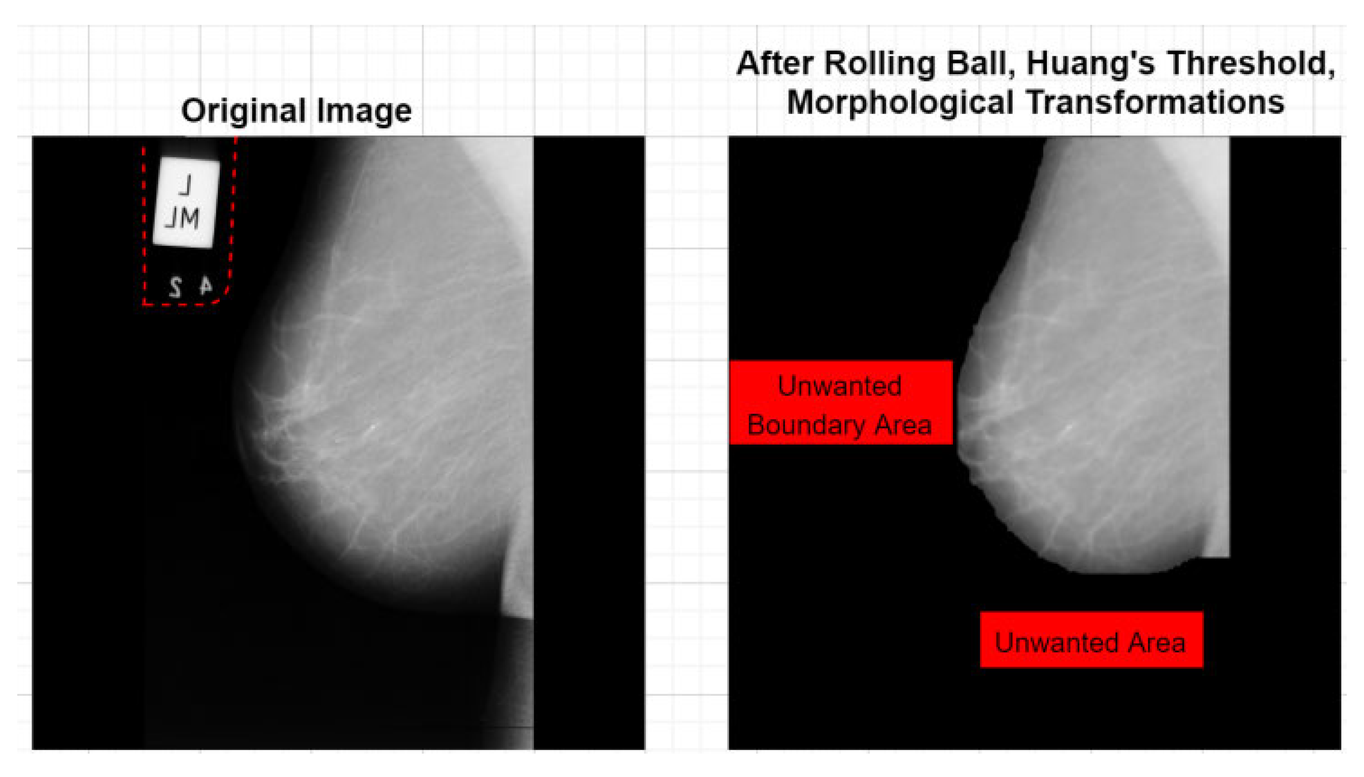
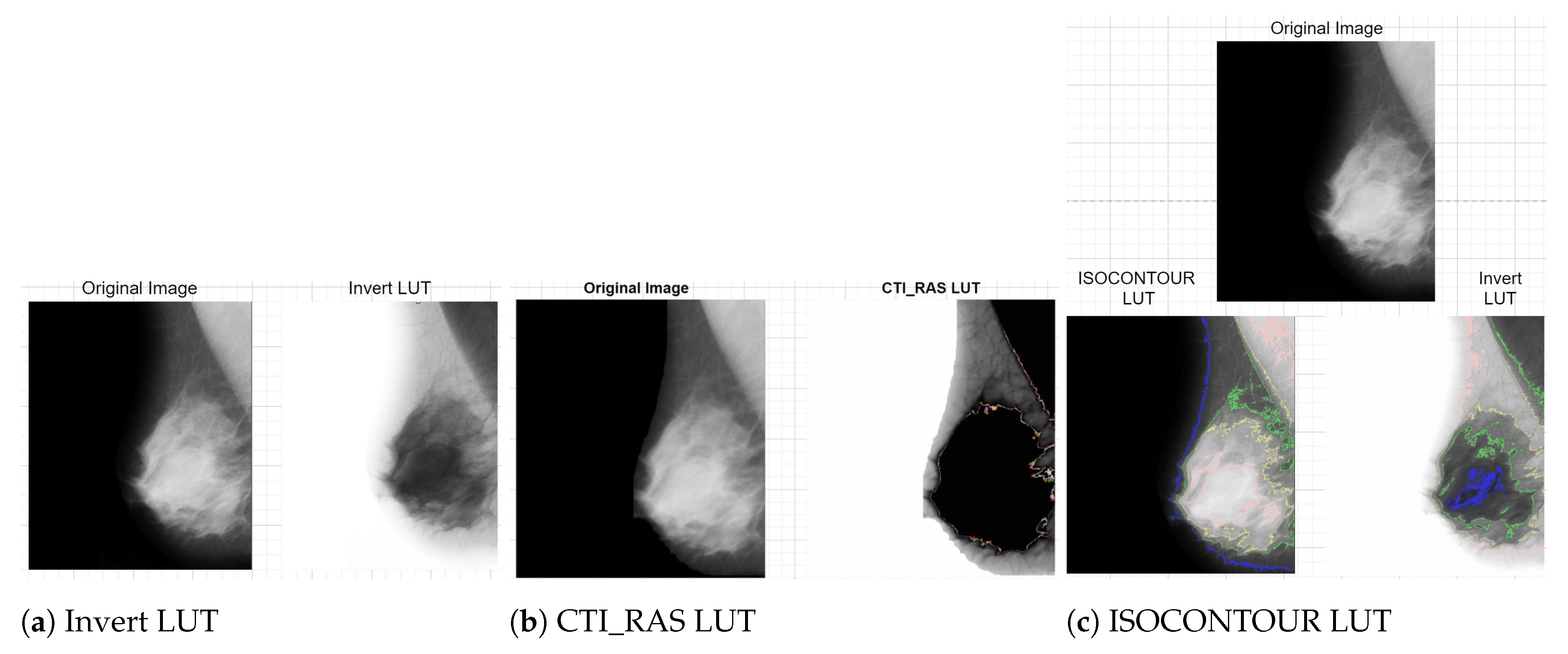
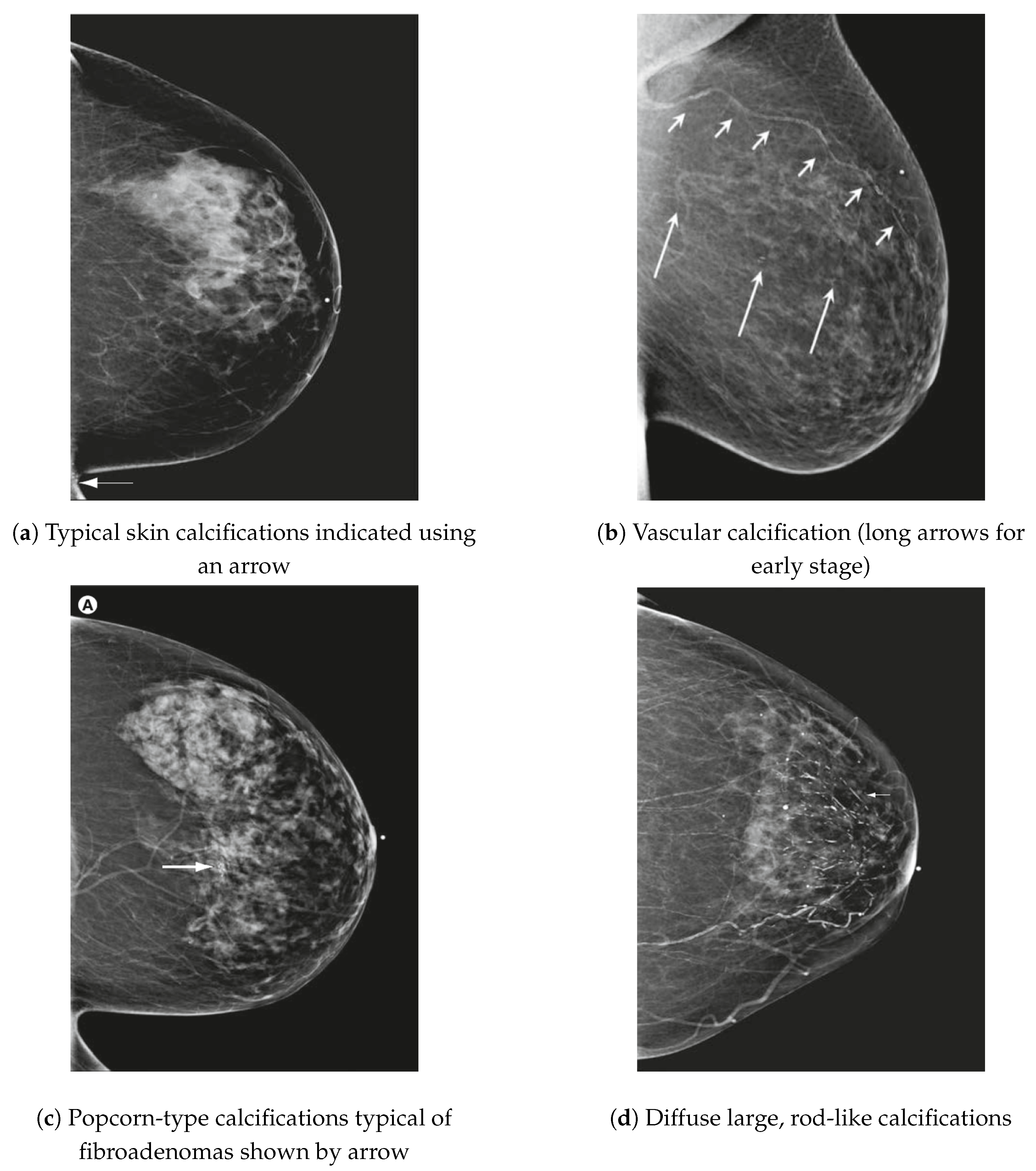
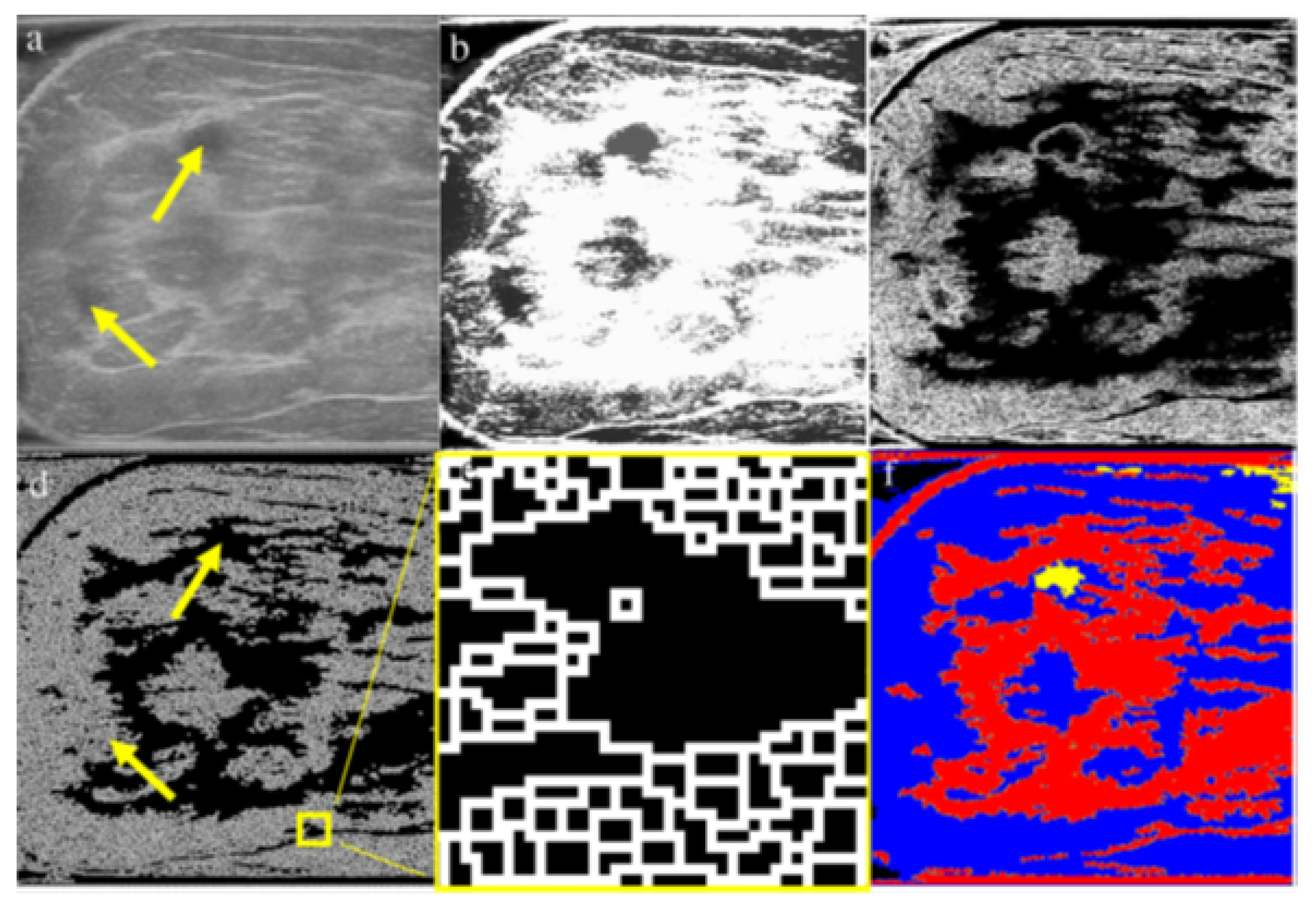
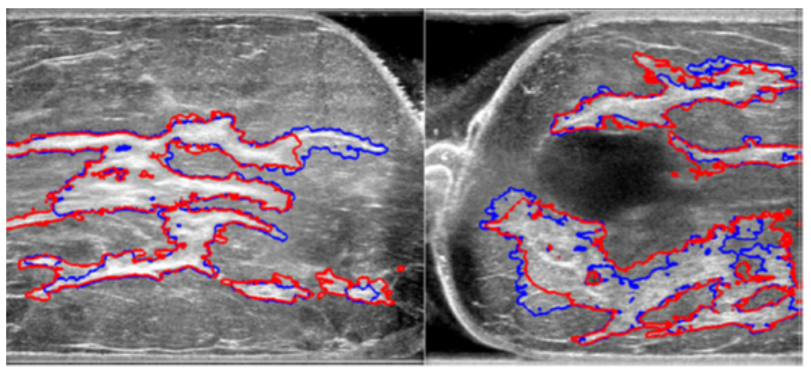
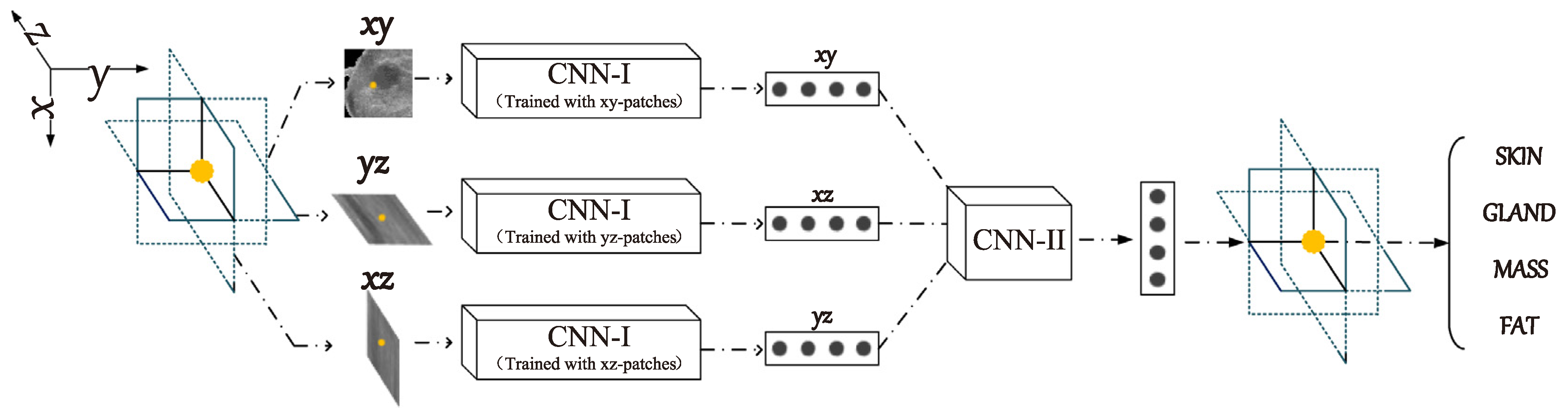
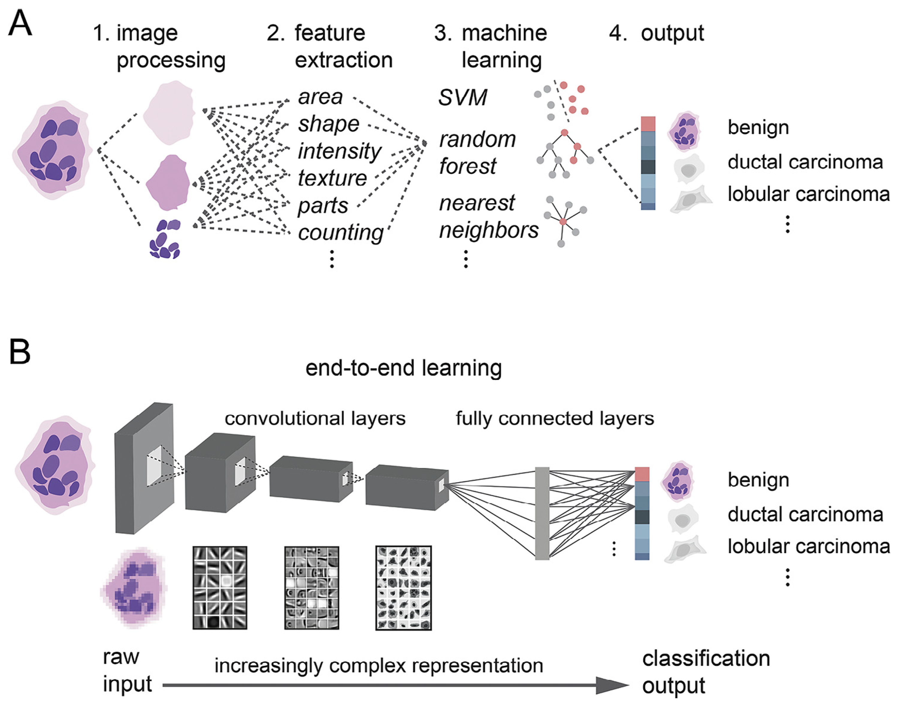
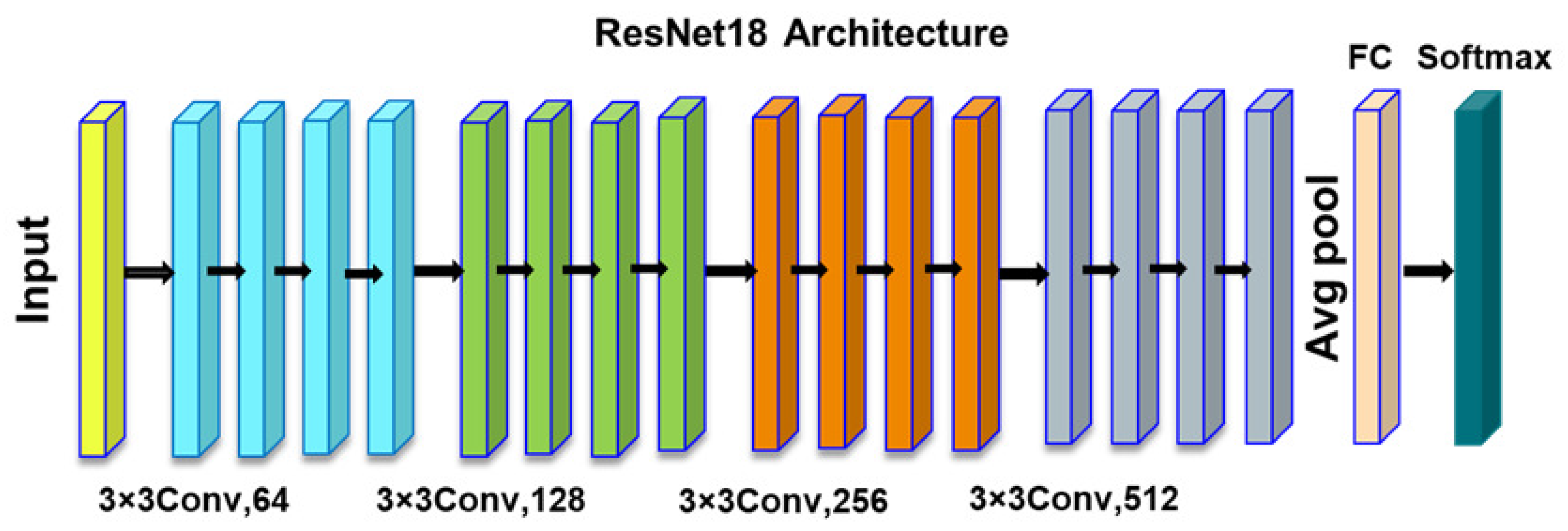
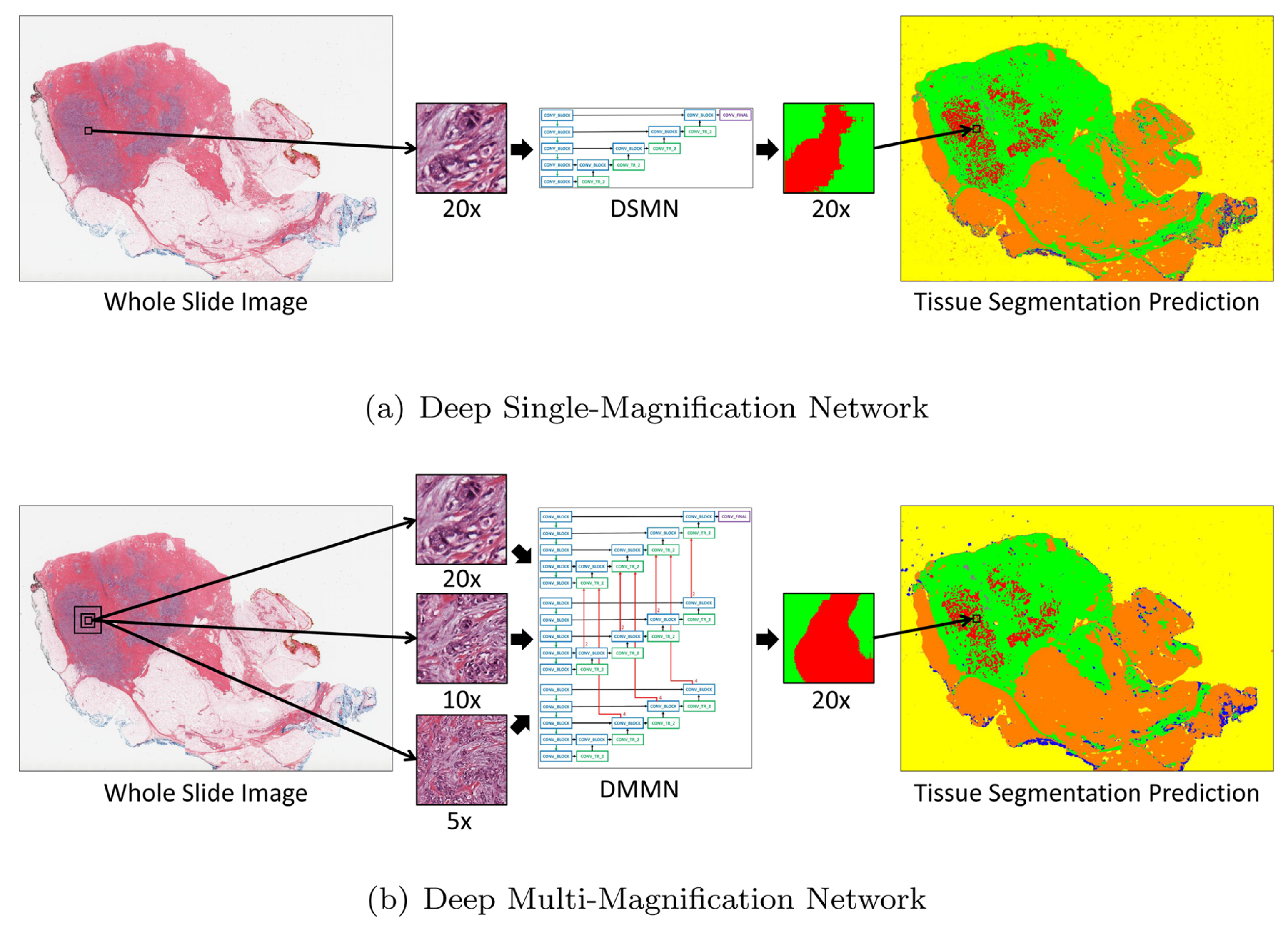


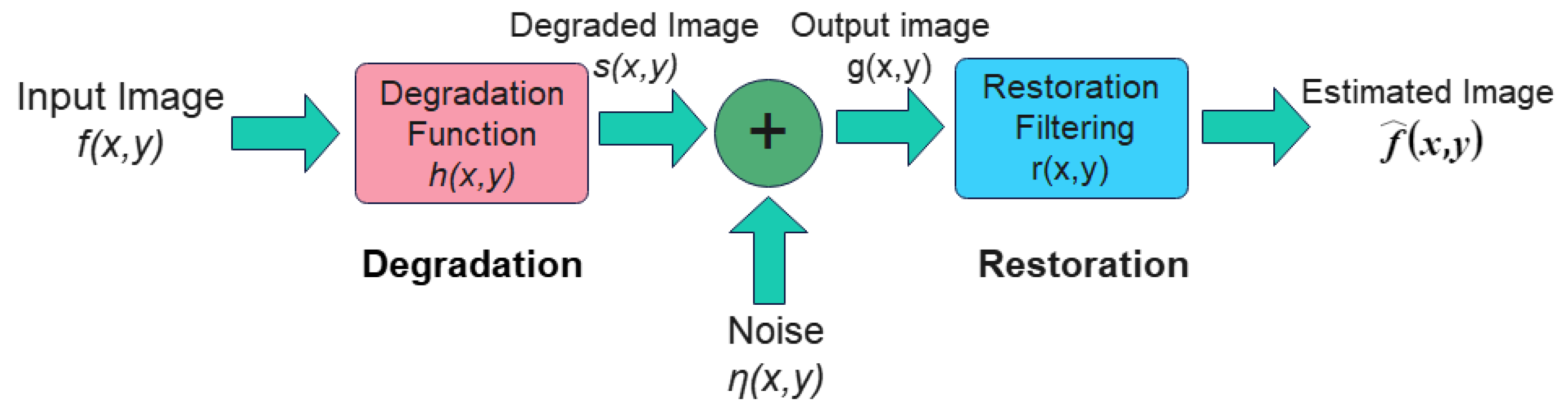
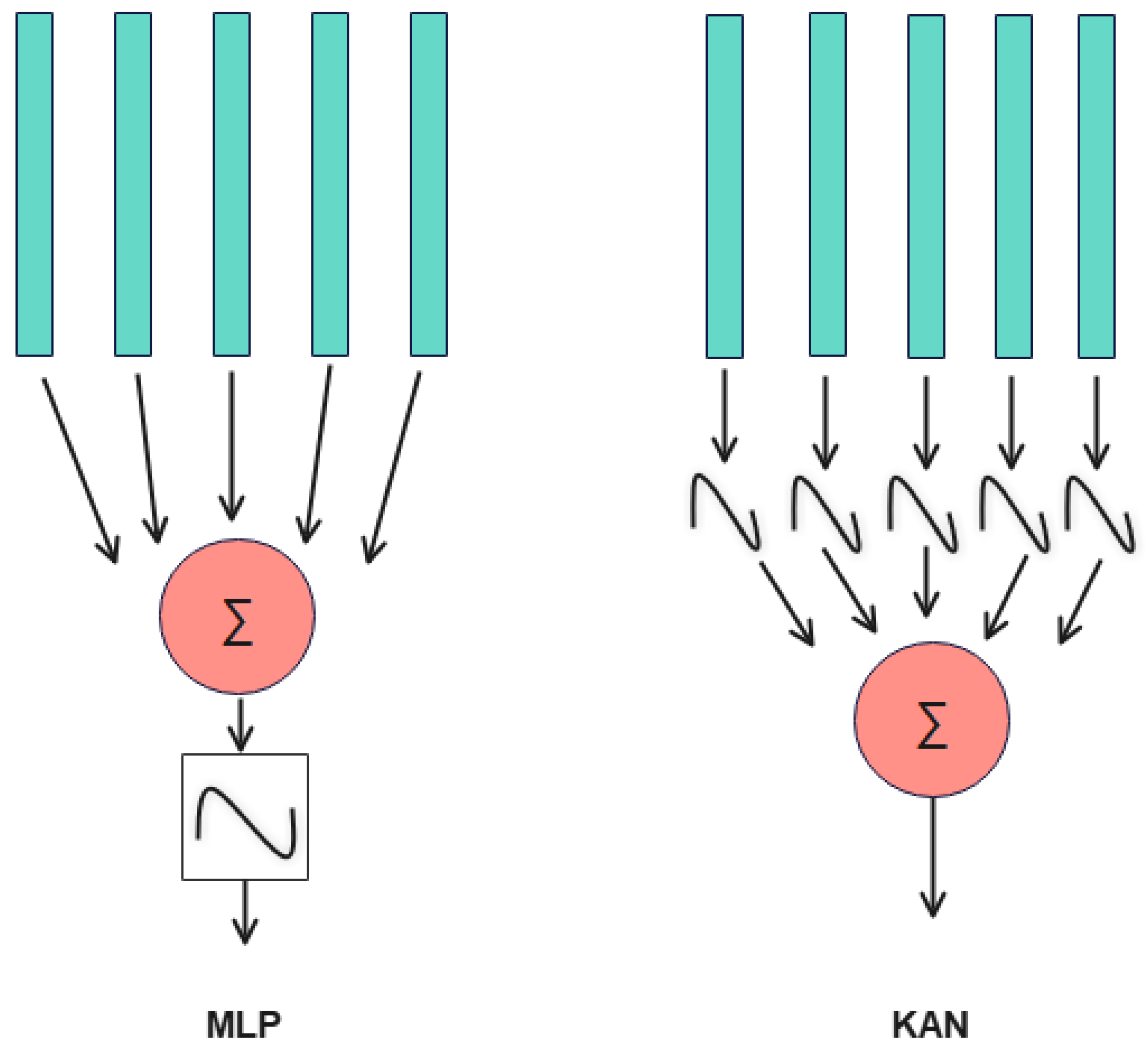
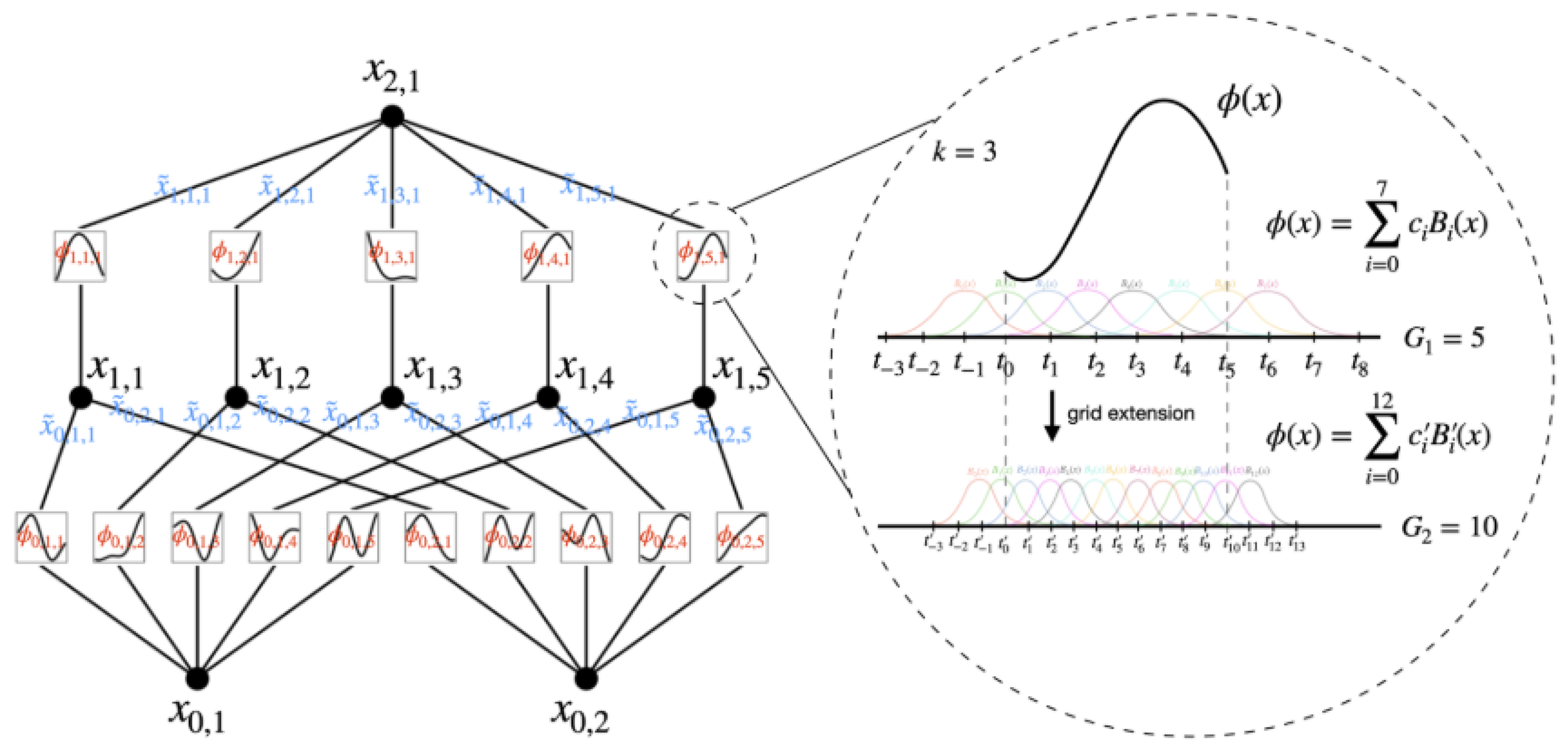
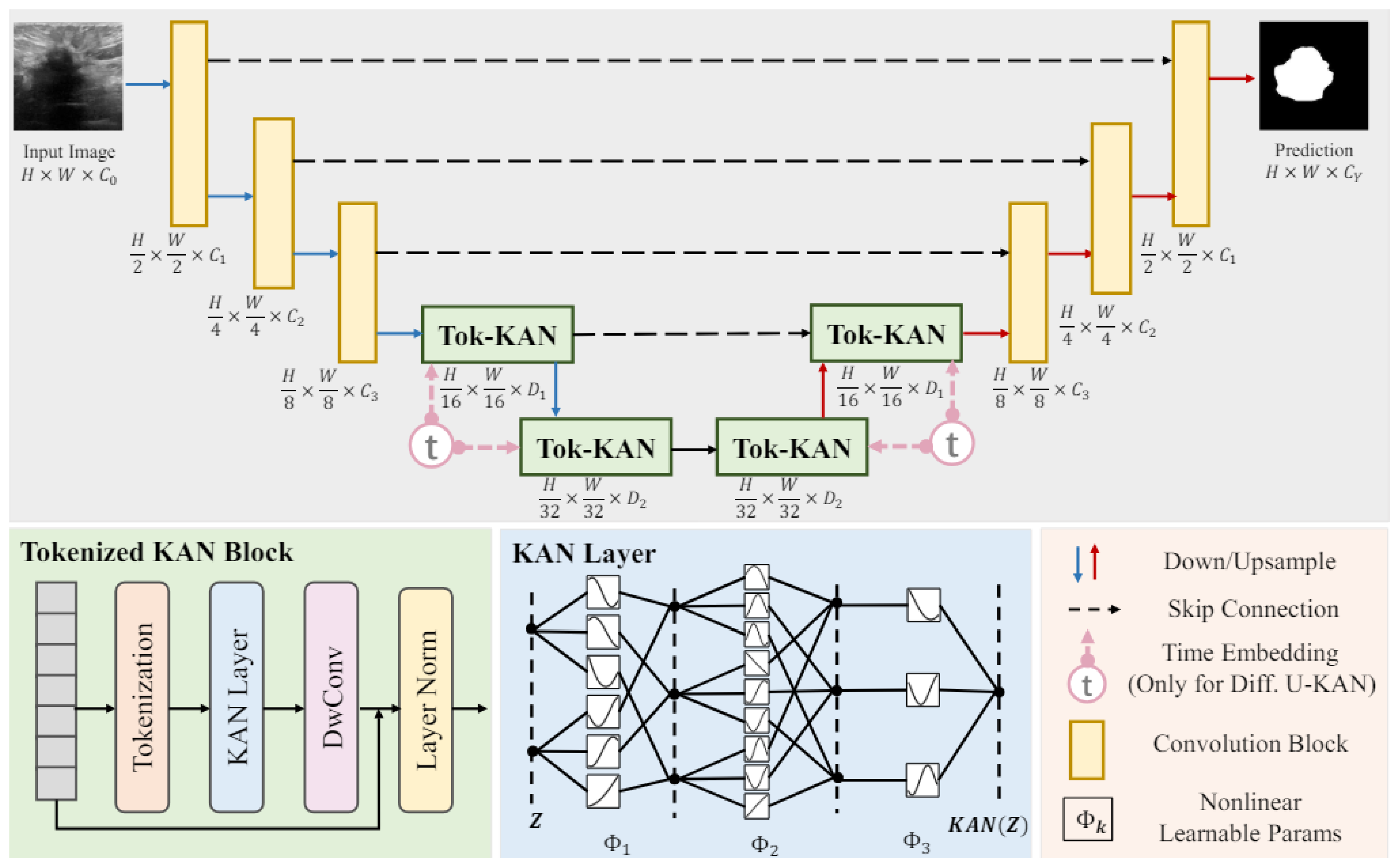
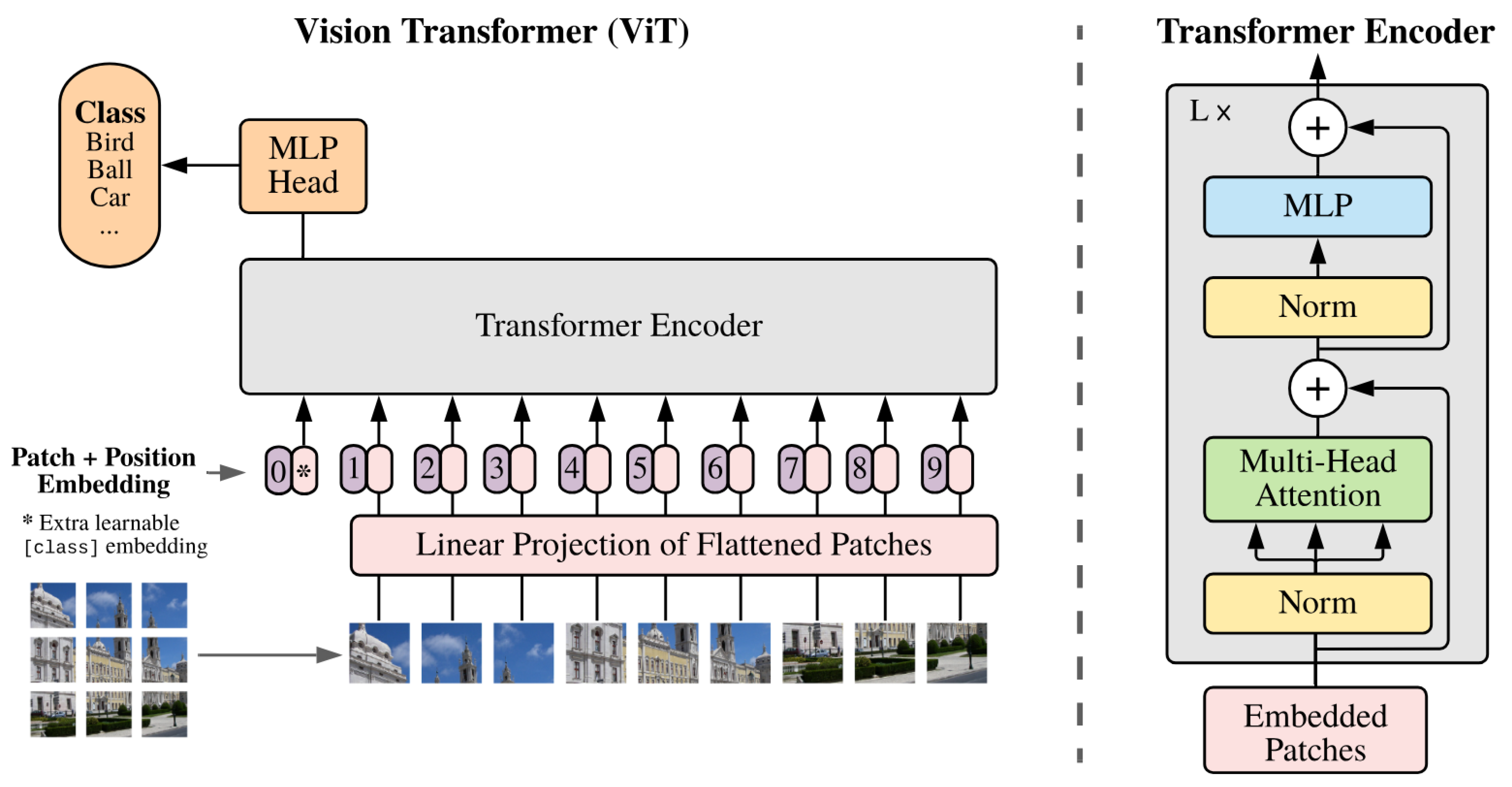
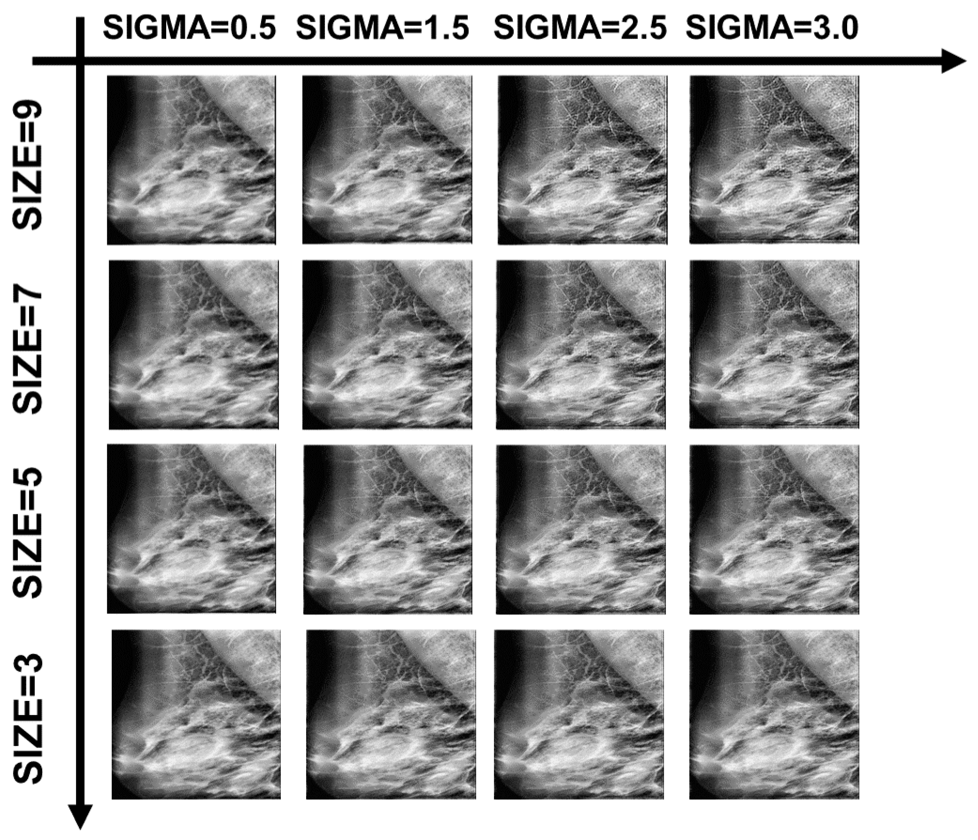
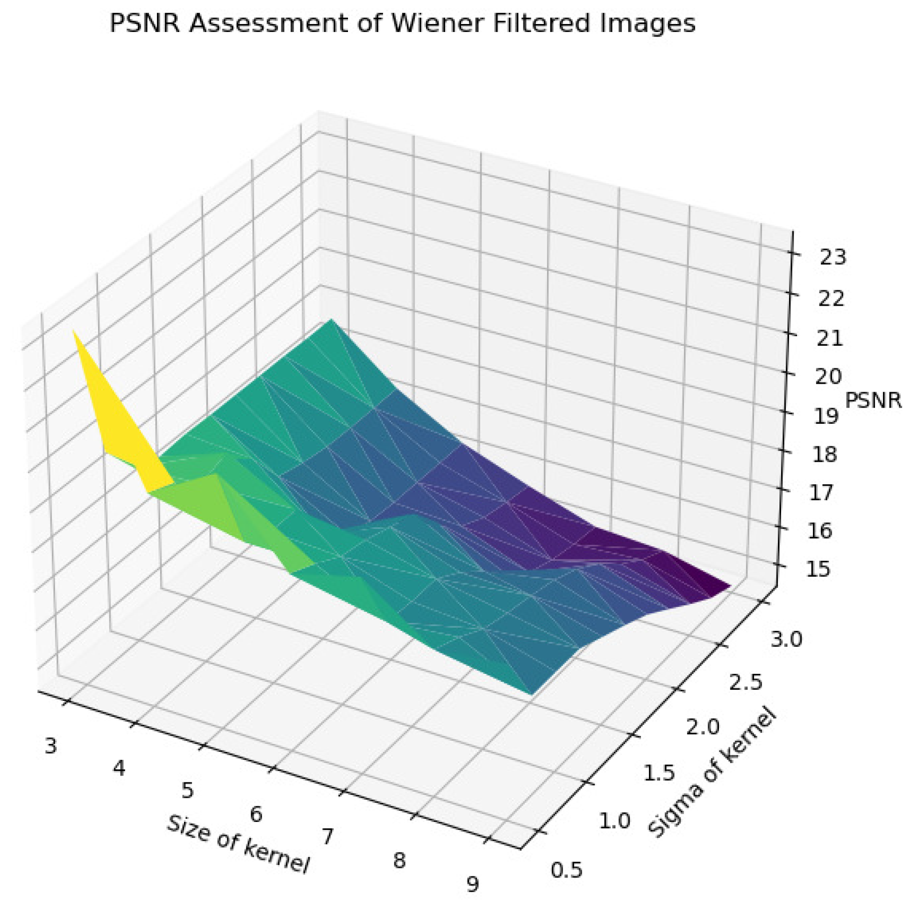

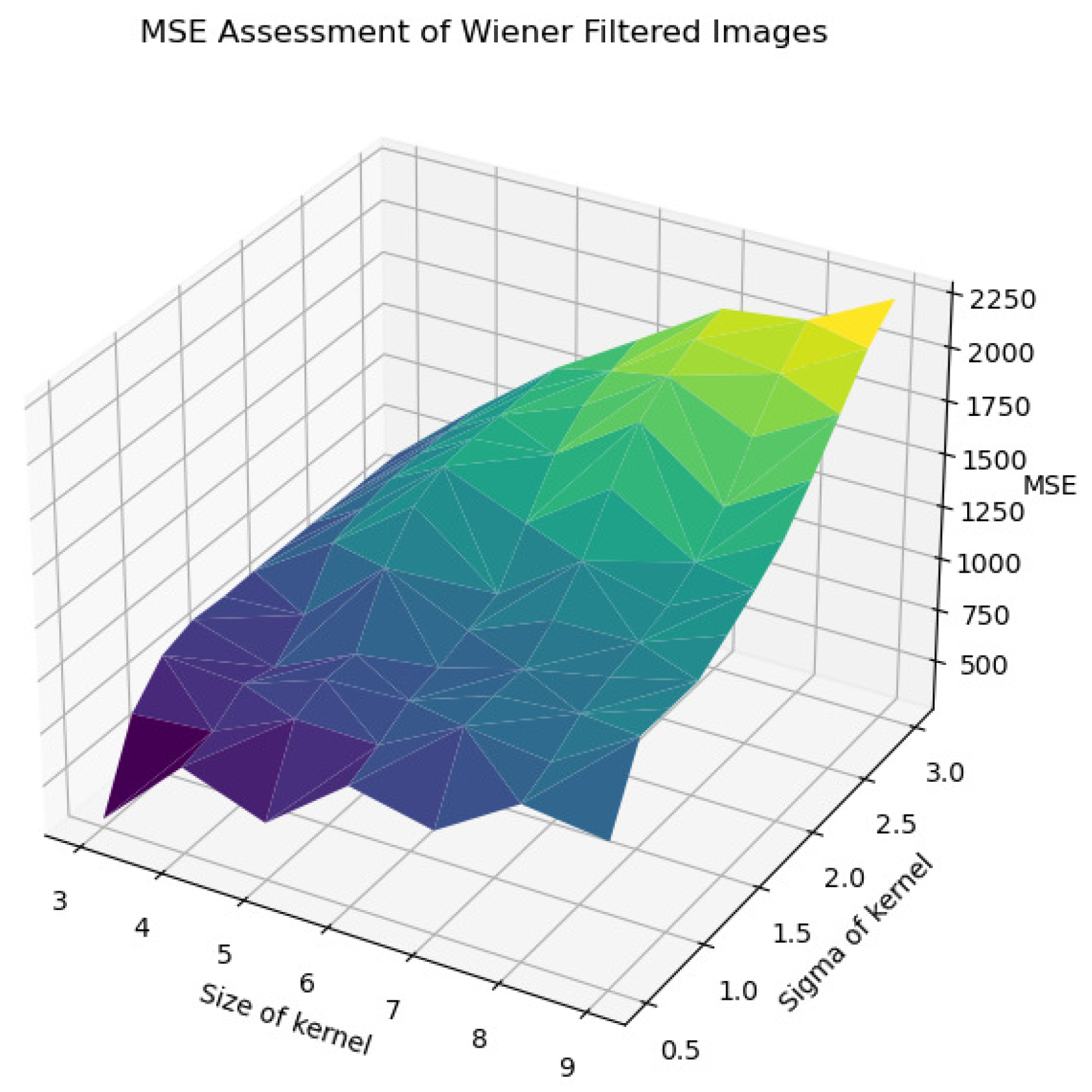


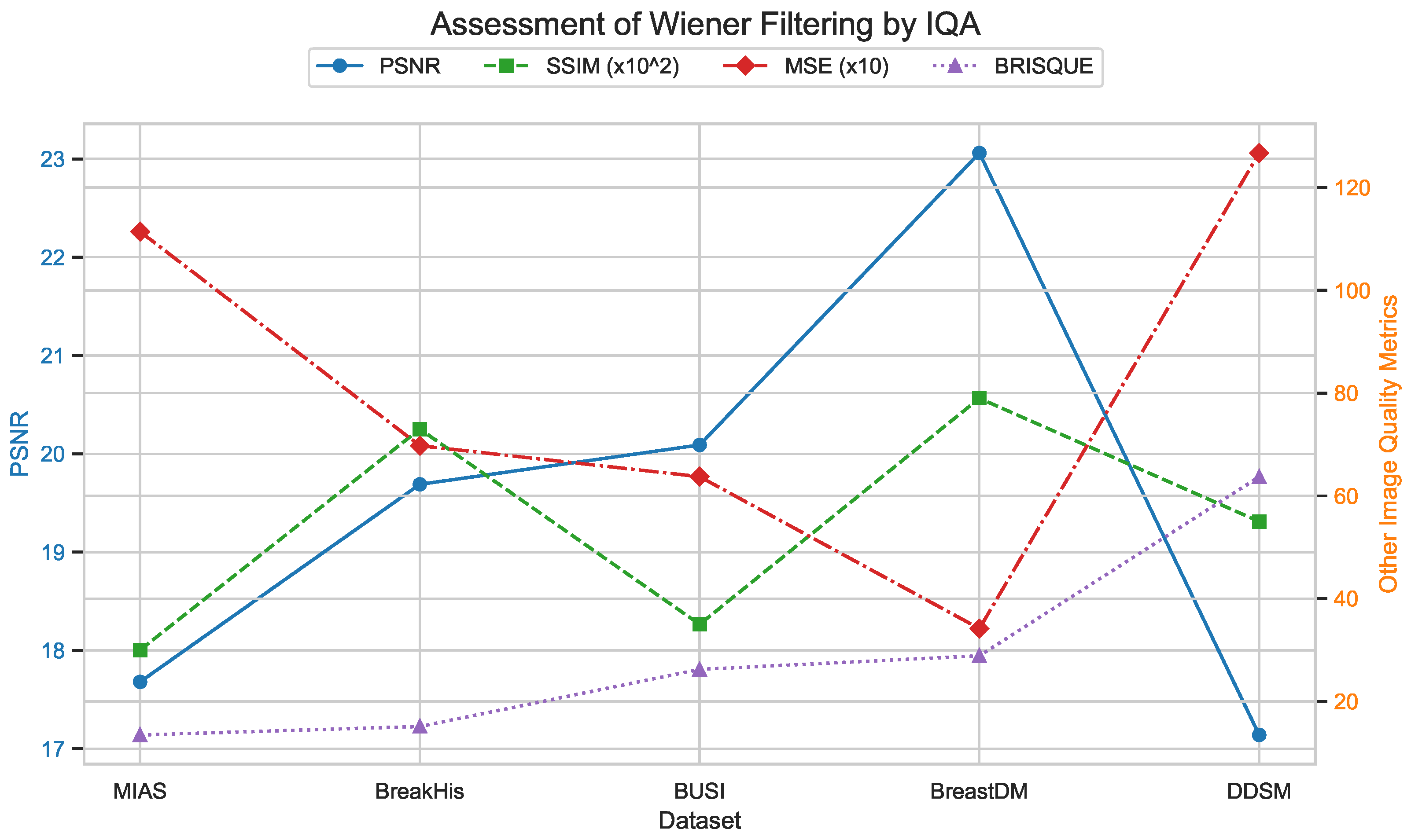
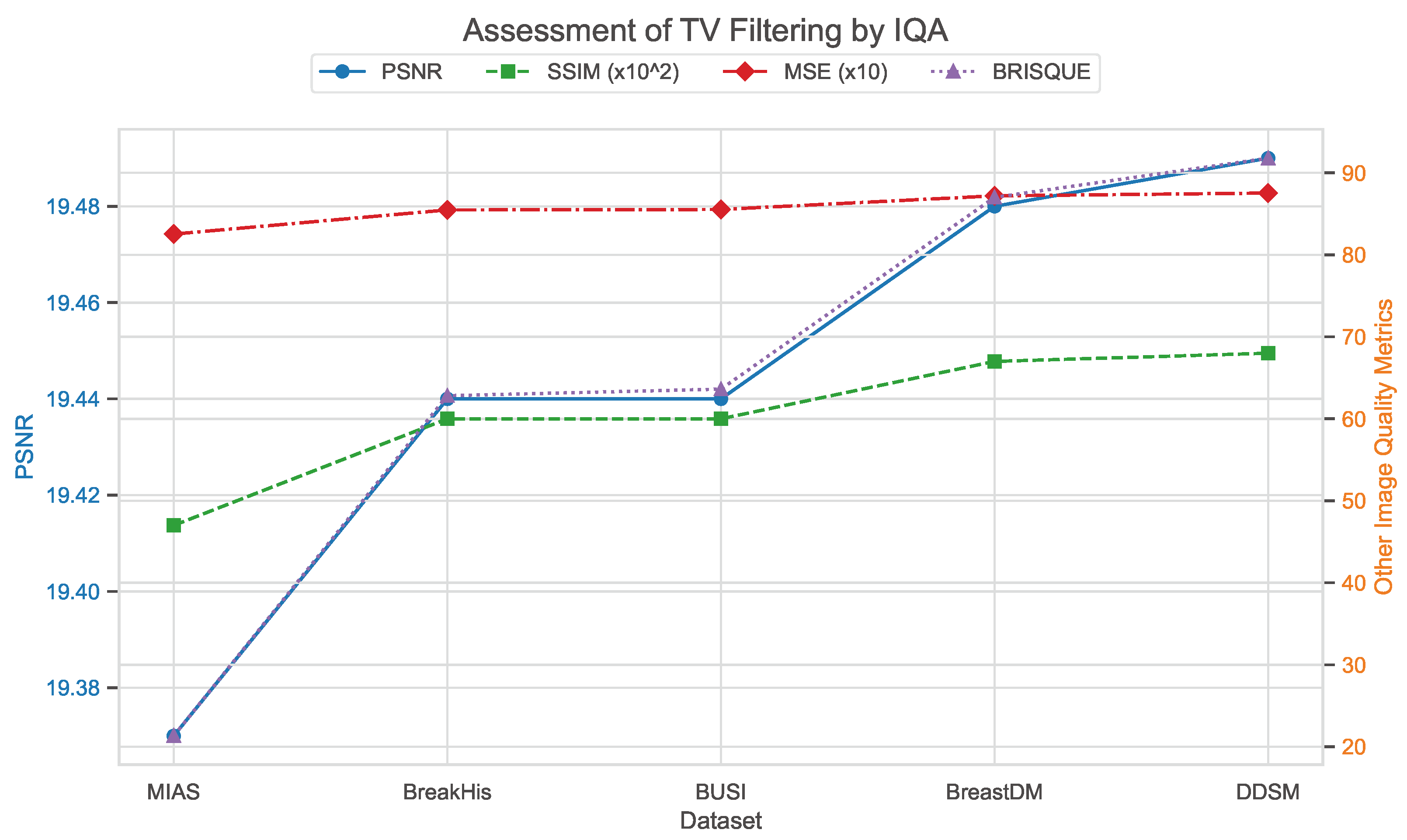
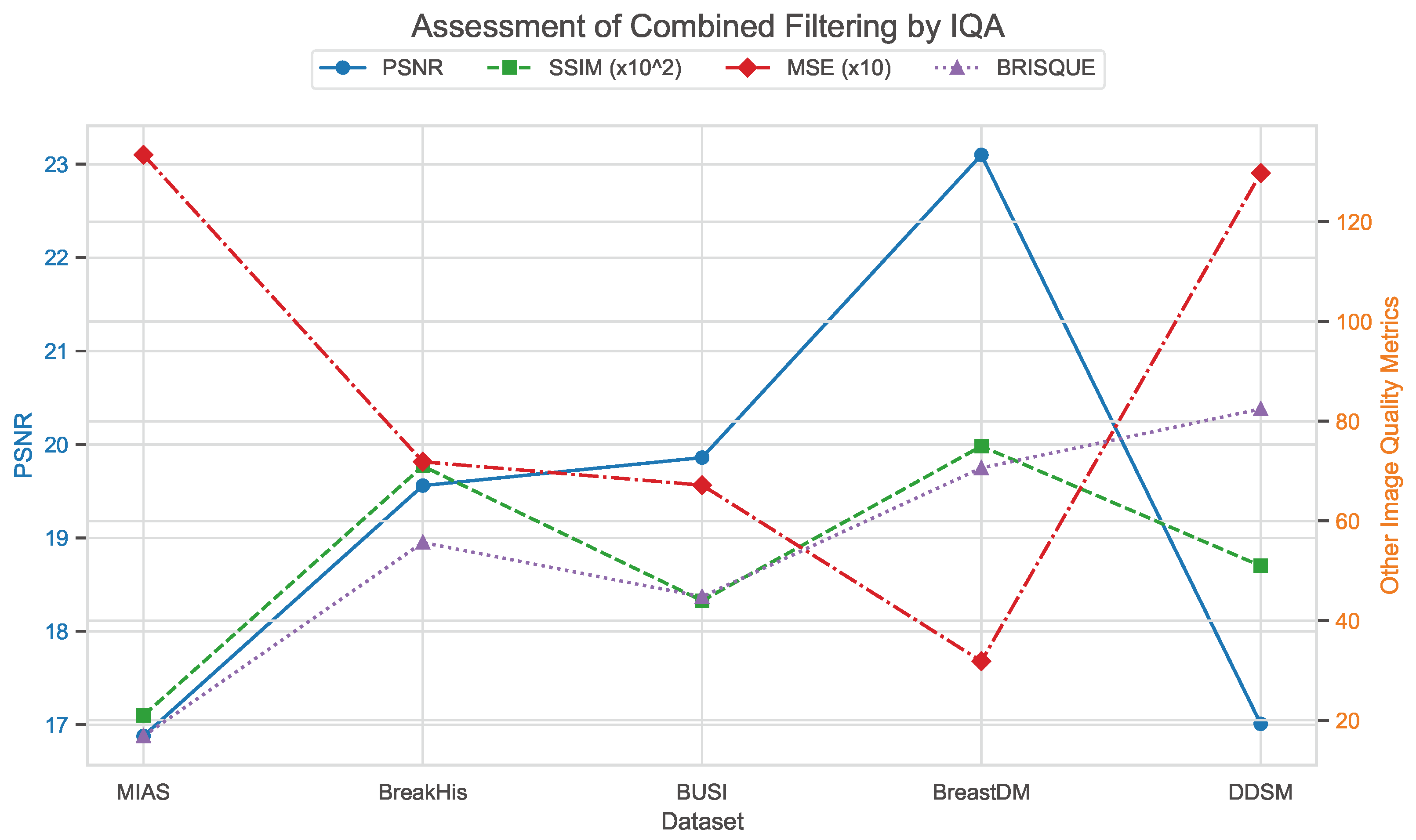
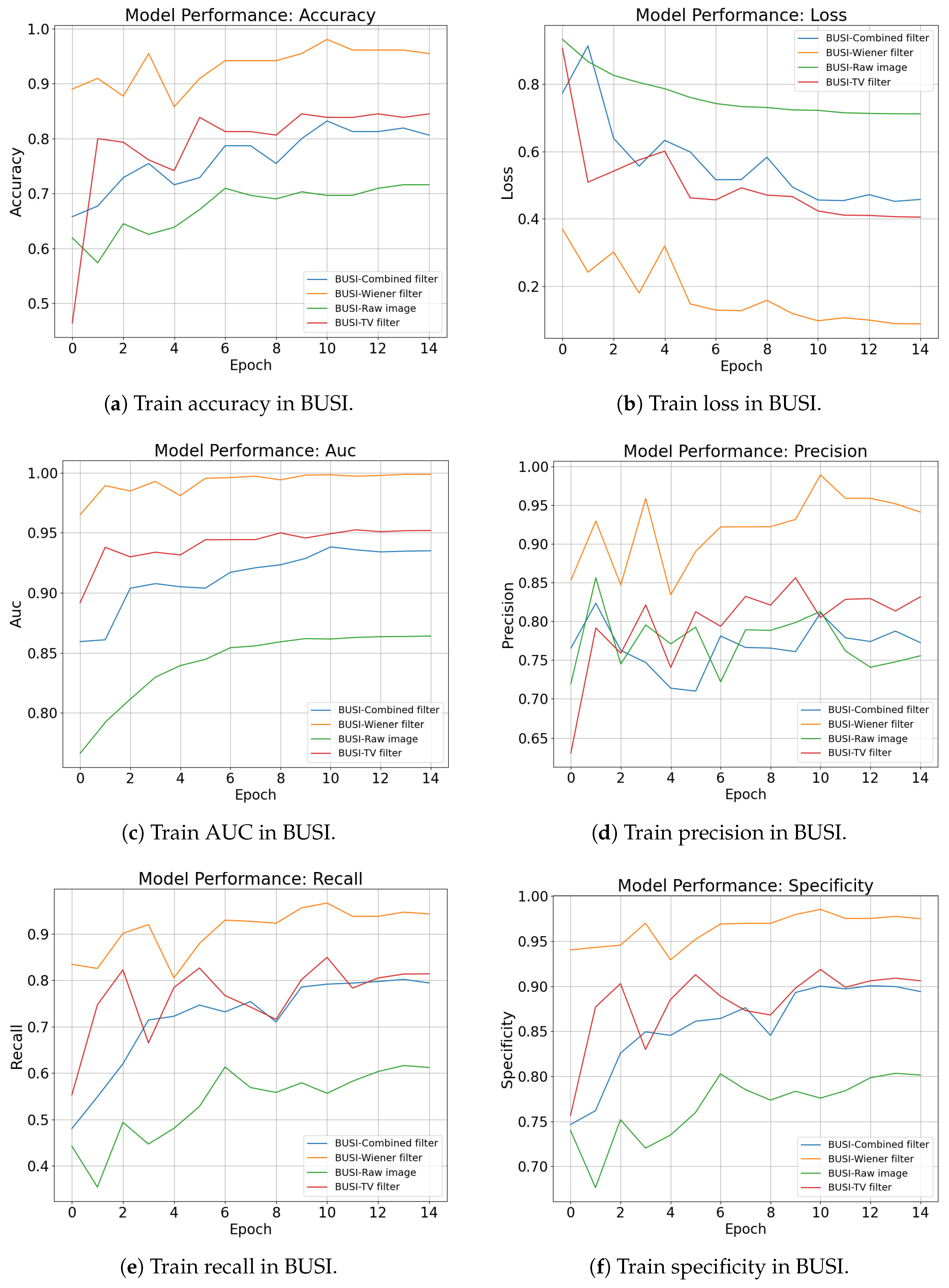
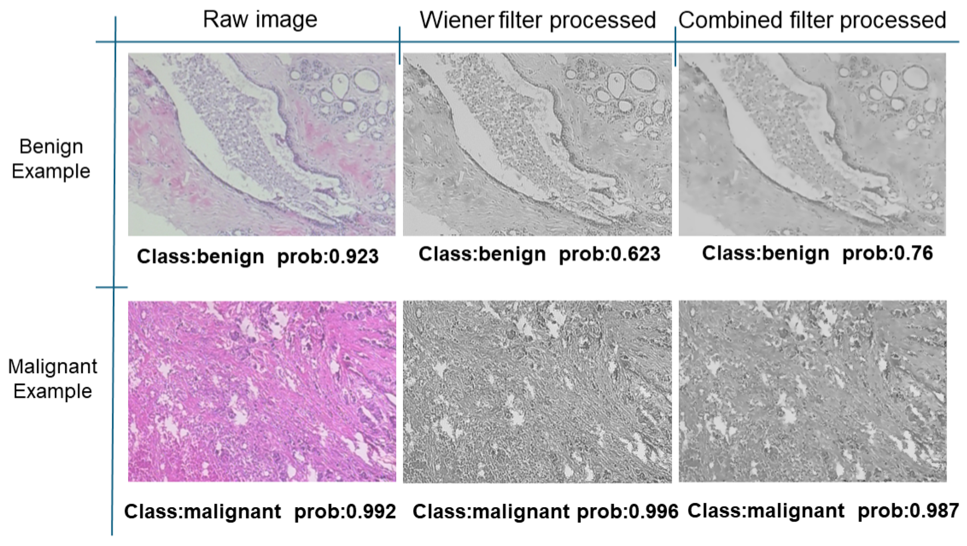
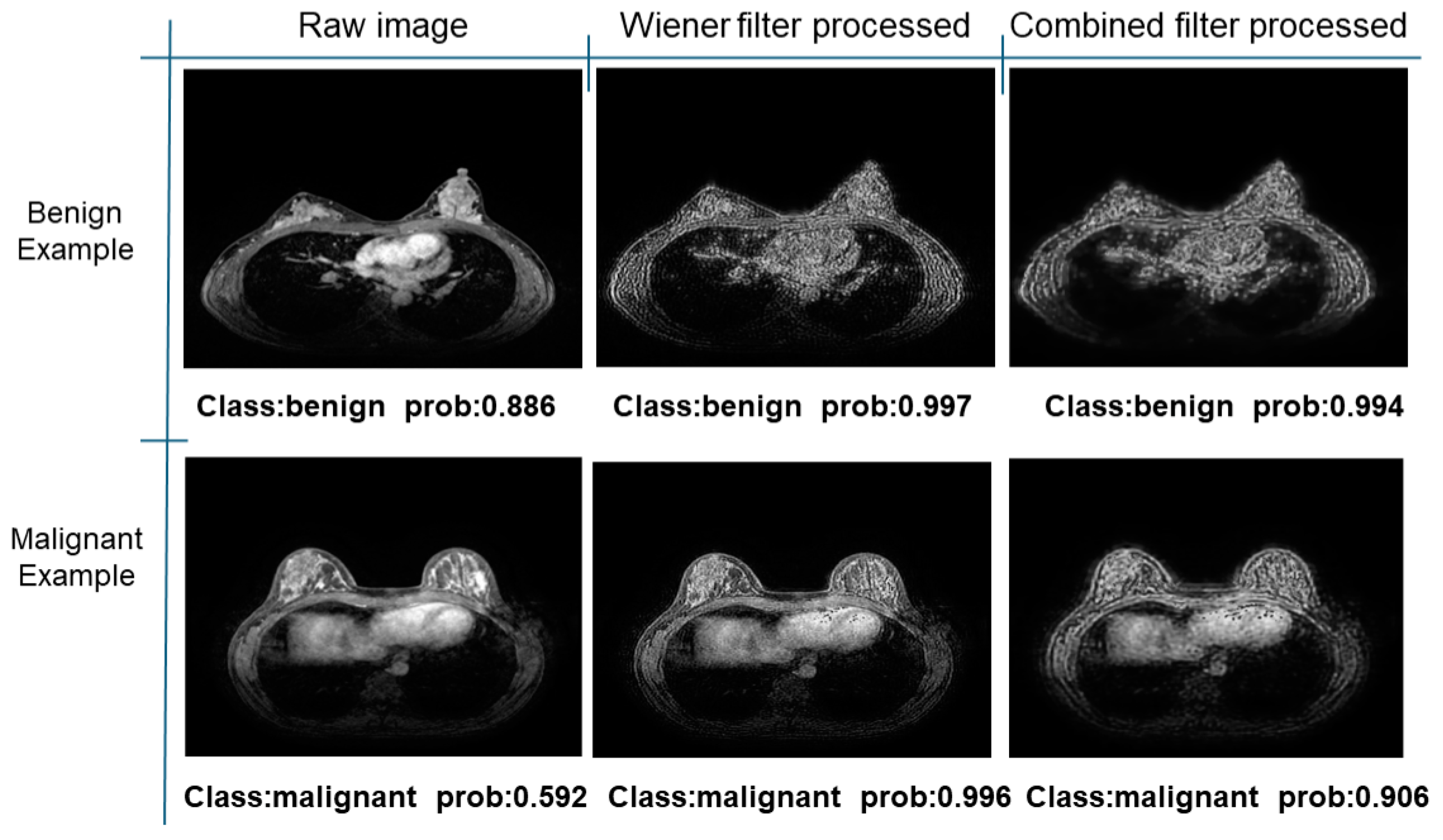
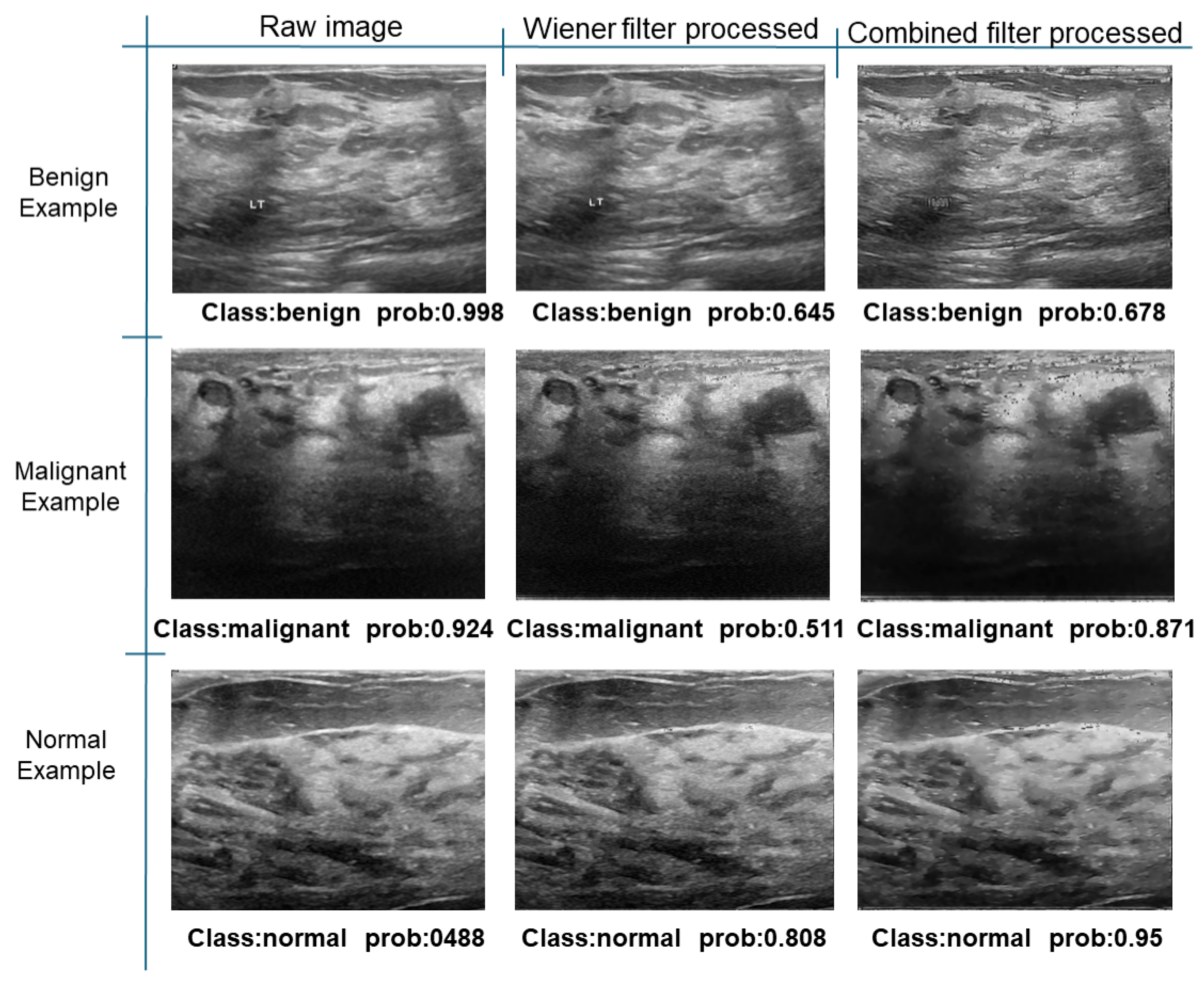
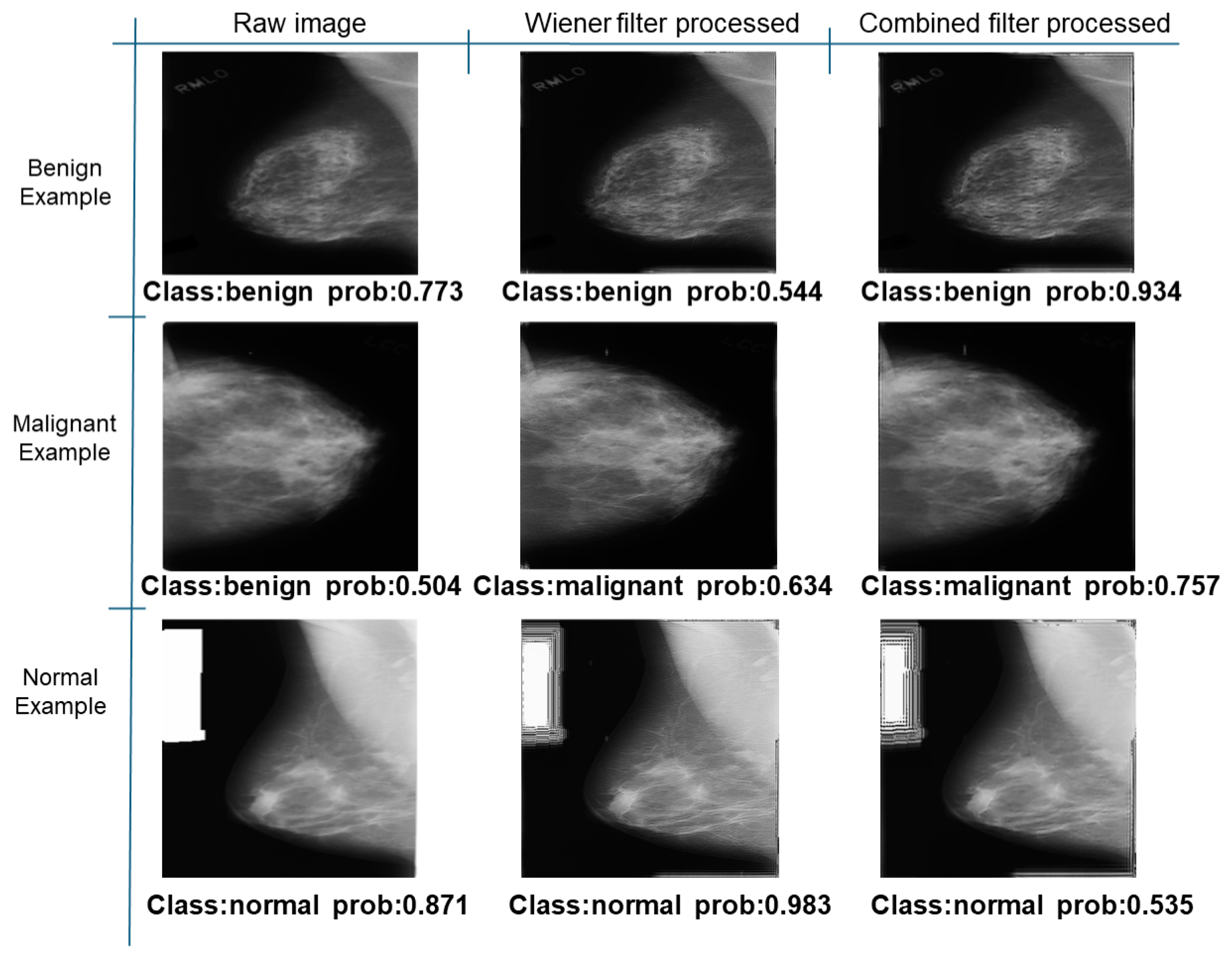
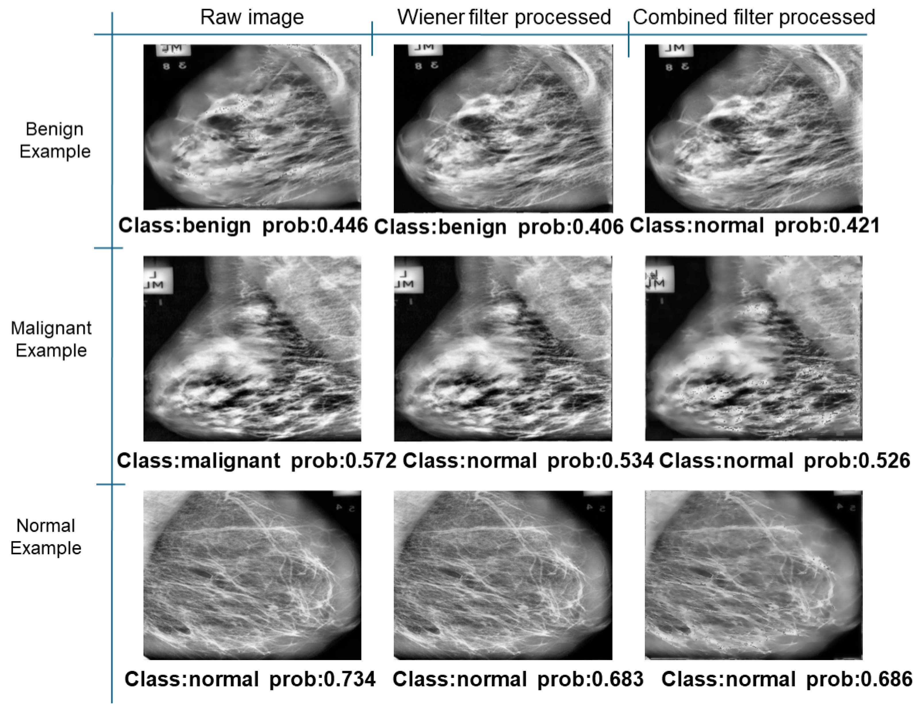
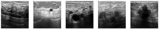
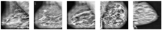
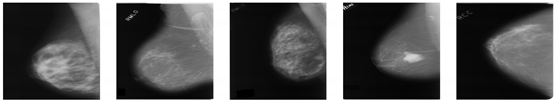
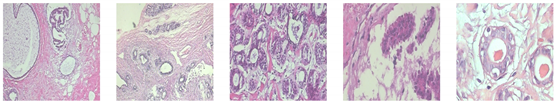
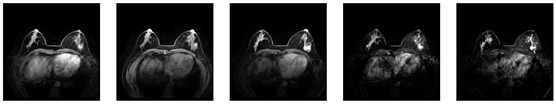
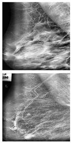


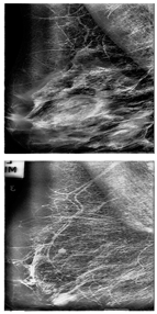
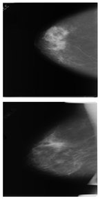
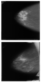
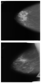
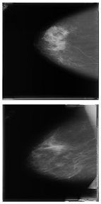
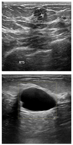
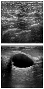
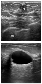
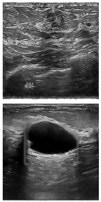
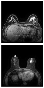

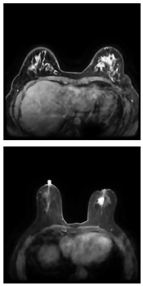
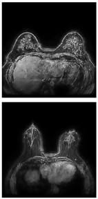
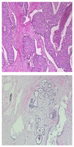
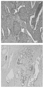

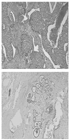


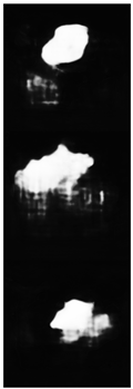
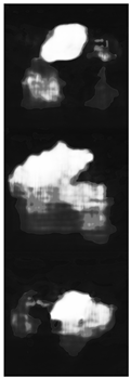

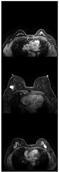

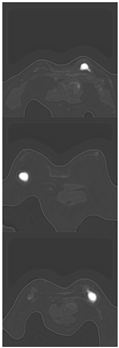
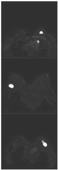

Disclaimer/Publisher’s Note: The statements, opinions and data contained in all publications are solely those of the individual author(s) and contributor(s) and not of MDPI and/or the editor(s). MDPI and/or the editor(s) disclaim responsibility for any injury to people or property resulting from any ideas, methods, instructions or products referred to in the content. |
© 2024 by the authors. Licensee MDPI, Basel, Switzerland. This article is an open access article distributed under the terms and conditions of the Creative Commons Attribution (CC BY) license (https://creativecommons.org/licenses/by/4.0/).