MLBSNet: Mutual Learning and Boosting Segmentation Network for RGB-D Salient Object Detection

Abstract

RGB-D saliency object detection (SOD) primarily segments the most salient objects from a given scene by fusing RGB images and depth maps. Due to the inherent noise in the original depth map, fusion failures may occur, leading to performance bottlenecks. To address this issue, this paper proposes a mutual learning and boosting segmentation network (MLBSNet) for RGB-D saliency object detection, which consists of a deep optimization module (DOM), a semantic alignment module (SAM), a cross-modal integration (CMI) module, and a separate reconstruct decoder (SRD). Specifically, the deep optimization module aims to obtain optimal depth information by learning the similarity between the original and predicted depth maps. To eliminate the uncertainty of single-modal neighboring features and capture the complementary features of multiple modalities, a semantic alignment module and a cross-modal integration module are introduced. Finally, a separate reconstruct decoder based on a multi-source feature integration mechanism is constructed to overcome the accuracy loss caused by segmentation. Through comparative experiments, our method outperforms 13 existing methods on five RGB-D datasets and achieves excellent performance on four evaluation metrics.

1. Introduction

Salient object detection (SOD) follows the human visual system to find the most visually appealing objects in a given scene. It has been widely used in many computer vision domains, such as visual tracking [1], image or video segmentation [2,3], face recognition [4], and person re-identification [5].

In recent years, SOD has relied on RGB images to achieve impressive results, but its performance is still limited by the use of single-modal information in certain extreme scenarios (such as low foreground–background contrast, extreme lighting conditions, background clutter, etc.). Unlike the color information provided by RGB, the spatial geometric cues provided by depth maps can help the network better segment the objects. So far, many approaches [6,7,8,9] have introduced depth information to SOD with encouraging results. However, current research methods often treat depth as the correct information to introduce into the network, often ignoring the effect of the inherent noise of the depth map.

First, some processing schemes made for depth maps have been proposed in several works of literature [10,11,12]. Among them, Fan et al. [13] proposed a filtering scheme to screen the depth maps. Ji et al. [11] avoided the effects of low-quality depth maps by giving them lower weights. To improve the quality of low-quality depth maps, Chen et al. [14] supplemented the original depth information by estimating additional high-quality depth information to improve detection performance. At the same time, all these methods take complex preprocessing operations for depth maps. Given the small amount of data, discarding low-quality depth maps or giving lower weights to low-quality depth maps may not always achieve the desired purpose. In [15], utilizing the predicted depth maps in RGB after subsequent fusion greatly improved the performance of the model. Thus, the predicted depth maps can provide useful clues. Inspired by this, we plan a mutual information minimization depth map scheme to alleviate the effects of unstable depth maps. In this work, we employ an end-to-end network to obtain predicted depth maps. To explore the relationship between the predicted depth map and the original depth map, we first combine the two to obtain maximum information and then learn from each other with the original and predicted depth map to obtain more stable depth maps. At the same time, to maximize the accuracy of the predicted depth maps, we constrain them using similarity loss. As shown in Figure 1, our proposed model can work well for those unreliable depth images compared to other models for depth map correction.

Figure 1. Visualization of significance maps in the case of unstable depth maps: (a) RGB, (b) depth, (c) GT, (d) ours, (e) DCF [11], (f) D3Net [13], and (g) DSANet [15].

Secondly, we further consider the issue of modal alignment before fusing the features. In previous works, many approaches are more biased towards considering cross layers of fused feature alignment in the decoder part. However, the network’s feature extraction process makes features at neighboring levels differ in detail while being extremely correlated in terms of abstract semantic information. While existing methods [16,17] directly knead and sum the features of each layer and then put them into the subsequent decoder for feature extraction. As a result, this approach tends to ignore intermodal matching incompatibilities. To overcome the above limitations, we propose a semantic alignment program to reduce the variability and enhance the correlation between neighboring features by employing a graph attention mechanism. Then, to integrate complementary fusion information between RGB images and depth maps, we propose a self-attention fusion scheme to learn more common representations of both.

Finally, we believe that the segmentation structure of the network very much affects the performance of the model. Most models [18,19,20] use a U-shaped network structure to integrate fused features and segment target objects. While this top-down approach is powerful in integrating multilevel features and context awareness, the incremental stacking of features may lead to redundant information and not utilize the full potential of fused features. To this end, we propose a novel framework for the separation–reconstruction decoder. Firstly, we separate the fusion features equally and then reintegrate the separated fusion features, different levels of RGB features, and depth features in the multi-source information integration module for reconstruction. On the one hand, we retain the original fusion information and avoid information loss caused by up-sampling. On the other hand, the learning of information between different input sources allows the network to learn more discriminative features.

In summary, our main contributions can be summarized as follows:

• We propose a mutual learning and boost segmentation network (MLBSNet) that completes the deep optimization, feature fusion, and information inference process through the deep prediction and saliency goal inference stages. The five RGB-D SOD datasets yield excellent experimental results and outperform the state-of-the-art models.
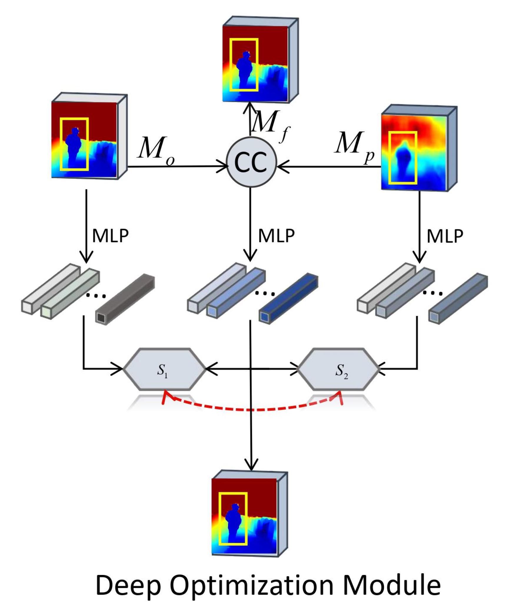
• We introduce a deep optimization module (DOM) to obtain more accurate depth information through similarity learning, which provides more effective complementary features for fusion.
• We designed the semantic alignment module (SAM) with a graph attention mechanism to eliminate the variability between the neighboring features of a single modality. The output features are then fed into a cross-modal integration (CMI) module to collect cross-modal complementary information.
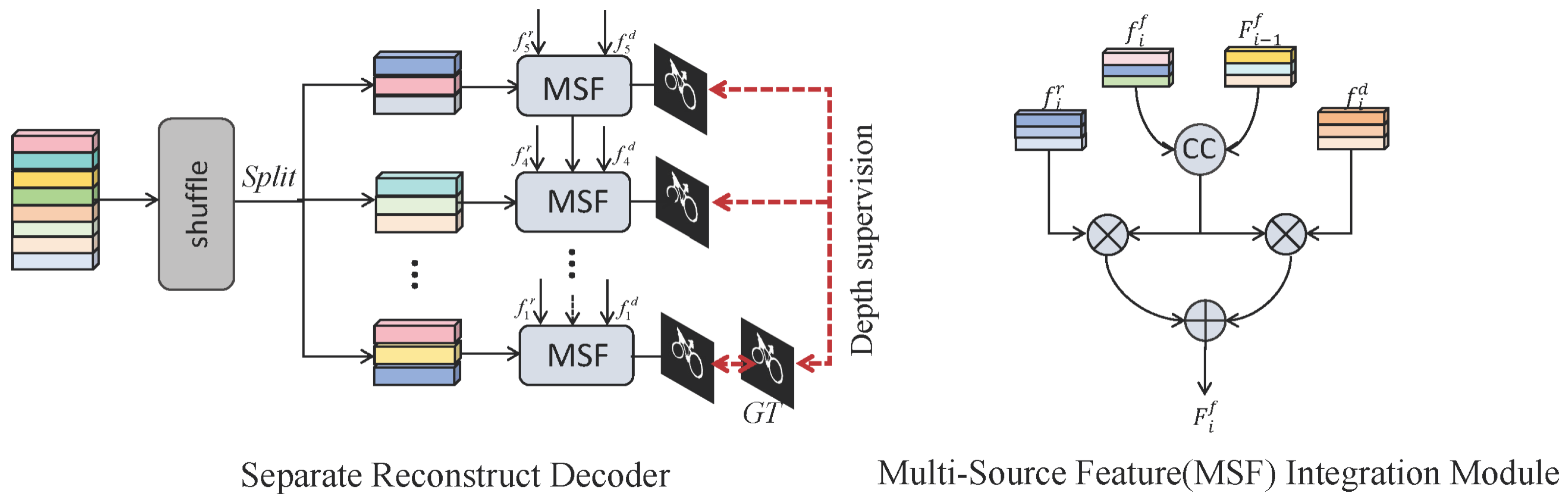
• We build a simple and effective separate–reconstruct decoder (SRD) that not only avoids information loss caused by up-sample but also integrates rich multi-source features.

2. Related Work

RGB-D Salient Object Detection

Early RGB-D SOD accomplished the task mainly through traditional handcrafted features (e.g., prior [13], contrast [21], and shapes [22]). However, limited by the handcrafted feature representation capability, these methods may not achieve satisfactory results. Recently, with the development of deep learning, benefiting from its powerful feature representation, CNN-based RGB-D SOD methods [23,24,25] have achieved satisfactory results. Currently, RGB-D SOD methods are divided into three main categories: early fusion [26,27], resultant fusion [28], and cross-level fusion [29,30]. Among them, cross-level fusion has become the mainstream method in recent years.

These RGB-D SOD methods based on cross-level fusion mainly accomplish saliency object detection by fusing complementary information between RGB images and depth maps. Sun et al. [31] proposed a cascaded aggregated transformer network, which is used to enhance RGB features and depth features that mitigate the interference of low-quality depth maps in the encoder stage, suppress noise in low-level features, and mitigate the differences between features at different scales in the decoder stage by utilizing two cascaded sub-decoders. Cong et al. [32] exploited a novel cross-modality interaction and refinement model to capture and utilize cross-modality information for RGB-D saliency object detection. Song et al. [17] constructed a modality-aware decoder to perform the RGB-D SOD task through feature embedding, modal inference, feature back-projecting, and collecting strategies. Zhou et al. [33] designed a cross-enhanced integration module for learning shared representations between RGB and depth maps. To collect RGB and depth information in a complementary manner, Wang et al. [29] proposed a correlation fusion method to fuse RGB and depth correlations to produce cross-modal correlations. Zhou et al. [34] present a crossflow and cross-scale adaptive fusion network to further improve RGB-D SOD. In order to focus on the intrinsic differences between the two modalities, Wen et al. [19] proposed a novel dynamic selection network to take full advantage of the complementarity between the RGB images and depth maps for saliency object detection in RGB-D images. Based on the feature representations of different layers, Zhang et al. [24] designed a two-stage fusion method: an RGB-induced detail enhancement module and a depth-induced semantic enhancement module.

Although current fusion methods have achieved good results, the instability of depth map quality is still a challenge for modal fusion. As a result, the study on depth map quality has attracted the attention of many researchers. Ji et al. [11] used a depth calibration and fusion framework to calibrate latent biases in the original depth maps via a learning strategy. Similarly, Zhang et al. [12] proposed an image generation network to generate high-quality and foreground-consistent pseudo-depth images. The newly generated pseudo-depth images are then used to calibrate the original depth information. Furthermore, to learn robust depth features, Jin et al. [35] exploited a novel dynamic scheme that combines depth features extracted from original and estimated depth maps to generate saliency informative depth features. In addition to this, Zhang et al. [10] proposed an efficient depth quality-inspired feature processing and used it as a gate mechanism for filtering depth features to improve RGB-D SOD performance. Unlike the above methods, our operation excludes the complex depth prediction preprocessing operation in [11,12] and avoids the interference of incorrect pseudo-depth maps. In addition, our method learns the most effective depth features from both the pseudo-depth maps and the original depth maps to the maximum extent.

3. Proposed Methods

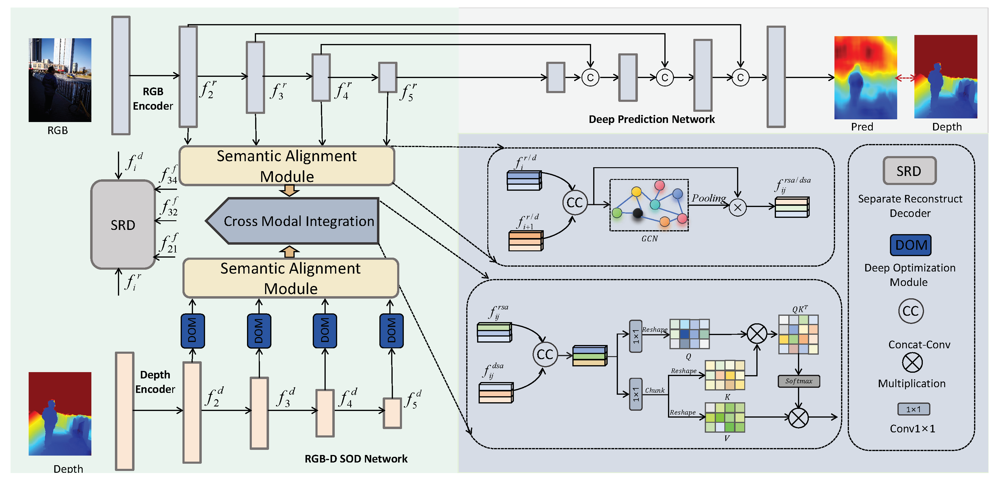
3.1. Architecture Overview

Figure 2 illustrates the overview architecture of our proposed MLBSNet model. Based on an end-to-end architecture, it contains two branch networks: depth prediction and RGB-D SOD network. In RGB-D SOD, the main components include depth optimization, a semantic alignment module, cross-modal integration, and a separate–reconstruct decoder. Specifically, two parallel ResNet50 are used to extract multilevel features $f_i^r$ and $f_i^d$ from RGB and depth data, where i represents the number of layers of the encoder. After that, a U-shaped decoder is employed to complete the depth prediction and output the feature $M_p$. To obtain more accurate depth maps, we propose a depth optimization module (DOM) to balance the error caused by unstable depth maps. A semantic alignment module (SAM) is designed to strengthen the links between neighboring feature layers and reduce fusion variability. Next, a cross-modal integration module is implemented to enable the fusion of RGB and depth features. Finally, a separation–reconstruction decoder is designed to segment out saliency objects.

Figure 2. The overall architecture of the proposed MLBSNet.

3.2. Depth Optimization Module (DOM)

As mentioned above, unstable depth maps may provide inaccurate depth information, which may pose challenges for cross-modal fusion. To solve this problem, as shown in Figure 3, we propose a depth optimization module that learns more effective depth information between the predicted depth and the original depth. Specifically, we first predict pseudo-depth maps from RGB images utilizing a depth prediction network. In addition, the predicted depth features that are used to perform the optimization maintain the D-dimensional. Empirically, D is set to 128, which maintains a wealth of depth information. With multilayer perceptron (MLP) operations, we input the output feature into the cosine function to compute the similarity between $M_o$ and $M_f$, and between $M_f$ and $M_p$, respectively. The above process is expressed as follows:

$$\begin{array}{cc}\hfill & M_f=CC(M_o,M_p),\hfill \\ \hfill & S_1=cos\left(MLP(M_o,M_f)\right),\hfill \\ \hfill & S_2=cos\left(MLP(M_f,M_p)\right),\hfill \end{array}$$

(1)

where $CC$ denotes concatenation and convolutions, $M_p$ denotes the predicted depth features, $MLP$ denotes the multilayer perceptron, $cos$ denotes the cosine function, and $S_1$ and $S_2$ denote the similarity values of $M_o$, $M_f$, and $M_f$, $M_p$ respectively.

Figure 3. Architecture of the proposed DOM.

3.3. Semantic Alignment Module (SAM)

Considering the matching problem between the neighboring hierarchical features of a single modality, SAM is proposed to balance the variability between the neighboring features in terms of details and enhance its semantic relevance. Inspired by [36], graph convolutional network operations can be used to explore semantic correlations between different pixels to learn more discriminative information. Next, concatenation and convolution are employed to extract features $f_i^{r/d}$ and $f_{i+1}^{r/d}$$(i\in 2,3,4)$, followed by a graph convolutional network and a pooling operation to learn more subtle features. The above process is expressed as follows:

$$\begin{array}{cc}\hfill & f_{ij}^{rsa/dsa}=CC(f_i^{d/r},f_{i+1}^{d/r})\otimes Pooling\left(GCN\left(CC(f_i^{d/r},f_{i+1}^{d/r})\right)\right),\hfill \end{array}$$

(2)

where $CC$ denotes concatenate and convolution, ⊗ denotes the multiplication operation, $GCN$ denotes the graph convolutional network, $Pooling$ denotes the adaptive averaging pooling operation, and $f_{ij}^{rsa/dsa}$ denotes the output features of SAM, where $j=i+1$.

3.4. Cross-Modal Integration (CMI) Module

To extract cross-modal features, a cross-modal integration module is proposed to learn more common representations between RGB images and depth maps. As shown in Figure 2, we integrate the feature output from SAM through concatenation and convolution operations. We use two $1\times 1$ convolutions separately for the feature extraction of the features being integrated. After the reshaping and chunking operations, we obtain the features Q, K, and V. After that, we obtain the weight map $Q{K}^T$ by matrix multiplication and softmax operation. The last multiplication operation is used to enhance the feature V. The above process is represented as follows:

$$\begin{array}{cc}\hfill & Q=Reshape\left(con{v}_{1\times 1}\left(CC(f_{ij}^{rsa},f_{ij}^{dsa})\right)\right),\hfill \\ \hfill & K=Reshape\left(Chunk\left(con{v}_{1\times 1}\left(CC(f_{ij}^{rsa},f_{ij}^{dsa})\right)\right)\right),\hfill \\ \hfill & V=Reshape\left(Chunk\left(con{v}_{1\times 1}\left(CC(f_{ij}^{rsa},f_{ij}^{dsa})\right)\right)\right),\hfill \\ \hfill & f_{ij}^f=softmax(Q\otimes K^T)\otimes V\hfill \end{array}$$

(3)

where $CC$ denotes concatenate and convolution, ⊗ denotes the multiplication operation, and $Chunk$ denotes the channel split operation.

3.5. Separate–Reconstruct Decoder (SRD)

We propose the SRD module in response to the question of how to make the best use of multiple sources of information. As shown in Figure 4, the module first integrates the fused features from all the outputs in the encoder. Considering the interdependence of features between channels, we performed a channel shuffling operation before separating the features, which allowed the network to learn different features, thus increasing the robustness of the model. Afterward, the separated features are combined with RGB and depth maps from different levels in the encoder to learn the saliency information provided in different modalities. To fully utilize features from different sources, we also propose a multi-source feature (MSF) integration module to learn more discriminative features to highlight saliency objects. The output features are then multiplied with RGB and depth maps to obtain enhanced features. It is worth noting that we use top-down reconstruction to gradually refine the segmentation target, which preserves more delicate saliency target details. The above process is represented as follows:

$$\begin{array}{cc}\hfill & X_1,X_2,\dots ,X_n=split\left(shuffle\left(CC(f_{45}^f,f_{34}^f,f_{23}^f)\right)\right),\hfill \\ \hfill & F_i^f=f_i^r\otimes CC(X_i,F_{i-1}^f)+f_i^d\otimes CC(X_i,F_{i-1}^f),\hfill \end{array}$$

(4)

where $CC$ denotes concatenate and convolution, ⊗ denotes the multiplication operation, $split$ indicates the channel split operation, and $shuffle$ denotes the channel shuffle operation.

Figure 4. Architecture of the proposed SRD.

3.6. Supervision

Our network is an end-to-end training process. The overall loss function is described as follows:

$${\mathcal{L}}_{total}={\mathcal{L}}_D+{\mathcal{L}}_S+{\mathcal{L}}_O,$$

(5)

We follow previous work [37] in the depth prediction phase, using SSIM and L1 as loss functions to predict the depth map. Following [38], we introduce a difference minimization loss ${\mathcal{L}}_M$ to reduce the difference between the predicted depth map and the depth map.

$$\begin{array}{cc}\hfill & {\mathcal{L}}_D={\mathcal{L}}_{SSIM}(M_o,M_p)+{\mathcal{L}}_{L1}+{\mathcal{L}}_M(M_o,M_p),\hfill \\ \hfill & {\mathcal{L}}_M={\mathcal{L}}_{ce}(M_p,M_o)+{\mathcal{L}}_{ce}((M_o,M_p)+KL(M_p,M_o)+KL(M_o,M_p),\hfill \end{array}$$

(6)

where ${\mathcal{L}}_{ce}$ denotes the binary cross-entropy loss, $KL$ denotes Kullback–Leibler divergence, $M_p$ denotes the predicted depth map, and $M_o$ denotes the original depth map. This $KL$ loss is used to measure the similarity between the two modalities.

In the depth optimization phase, we use the cosine function as a similarity loss to predict more useful depth features. In the saliency prediction stage, we use the commonly used binary cross-entropy loss and IoU loss to optimize the network.

$${\mathcal{L}}_O=cos(M_c,M_p)+cos(M_c,M_o),$$

(7)

$${\mathcal{L}}_S=\sum _{i=1}^4({\mathcal{L}}_{bce}(S,G)+{\mathcal{L}}_{iou}(S,G)),$$

(8)

where S denotes the saliency map, G denotes the ground truth map, and $M_c$ denotes the optimized depth map.

4. Experiments

4.1. Experimental Protocol

Datasets. For a fair comparison, we followed previous works [11,39] and selected 1485 images from the NJU2K [40] dataset and 700 images from the NLPR [41] dataset for training. We then tested the performance of our model and existing RGB-D saliency detection models on the NJU2K, NLPR, LFSD [42], DES [21], SIP [13], and STERE [43] test sets.

Evaluation metrics. We used four widely used metrics in our quantitative comparisons: mean absolute error ($MAE$) [44], S-measure ($S_m$) [45], maximum F-measure ($F_{\beta }$) [46], and maximum E-measure ($E_m$) [47]. $MAE$ was used to express the pixel-by-pixel mean absolute error between the predicted saliency map and the ground truth. S-measure is used to measure the structural integrity of the predictions. F-measure is used to balance precision and recall. E-measure is used to obtain image-level statistics and local pixel information.

Implementation details. Our model was implemented based on Pytorch and trained 120 times on an A4000 GPU, taking 6 h. We chose ResNet50 [48] as the backbone network for our model, and the network parameters were initialized by a pre-trained model on ImageNet [49]. The input RGB and depth map sizes were resized to 352 × 352 during both the training and testing phases. In addition, we utilized the Adam algorithm to optimize the network. The learning rate was set to 0.0001, and the batch size was set to 10. To avoid overfitting, we augmented the data with random flipping, rotating, and clipping.

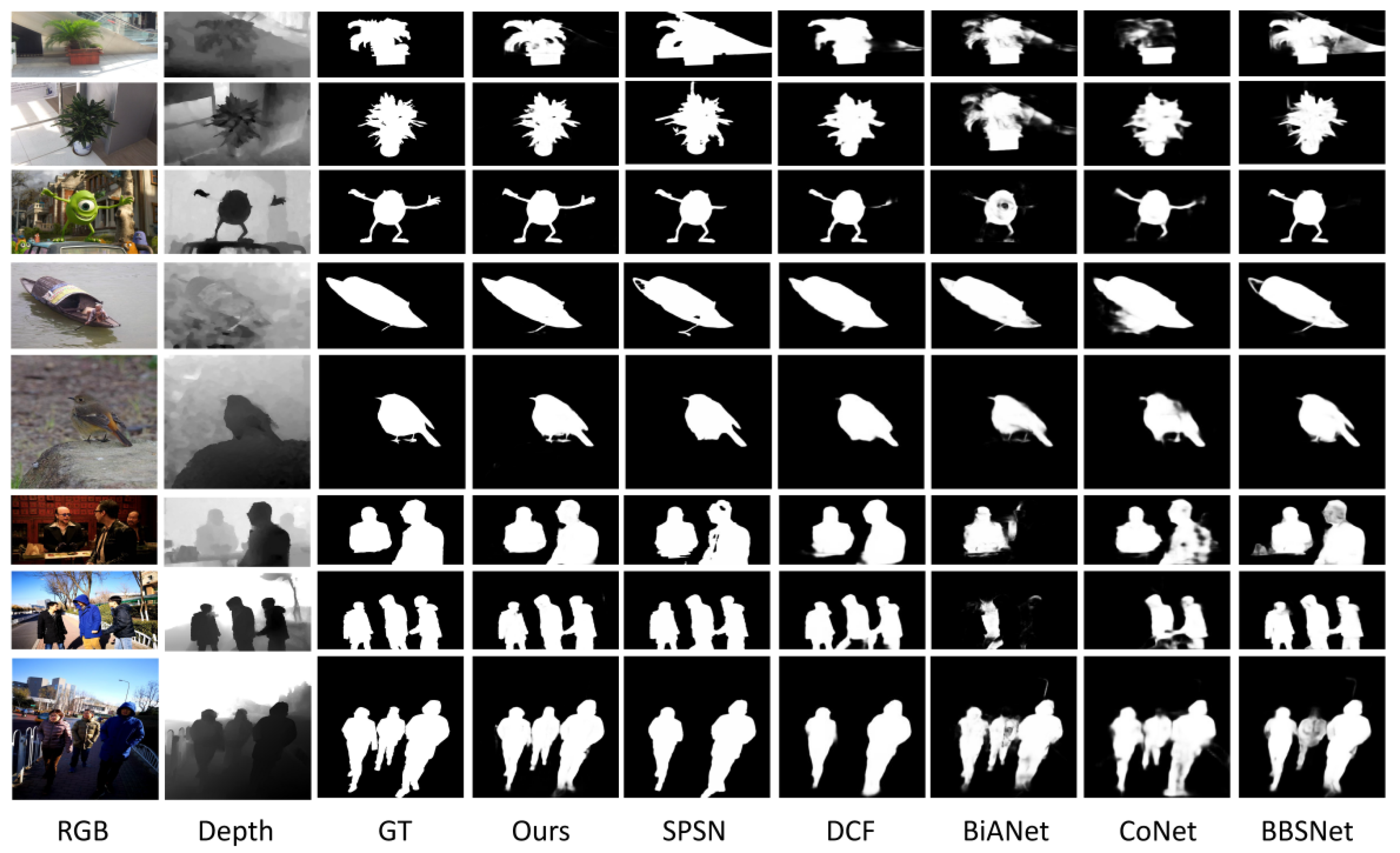
4.2. Comparison with State-of-the-Art Models

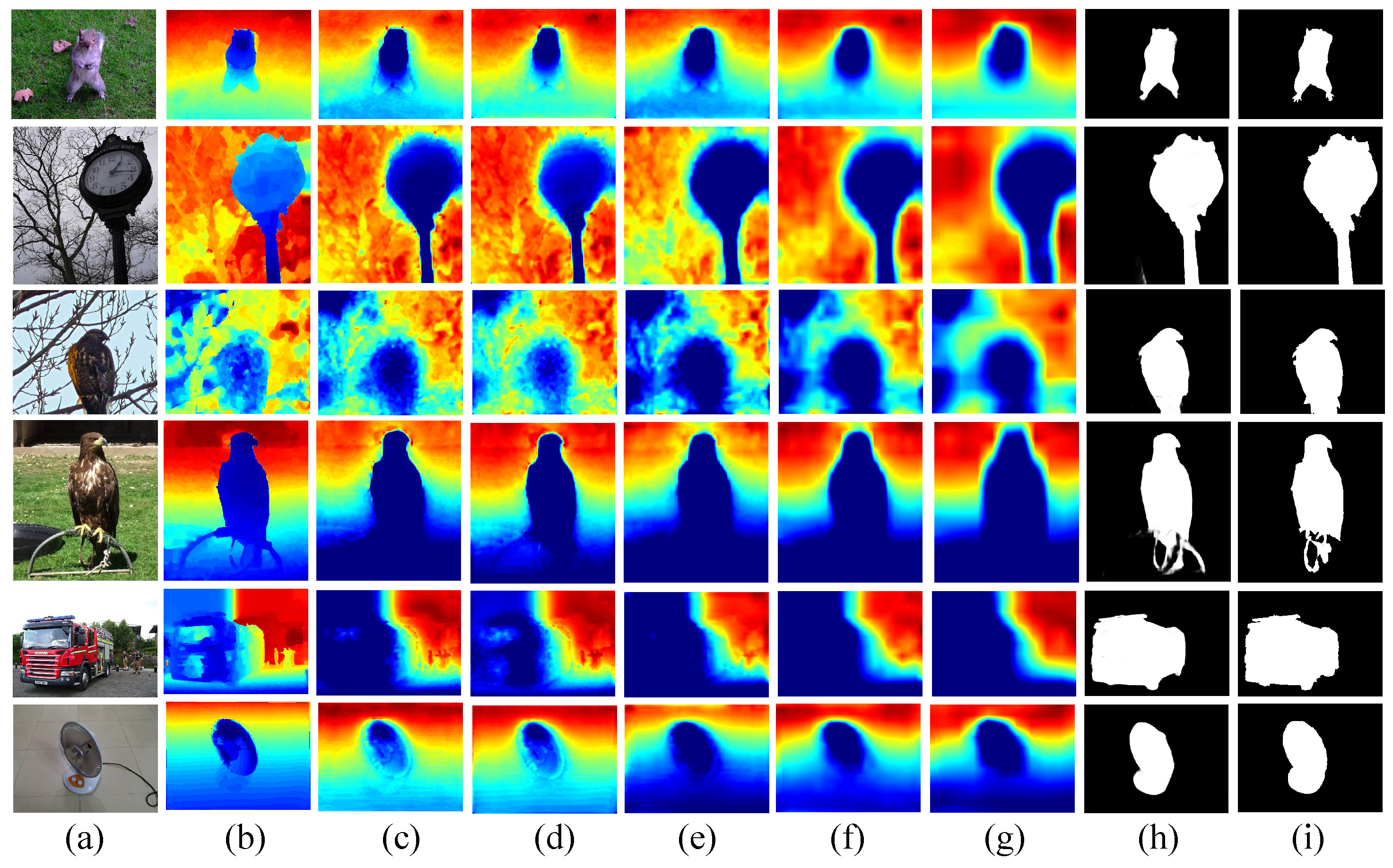
We compare with 13 state-of-the-art models, including DGFNet [50], MRVI [51], SPSN [6], EMANet [30], SMAC [52], AirSOD [53], HINet [54], DCF [11], BBSNet [39], BiANet [55], JLDCF [56], D3Net [13], and CoNet [57]. In this study, we test the performance results using the authors’ prediction maps and the code generation result maps.

As shown in Figure 5, it can be observed through the PR curves that MLBSNet achieves significantly improved performance on the five datasets. Table 1 shows the quantitative comparison results of our model on the five datasets. Our model achieves excellent performance on all four evaluation metrics. In particular, the model outperforms all state-of-the-art models on the NJU2K and STERE datasets. This reflects the good generalization ability of the model. Regarding $MAE$ metrics, our method achieves a minimum percentage gain of $5.8\%$ for DES, $4.6\%$ for SIP, $10.2\%$ for STERE, and $9.3\%$ for NJU2K compared to the second-best method. In terms of $F_{\beta }$ metrics, our method reaches a minimum percentage gain of $0.8\%$ in NJU2K and $0.7\%$. Figure 6 visualizes the results of the qualitative comparison between MLBSNet and other state-of-the-art methods. Our method achieves better detection results in some complex scenes. For example, in the first and second rows, for detecting plants with complex edges, our proposed method can segment the edges of the plants more accurately compared to other methods. In the third row, the salient object in the RGB image is in a situation where the background is cluttered and the depth information is missing, but our proposed method still segments the salient object completely. Some incorrect depth maps may provide noise for fusion, and in the fourth row, our proposed method obtains accurate results. Benefiting from the proposed CMI module makes the network more robust. In the fifth row, our proposed method still extracts the salient objects completely in the face of the foreground–background similarity in RGB images and the continuous distribution of depth values of salient and non-salient objects in the depth map. These results are more dependent on the proposed DOM module, which can effectively optimize the imperfect depth map and provide effective fusion information for fusion. In the sixth, seventh, and eighth rows, our proposed method can detect multiple salient objects completely without losing the salient object information during the detection of multiple objects, while other methods failed to detect the salient information during the detection process.

Figure 5. The PR curves on NJU2K [58], NLPR [41], SIP [13], DES [21], and STERE [43].

Table 1. The quantitative comparison of our proposed model with 13 state-of-the-art RGB-D saliency models on five benchmark datasets. Red color indicates the best result, and blue color indicates the second-best result. The ↑/↓ means that the larger/smaller value is better.

Dataset	Metric	D3Net20	BBSNet20	CoNet20	JLDCF21	DCF21	BiANet21	EMANet22	SPSN22	SMAC22	AirSOD22	HINet23	MRVI23	DGFNet23	Ours
NJU2K	$E_m\uparrow$	0.950	$0.942$	$0.936$	$0.926$	$0.946$	$0.941$	$0.946$	$0.949$	$0.937$	$0.944$	$0.945$	$0.929$	-	0.953
	$S_m\uparrow$	$0.900$	0.920	$0.896$	$0.902$	$0.912$	$0.917$	$0.923$	$0.918$	$0.903$	$0.908$	$0.914$	$0.890$	0.920	0.925
	$F_{\beta }\uparrow$	$0.900$	0.931	$0.902$	$0.912$	$0.922$	$0.929$	$0.914$	$0.927$	$0.896$	$0.918$	$0.915$	$0.880$	$0.912$	0.939
	$MAE\downarrow$	$0.041$	$0.035$	$0.046$	$0.041$	$0.036$	$0.036$	$0.035$	0.032	$0.044$	$0.039$	$0.039$	$0.046$	$0.033$	0.029
NLPR	$E_m\uparrow$	$0.953$	$0.956$	$0.955$	$0.955$	0.958	$0.953$	$0.955$	$0.956$	$0.953$	$0.924$	0.957	$0.953$	-	$0.956$
	$S_m\uparrow$	$0.912$	$0.926$	$0.925$	$0.925$	$0.924$	0.930	$0.922$	$0.923$	$0.922$	$0.924$	$0.906$	$0.914$	$0.923$	0.926
	$F_{\beta }\uparrow$	$0.897$	$0.924$	0.925	$0.925$	$0.918$	0.927	$0.924$	$0.917$	$0.904$	$0.923$	$0.922$	$0.895$	$0.893$	$0.924$
	$MAE\downarrow$	$0.030$	$0.023$	$0.022$	$0.022$	$0.022$	$0.023$	$0.024$	0.023	$0.027$	$0.023$	$0.026$	$0.025$	$0.025$	0.022
DES	$E_m\uparrow$	$0.946$	$0.958$	$0.961$	$0.961$	$0.944$	$0.955$	$0.953$	0.973	$0.972$	$0.962$	-	$0.965$	-	0.974
	$S_m\uparrow$	$0.898$	$0.930$	$0.931$	$0.931$	$0.905$	$0.934$	$0.930$	0.937	$0.935$	$0.923$	-	$0.928$	$0.931$	0.940
	$F_{\beta }\uparrow$	$0.885$	$0.930$	$0.934$	$0.934$	$0.910$	0.942	$0.915$	0.942	$0.926$	$0.934$	-	$0.921$	$0.916$	0.943
	$MAE\downarrow$	$0.031$	$0.020$	$0.020$	$0.020$	$0.024$	$0.021$	$0.023$	0.017	$0.020$	$0.022$	-	$0.019$	$0.018$	0.016
SIP	$E_m\uparrow$	$0.909$	$0.920$	$0.918$	$0.918$	$0.916$	$0.910$	-	-	0.932	$0.925$	$0.903$	-	$0.924$	0.930
	$S_m\uparrow$	$0.860$	$0.887$	$0.880$	$0.880$	$0.876$	$0.879$	-	0.891	$0.883$	$0.858$	-	$0.876$	-	0.895
	$F_{\beta }\uparrow$	$0.861$	$0.904$	0.903	0.903	$0.899$	$0.902$	-	0.910	$0.886$	$0.887$	-	$0.863$	-	0.910
	$MAE\downarrow$	$0.063$	$0.047$	$0.049$	$0.049$	$0.052$	$0.055$	-	0.043	$0.049$	$0.060$	-	$0.049$	-	0.041
STERE	$E_m\uparrow$	$0.938$	$0.935$	$0.934$	$0.934$	$0.940$	$0.931$	$0.939$	$0.941$	0.941	$0.939$	$0.933$	-	-	0.942
	$S_m\uparrow$	$0.899$	$0.905$	$0.903$	$0.903$	$0.902$	$0.908$	0.911	$0.906$	$0.905$	$0.895$	$0.883$	-	$0.906$	0.912
	$F_{\beta }\uparrow$	$0.891$	$0.912$	$0.913$	$0.913$	$0.911$	0.919	$0.901$	$0.909$	$0.897$	$0.900$	$0.892$	-	$0.906$	0.920
	$MAE\downarrow$	$0.046$	0.039	$0.040$	$0.040$	0.039	$0.041$	$0.040$	0.035	$0.042$	$0.043$	$0.049$	-	$0.038$	0.035

Figure 6. Visual comparison of different methods.

4.3. Ablation Study

To verify the usefulness of the different modules in our proposed model, we demonstrate the validity of the added modules by removing them from the complete model.

Effectiveness of the depth optimization module. To demonstrate the effectiveness of the added depth optimization module, we removed the module from the network and labeled it as w/o DOM. As seen in Table 2, compared to w/o DOM, our proposed method resulted in a percentage gain of $3.4\%$ on the $MAE$ of NJU2K and a percentage gain of $12.7\%$ on the $MAE$ of SIP. In addition, our method increases the value of $F_{\beta }$ from 0.904 to 0.910 on the SIP dataset. Our proposed depth optimization module can largely improve the quality of the depth map to enhance the performance of the model. As seen from column (e) in Figure 7, removing the DOM module makes the network produce a lot of interfering information. In addition, to demonstrate the effect of the proposed module on the depth map, we visualized the depth map at different stages, as shown in Figure 8. To further illustrate the impact of the proposed supervised learning on the model performance, we remove ${\mathcal{L}}_O$. As can be seen in Table 2, all metrics are greatly improved on the DES, NJU2K, and SIP datasets. Therefore, similarity learning can learn deep information more reliably. To demonstrate the effectiveness of the proposed ${\mathcal{L}}_M$ even further, we delete ${\mathcal{L}}_M$ and only keep ${\mathcal{L}}_O$. As shown in Table 3, the model’s performance is greatly improved.

Table 2. Quantitative comparison of ablation experiments on NJU2K and SIP datasets, with ↑/↓ denoting that the larger/smaller value is better.

Virants	NJU2K				SIP
	${\mathit{F}}_{\mathit{\beta }}\uparrow$	${\mathit{S}}_{\mathit{m}}\uparrow$	${\mathit{E}}_{\mathit{m}}\uparrow$	$\mathit{MAE}\downarrow$	${\mathit{F}}_{\mathit{\beta }}\uparrow$	${\mathit{S}}_{\mathit{m}}\uparrow$	${\mathit{E}}_{\mathit{m}}\uparrow$	$\mathit{MAE}\downarrow$
w/o DOM	0.935	0.923	0.951	0.030	0.904	0.885	0.920	0.047
w/o SAM	0.936	0.923	0.951	0.031	0.908	0.889	0.924	0.045
w/o CIM	0.937	0.922	0.950	0.031	0.907	0.889	0.923	0.045
w/o SRD	0.926	0.914	0.944	0.034	0.907	0.891	0.930	0.044
Ours	0.939	0.925	0.953	0.029	0.910	0.895	0.930	0.041

Figure 7. Comparison of ablation experiment visualizations: (a) RGB; (b) depth; (c) GT; (d) saliency maps obtained by MLBSNet; (e) saliency maps obtained by w/o DOM; (f) saliency maps obtained by w/o SAM; (g) saliency maps obtained by w/o CIM; (h) saliency maps obtained by w/o SAM.

Figure 8. Visualisation of depth maps at different stages:(a) RGB; (b) depth; (c) predicted depth maps; (d) the depth maps obtained by the DOM module in layer 2; (e) the depth maps obtained by the DOM module in layer 3; (f) the depth maps obtained by the DOM module in layer 4; (g) the depth maps obtained by the DOM module in layer 5; (h) saliency maps obtained by MLBSNet; (i) GT.

Table 3. Ablation experiments on supervise learning, with ↑/↓ denoting that the larger/smaller value is better.

${\mathcal{L}}_{\mathit{O}}$	${\mathcal{L}}_{\mathit{M}}$	SIP			DES			NJU2K
		${\mathit{S}}_{\mathit{m}}\uparrow$	${\mathit{F}}_{\mathit{\beta }}\uparrow$	${\mathit{E}}_{\mathit{m}}\uparrow$	${\mathit{S}}_{\mathit{m}}\uparrow$	${\mathit{F}}_{\mathit{\beta }}\uparrow$	${\mathit{E}}_{\mathit{m}}\uparrow$	${\mathit{S}}_{\mathit{m}}\uparrow$	${\mathit{F}}_{\mathit{\beta }}\uparrow$	${\mathit{E}}_{\mathit{m}}\uparrow$
✓		0.888	0.906	0.922	0.938	0.941	0.971	0.920	0.933	0.949
	✓	0.886	0.904	0.922	0.933	0.938	0.968	0.922	0.936	0.950
✓	✓	0.895	0.910	0.930	0.940	0.943	0.974	0.925	0.939	0.953

Effectiveness of the semantic alignment module. To prove the effectiveness of the added semantic alignment module, we delete the module in the network and only carry out the channel splicing operation on the neighboring features and mark it as w/o SAM. As shown in Table 2, the added semantic alignment module can better learn the features of the neighboring levels and reduce the differences between the different levels of modalities, thus enhancing the relevance of the neighboring features and improving the model’s performance. Our proposed method has a gain of $6.4\%$ on the $MAE$ of NJU2K and $8.8\%$ on the $MAE$ of SIP. In addition, our method increases $S_m$ from a value of 0.889 to 0.895 on the SIP dataset, and $E_m$ from 0.924 to 0.930. The semantic alignment module can obtain more significant information for subsequent fusion, which in turn improves the model performance.

Effectiveness of the cross-modal integration module. To demonstrate the importance of the added cross-modal integration module, we removed the module from the network and only performed simple addition operations on the RGB and depth maps and labeled it as w/o CIM. Table 2 shows that the added cross-modal integration module facilitates performance improvement. On both the NJU2K and SIP datasets, all four metrics were greatly improved. Especially on the $S_m$ metric, $S_m$ increases from 0.922 to 0.925 on the NJU2K dataset, and $S_m$ improves from 0.923 to 0.930 on the SIP dataset. These results demonstrate that the cross-modal integration module can efficiently fuse the RGB image and depth information and promote the expression of saliency objects.

Effectiveness of separate–reconstruct decoder. To demonstrate the contribution of the designed decoder to the model’s performance, we used a U-shaped network for the substitution and labeled it as w/o SRD. As demonstrated in Table 2 and Figure 7, the separate–reconstruct decoder helps to improve the model performance and maintain the details of the saliency objects. The percentage gain on $MAE$ is $16.1\%$ and $7.3\%$ respectively. $S_m$ metrics on NJU2K is $1.1\%$. The $F_{\beta }$ metric has a percentage gain of $1.3\%$ on NJU2K. These results show that our proposed decoder can learn saliency features and separate saliency objects from multi-source information compared to the U-decoder.

Efficiency evaluation. To demonstrate the efficiency of the proposed model even further, we compare the inference time (fps), model complexity (FLOPs), and number of parameters of the proposed model with other models. For a fair comparison, all models are computed on 3090 GPUs. As shown in Table 4, our model has relatively lower FLOPs and faster fps compared to other approaches.

Table 4. Parameters, FLOPs, and fps of different RGB-D SOD methods.

Models	Backbone	Input Size	FLOPs (G)	Parameters (M)	fps
BBSNet [39]	ResNet50	352 × 352	62.6	49.7	25
BiANet [55]	ResNet50	352 × 352	115.1	63.7	30
CIRNet [32]	ResNet50	352 × 352	85.2	103.1	26
SPSN [6]	VGG16	352 × 352	501.6	37	-
Ours	ResNet50	352×352	75.2	106.2	41

5. Conclusions

We propose a mutual learning and boosting segmentation network that completes the depth optimization, feature fusion, and information inference processes through the depth prediction and saliency object inference stages. Satisfactory results are achieved on five RGB-D saliency object detection datasets, and they outperform state-of-the-art models. First, we introduced a depth optimization module to obtain more accurate depth information through mutual learning. Then, a semantic alignment module is designed to align modalities between neighboring features. Then, the output features are fed into a cross-modal integration module to obtain complementary cross-modal information. Finally, we design a simple and effective separation–reconstruction decoder for segmenting saliency objects. In addition, predicted depth maps are not always accurate, and inaccurate depth maps may lead to optimization failures. Depth prediction networks can be added to RGB-D SOD in future works to improve the quality of depth maps and improve performance.

References

1. Yang, G.; Li, M.; Zhang, J.; Lin, X.; Ji, H.; Chang, S.F. Video event extraction via tracking visual states of arguments. In Proceedings of the AAAI Conference on Artificial Intelligence, Washington, DC, USA, 7–14 February 2023; Volume 37, pp. 3136–3144. [Google Scholar]
2. Athar, A.; Hermans, A.; Luiten, J.; Ramanan, D.; Leibe, B. Tarvis: A unified approach for target-based video segmentation. In Proceedings of the IEEE/CVF Conference on Computer Vision and Pattern Recognition, Vancouver, BC, Canada, 17–24 June 2023; pp. 18738–18748. [Google Scholar]
3. Bai, Y.; Chen, D.; Li, Q.; Shen, W.; Wang, Y. Bidirectional Copy-Paste for Semi-Supervised Medical Image Segmentation. In Proceedings of the IEEE/CVF Conference on Computer Vision and Pattern Recognition, Vancouver, BC, Canada, 17–24 June 2023; pp. 11514–11524. [Google Scholar]
4. Chai, J.C.L.; Ng, T.S.; Low, C.Y.; Park, J.; Teoh, A.B.J. Recognizability Embedding Enhancement for Very Low-Resolution Face Recognition and Quality Estimation. In Proceedings of the IEEE/CVF Conference on Computer Vision and Pattern Recognition, Vancouver, BC, Canada, 17–24 June 2023; pp. 9957–9967. [Google Scholar]
5. Chen, C.; Ye, M.; Jiang, D. Towards Modality-Agnostic Person Re-Identification with Descriptive Query. In Proceedings of the IEEE/CVF Conference on Computer Vision and Pattern Recognition, Vancouver, BC, Canada, 17–24 June 2023; pp. 15128–15137. [Google Scholar]
6. Lee, M.; Park, C.; Cho, S.; Lee, S. Spsn: Superpixel prototype sampling network for rgb-d salient object detection. In Proceedings of the European Conference on Computer Vision, Tel Aviv, Israel, 23–27 October 2022; pp. 630–647. [Google Scholar]
7. Zhou, J.; Wang, L.; Lu, H.; Huang, K.; Shi, X.; Liu, B. Mvsalnet: Multi-view augmentation for rgb-d salient object detection. In Proceedings of the European Conference on Computer Vision, Tel Aviv, Israel, 23–27 October 2022; pp. 270–287. [Google Scholar]
8. Wu, Z.; Allibert, G.; Meriaudeau, F.; Ma, C.; Demonceaux, C. HiDAnet: RGB-D Salient Object Detection via Hierarchical Depth Awareness. arXiv 2023, arXiv:2301.07405. [Google Scholar] [CrossRef] [PubMed]
9. Wu, Z.; Wang, J.; Zhou, Z.; An, Z.; Jiang, Q.; Demonceaux, C.; Sun, G.; Timofte, R. Object Segmentation by Mining Cross-Modal Semantics. arXiv 2023, arXiv:2305.10469. [Google Scholar]
10. Zhang, W.; Ji, G.P.; Wang, Z.; Fu, K.; Zhao, Q. Depth quality-inspired feature manipulation for efficient RGB-D salient object detection. In Proceedings of the 29th ACM International Conference on Multimedia, Virtual Event, 20–24 October 2021; pp. 731–740. [Google Scholar]
11. Ji, W.; Li, J.; Yu, S.; Zhang, M.; Piao, Y.; Yao, S.; Bi, Q.; Ma, K.; Zheng, Y.; Lu, H.; et al. Calibrated RGB-D salient object detection. In Proceedings of the IEEE Conference on Computer Vision and Pattern Recognition, Nashville, TN, USA, 20–25 June 2021; pp. 9471–9481. [Google Scholar]
12. Zhang, Q.; Qin, Q.; Yang, Y.; Jiao, Q.; Han, J. Feature Calibrating and Fusing Network for RGB-D Salient Object Detection. IEEE Trans. Circuits Syst. Video Technol. 2023, 34, 1493–1507. [Google Scholar] [CrossRef]
13. Fan, D.P.; Lin, Z.; Zhang, Z.; Zhu, M.; Cheng, M.M. Rethinking RGB-D salient object detection: Models, data sets, and large-scale benchmarks. IEEE Trans. Neural Netw. Learn. Syst. 2020, 32, 2075–2089. [Google Scholar] [CrossRef] [PubMed]
14. Chen, C.; Wei, J.; Peng, C.; Zhang, W.; Qin, H. Improved saliency detection in RGB-D images using two-phase depth estimation and selective deep fusion. IEEE Trans. Image Process. 2020, 29, 4296–4307. [Google Scholar] [CrossRef]
15. Zhao, J.; Zhao, Y.; Li, J.; Chen, X. Is depth really necessary for salient object detection? In Proceedings of the 28th ACM International Conference on Multimedia, Seattle, WA, USA, 12–16 October 2020; pp. 1745–1754. [Google Scholar]
16. Wu, Z.; Gobichettipalayam, S.; Tamadazte, B.; Allibert, G.; Paudel, D.P.; Demonceaux, C. Robust rgb-d fusion for saliency detection. In Proceedings of the 2022 International Conference on 3D Vision (3DV), Prague, Czechia, 12–15 September 2022; pp. 403–413. [Google Scholar]
17. Song, M.; Song, W.; Yang, G.; Chen, C. Improving RGB-D salient object detection via modality-aware decoder. IEEE Trans. Image Process. 2022, 31, 6124–6138. [Google Scholar] [CrossRef] [PubMed]
18. Sun, F.; Ren, P.; Yin, B.; Wang, F.; Li, H. CATNet: A Cascaded and Aggregated Transformer Network For RGB-D Salient Object Detection. IEEE Trans. Multimed. 2023, 26, 2249–2262. [Google Scholar] [CrossRef]
19. Wen, H.; Yan, C.; Zhou, X.; Cong, R.; Sun, Y.; Zheng, B.; Zhang, J.; Bao, Y.; Ding, G. Dynamic selective network for RGB-D salient object detection. IEEE Trans. Image Process. 2021, 30, 9179–9192. [Google Scholar] [CrossRef]
20. Ji, W.; Yan, G.; Li, J.; Piao, Y.; Yao, S.; Zhang, M.; Cheng, L.; Lu, H. DMRA: Depth-induced multi-scale recurrent attention network for RGB-D saliency detection. IEEE Trans. Image Process. 2022, 31, 2321–2336. [Google Scholar] [CrossRef]
21. Cheng, Y.; Fu, H.; Wei, X.; Xiao, J.; Cao, X. Depth enhanced saliency detection method. In Proceedings of the International Conference on Internet Multimedia Computing and Service, Xiamen, China, 10–12 July 2014; pp. 23–27. [Google Scholar]
22. Ciptadi, A.; Hermans, T.; Rehg, J.M. An In Depth View of Saliency. In Proceedings of the BMVC, Bristol, UK, 9–13 September 2013; pp. 1–11. [Google Scholar]
23. Piao, Y.; Rong, Z.; Zhang, M.; Ren, W.; Lu, H. A2dele: Adaptive and attentive depth distiller for efficient RGB-D salient object detection. In Proceedings of the IEEE/CVF Conference on Computer Vision and Pattern Recognition, Seattle, WA, USA, 13–19 June 2020; pp. 9060–9069. [Google Scholar]
24. Zhang, C.; Cong, R.; Lin, Q.; Ma, L.; Li, F.; Zhao, Y.; Kwong, S. Cross-modality discrepant interaction network for RGB-D salient object detection. In Proceedings of the ACM International Conference on Multimedia, Virtual Event, 20–24 October 2021; pp. 2094–2102. [Google Scholar]
25. Liao, G.; Gao, W.; Jiang, Q.; Wang, R.; Li, G. Mmnet: Multi-stage and multi-scale fusion network for rgb-d salient object detection. In Proceedings of the 28th ACM International Conference on Multimedia, Seattle, WA, USA, 12–16 October 2020; pp. 2436–2444. [Google Scholar]
26. Qu, L.; He, S.; Zhang, J.; Tian, J.; Tang, Y.; Yang, Q. RGBD salient object detection via deep fusion. IEEE Trans. Image Process. 2017, 26, 2274–2285. [Google Scholar] [CrossRef]
27. Zhang, J.; Fan, D.P.; Dai, Y.; Anwar, S.; Saleh, F.S.; Zhang, T.; Barnes, N. UC-Net: Uncertainty inspired RGB-D saliency detection via conditional variational autoencoders. In Proceedings of the IEEE Conference on Computer Vision and Pattern Recognition, Seattle, WA, USA, 13–19 June 2020; pp. 8582–8591. [Google Scholar]
28. Han, J.; Chen, H.; Liu, N.; Yan, C.; Li, X. CNNs-based RGB-D saliency detection via cross-view transfer and multiview fusion. IEEE Trans. Cybern. 2017, 48, 3171–3183. [Google Scholar] [CrossRef] [PubMed]
29. Wang, Y.; Wang, F.; Wang, C.; Sun, F.; He, J. Learning Saliency-Aware Correlation Filters for Visual Tracking. Comput. J. 2022, 65, 1846–1859. [Google Scholar] [CrossRef]
30. Feng, G.; Meng, J.; Zhang, L.; Lu, H. Encoder deep interleaved network with multi-scale aggregation for RGB-D salient object detection. Pattern Recognit. 2022, 128, 108666. [Google Scholar] [CrossRef]
31. Sun, P.; Zhang, W.; Wang, H.; Li, S.; Li, X. Deep RGB-D saliency detection with depth-sensitive attention and automatic multi-modal fusion. In Proceedings of the IEEE Conference on Computer Vision and Pattern Recognition, Nashville, TN, USA, 20–25 June 2021; pp. 1407–1417. [Google Scholar]
32. Cong, R.; Lin, Q.; Zhang, C.; Li, C.; Cao, X.; Huang, Q.; Zhao, Y. CIR-Net: Cross-modality interaction and refinement for RGB-D salient object detection. IEEE Trans. Image Process. 2022, 31, 6800–6815. [Google Scholar] [CrossRef] [PubMed]
33. Zhou, T.; Fu, H.; Chen, G.; Zhou, Y.; Fan, D.P.; Shao, L. Specificity-preserving RGB-D saliency detection. In Proceedings of the IEEE/CVF International Conference on Computer Vision, Montreal, QC, Canada, 10–17 October 2021; pp. 4681–4691. [Google Scholar]
34. Zhou, W.; Zhu, Y.; Lei, J.; Wan, J.; Yu, L. CCAFNet: Crossflow and cross-scale adaptive fusion network for detecting salient objects in RGB-D images. IEEE Trans. Multimed. 2021, 24, 2192–2204. [Google Scholar] [CrossRef]
35. Jin, W.D.; Xu, J.; Han, Q.; Zhang, Y.; Cheng, M.M. CDNet: Complementary depth network for RGB-D salient object detection. IEEE Trans. Image Process. 2021, 30, 3376–3390. [Google Scholar] [CrossRef] [PubMed]
36. Te, G.; Liu, Y.; Hu, W.; Shi, H.; Mei, T. Edge-aware graph representation learning and reasoning for face parsing. In Proceedings of the Computer Vision–ECCV 2020: 16th European Conference, Glasgow, UK, 23–28 August 2020; Proceedings, Part XII 16. Springer: Berlin/Heidelberg, Germany, 2020; pp. 258–274. [Google Scholar]
37. Zhao, X.; Pang, Y.; Zhang, L.; Lu, H. Joint learning of salient object detection, depth estimation and contour extraction. IEEE Trans. Image Process. 2022, 31, 7350–7362. [Google Scholar] [CrossRef] [PubMed]
38. Zhang, J.; Fan, D.P.; Dai, Y.; Yu, X.; Zhong, Y.; Barnes, N.; Shao, L. RGB-D saliency detection via cascaded mutual information minimization. In Proceedings of the IEEE/CVF International Conference on Computer Vision, Montreal, BC, Canada, 11–17 October 2021; pp. 4338–4347. [Google Scholar]
39. Fan, D.P.; Zhai, Y.; Borji, A.; Yang, J.; Shao, L. BBS-Net: RGB-D salient object detection with a bifurcated backbone strategy network. In Proceedings of the European Conference on Computer Vision, Glasgow, UK, 23–28 August 2020; pp. 275–292. [Google Scholar]
40. Ju, R.; Ge, L.; Geng, W.; Ren, T.; Wu, G. Depth saliency based on anisotropic center-surround difference. In Proceedings of the 2014 IEEE International Conference on Image Processing (ICIP), Paris, France, 27–30 October 2014; pp. 1115–1119. [Google Scholar]
41. Peng, H.; Li, B.; Xiong, W.; Hu, W.; Ji, R. RGBD salient object detection: A benchmark and algorithms. In Proceedings of the Computer Vision–ECCV 2014: 13th European Conference, Zurich, Switzerland, 6–12 September 2014; Proceedings, Part III 13. Springer: Berlin/Heidelberg, Germany, 2014; pp. 92–109. [Google Scholar]
42. Li, N.; Ye, J.; Ji, Y.; Ling, H.; Yu, J. Saliency detection on light field. In Proceedings of the IEEE Conference on Computer Vision and Pattern Recognition, Columbus, OH, USA, 23–28 June 2014; pp. 2806–2813. [Google Scholar]
43. Niu, Y.; Geng, Y.; Li, X.; Liu, F. Leveraging stereopsis for saliency analysis. In Proceedings of the 2012 IEEE Conference on Computer Vision and Pattern Recognition, Providence, RI, USA, 16–21 June 2012; pp. 454–461. [Google Scholar]
44. Perazzi, F.; Krahenbuhl, P.; Pritch, Y.; Hornung, A. Saliency filters: Contrast based filtering for salient region detection. In Proceedings of the IEEE Conference on Computer Vision and Pattern Recognition, Providence, RI, USA, 16–21 June 2012; pp. 733–740. [Google Scholar]
45. Fan, D.P.; Cheng, M.M.; Liu, Y.; Li, T.; Borji, A. Structure-measure: A new way to evaluate foreground maps. In Proceedings of the IEEE International Conference on Computer Vision, Venice, Italy, 22–29 October 2017; pp. 4548–4557. [Google Scholar]
46. Kulshreshtha, A.; Deshpande, A.; Meher, S.K. Time-frequency-tuned salient region detection and segmentation. In Proceedings of the IEEE International Advance Computing Conference, Ghaziabad, India, 22–23 February 2013; pp. 1080–1085. [Google Scholar]
47. Fan, D.P.; Gong, C.; Cao, Y.; Ren, B.; Cheng, M.M.; Borji, A. Enhanced-alignment measure for binary foreground map evaluation. arXiv 2018, arXiv:1805.10421. [Google Scholar]
48. He, K.; Zhang, X.; Ren, S.; Sun, J. Deep residual learning for image recognition. In Proceedings of the IEEE Conference on Computer Vision and Pattern Recognition, Las Vegas, NV, USA, 27–30 June 2016; pp. 770–778. [Google Scholar]
49. Russakovsky, O.; Deng, J.; Su, H.; Krause, J.; Satheesh, S.; Ma, S.; Huang, Z.; Karpathy, A.; Khosla, A.; Bernstein, M.; et al. Imagenet large scale visual recognition challenge. Int. J. Comput. Vis. 2015, 115, 211–252. [Google Scholar] [CrossRef]
50. Xiao, F.; Pu, Z.; Chen, J.; Gao, X. DGFNet: Depth-guided cross-modality fusion network for RGB-D salient object detection. IEEE Trans. Multimed. 2023, 26, 2648–2658. [Google Scholar] [CrossRef]
51. Li, A.; Mao, Y.; Zhang, J.; Dai, Y. Mutual information regularization for weakly-supervised RGB-D salient object detection. IEEE Trans. Circuits Syst. Video Technol. 2023, 34, 397–410. [Google Scholar] [CrossRef]
52. Liu, N.; Zhang, N.; Shao, L.; Han, J. Learning selective mutual attention and contrast for RGB-D saliency detection. IEEE Trans. Pattern Anal. Mach. Intell. 2021, 44, 9026–9042. [Google Scholar] [CrossRef]
53. Zeng, Z.; Liu, H.; Chen, F.; Tan, X. AirSOD: A Lightweight Network for RGB-D Salient Object Detection. IEEE Trans. Circuits Syst. Video Technol. 2023, 34, 1656–1669. [Google Scholar] [CrossRef]
54. Bi, H.; Zhang, J.; Wu, R.; Tong, Y.; Jin, W. Cross-modal refined adjacent-guided network for RGB-D salient object detection. Multimed. Tools Appl. 2023, 82, 37453–37478. [Google Scholar] [CrossRef]
55. Zhang, Z.; Lin, Z.; Xu, J.; Jin, W.D.; Lu, S.P.; Fan, D.P. Bilateral attention network for RGB-D salient object detection. IEEE Trans. Image Process. 2021, 30, 1949–1961. [Google Scholar] [CrossRef] [PubMed]
56. Fu, K.; Fan, D.P.; Ji, G.P.; Zhao, Q.; Shen, J.; Zhu, C. Siamese network for RGB-D salient object detection and beyond. IEEE Trans. Pattern Anal. Mach. Intell. 2021, 44, 5541–5559. [Google Scholar] [CrossRef] [PubMed]
57. Ji, W.; Li, J.; Zhang, M.; Piao, Y.; Lu, H. Accurate RGB-D salient object detection via collaborative learning. In Proceedings of the European Conference on Computer Vision, Glasgow, UK, 23–28 August 2020; pp. 52–69. [Google Scholar]
58. Ju, R.; Liu, Y.; Ren, T.; Ge, L.; Wu, G. Depth-aware salient object detection using anisotropic center-surround difference. Signal Process. Image Commun. 2015, 38, 115–126. [Google Scholar] [CrossRef]
Disclaimer/Publisher’s Note: The statements, opinions and data contained in all publications are solely those of the individual author(s) and contributor(s) and not of MDPI and/or the editor(s). MDPI and/or the editor(s) disclaim responsibility for any injury to people or property resulting from any ideas, methods, instructions or products referred to in the content.
Article Metrics
Citations
Article Access Statistics
Multiple requests from the same IP address are counted as one view.