Feature-Enhanced Multi-Task Learning for Speech Emotion Recognition Using Decision Trees and LSTM

Abstract

Speech emotion recognition (SER) plays an important role in human-computer interaction (HCI) technology and has a wide range of application scenarios in medical medicine, psychotherapy, and other applications. In recent years, with the development of deep learning, many researchers have combined feature extraction technology with deep learning technology to extract more discriminative emotional information. However, a single speech emotion classification task makes it difficult to effectively utilize feature information, resulting in feature redundancy. Therefore, this paper uses speech feature enhancement (SFE) as an auxiliary task to provide additional information for the SER task. This paper combines Long Short-Term Memory Networks (LSTM) with soft decision trees and proposes a multi-task learning framework based on a decision tree structure. Specifically, it trains the LSTM network by computing the distances of features at different leaf nodes in the soft decision tree, thereby achieving enhanced speech feature representation. The results show that the algorithm achieves 85.6% accuracy on the EMO-DB dataset and 81.3% accuracy on the CASIA dataset. This represents an improvement of 11.8% over the baseline on the EMO-DB dataset and 14.9% on the CASIA dataset, proving the effectiveness of the method. Additionally, we conducted cross-database experiments, real-time performance analysis, and noise environment analysis to validate the robustness and practicality of our method. The additional analyses further demonstrate that our approach performs reliably across different databases, maintains real-time processing capabilities, and is robust to noisy environments.

1. Introduction

Speech emotion recognition (SER) is a research direction in the field of artificial intelligence (AI) that aims to analyze and identify emotional information in speech signals. The research background of SER can be traced back to fields such as signal processing, acoustic analysis, and machine learning [1], and it has a wide range of applications in today’s society. Zhang [2] extracted spectral sequence context features from the audio signals to grasp the dynamic correlation information among all frames and used it to improve the international Chinese teaching environment. Considering that call centers often receive calls with different priorities, Bojanić et al. [3] used SER technology to optimize the corresponding sequence of call centers and effectively shorten the waiting time of emergency calls. Zhou [4] integrated voice emotion fluctuations with cultural and creative products and developed a visual smart speaker, which improved the viewing and interactivity of the product.

The steps of SER typically involve feature extraction and emotion classification. With the development of the field of machine learning, SER technology has gradually transformed from traditional signal processing technologies such as early sound spectrum analysis and feature extraction to technology combined with machine learning. Some researchers separate the feature extraction step and the emotion classification step, focusing on feature extraction or emotion classification and aiming to improve the accuracy of SER from different perspectives. Ullah et al. [5] used the Mel-Scale Frequency Cepstral Coefficients (MFCC) [6] spectrogram of speech data as input, stacked Convolutional Neural Network (CNN) in parallel with the Transformer encoder, and modeled the spatial and temporal features of the data, respectively. Sun et al. [7] analyzed emotional features and found that when emotions are confused, the overall recognition rate of the model will be reduced, so they chose to use the Fisher criterion to remove redundant features and use a decision tree model based on Support Vector Machines (SVM) for classification. Some researchers have constructed end-to-end SER models, aiming to streamline the steps of SER and improve recognition efficiency. Xu et al. [8] proposed a convolutional neural network model based on the attention mechanism for SER and proposed a multi-head attention fusion method to discover the relationship between different features to achieve feature enhancement. The effectiveness of this method is verified by the IEMOCAP and RAVDESS corpora.

To further improve the accuracy of SER, some researchers use multi-task learning methods to add some related tasks to the SER models. Taking into account the impact of gender information on speech emotion classification, Li et al. [9] constructed an end-to-end multi-task learning method improved by attention mechanisms. This method takes gender classification as an auxiliary task of speech emotion recognition and achieved good results on the Interactive Emotional Dyadic Motion Capture (IEMOCAP) database with an accuracy of 82.8%. Considering the influence of noise signals and gender information in speech data on recognition results, Liu and Zhang [10] proposed two multi-task learning models based on adversarial multi-task learning and used noise recognition and gender classification as auxiliary tasks for the training of the two models, respectively. Finally, the validity of this method is proven in the Audio/Visual Emotion Challenge (AVEC) database and the AFEW6.0 database.

In our research, we found that in the speech emotion recognition task, features with emotion discrimination can significantly improve the accuracy of speech emotion recognition. Inspired by the above works, this paper proposes a multi-task speech emotion recognition model based on feature enhancement based on the decision tree branch structure. The method classifies the speech emotion features through the soft decision tree structure, and then trains the feature enhancement layer by calculating the distance between the features assigned to different leaf nodes of the decision tree.

The contributions of this article include the following:

• We propose a multi-task learning method based on decision trees, with speech emotion recognition (SER) as the main task and speech feature enhancement (SFE) as the auxiliary task;
• We use the branch structure of the decision tree to construct a loss function and use this loss function to train the feature extraction layer for the SFE task;
• We combine the LSTM network with soft decision trees to construct a lightweight and efficient SER model.

This paper is organized as follows: In Section 2, related work in the field involved in this paper is introduced, including the recent developments in the field of speech emotion recognition, the application of multi-task learning methods in the field of speech emotion recognition, and the application of soft decision tree methods in related fields. Section 3 introduces the method used in this paper for speech emotion recognition tasks, including the structural explanation of the model, how to perform feature enhancement tasks through soft decision trees, and the loss function used when training the model. 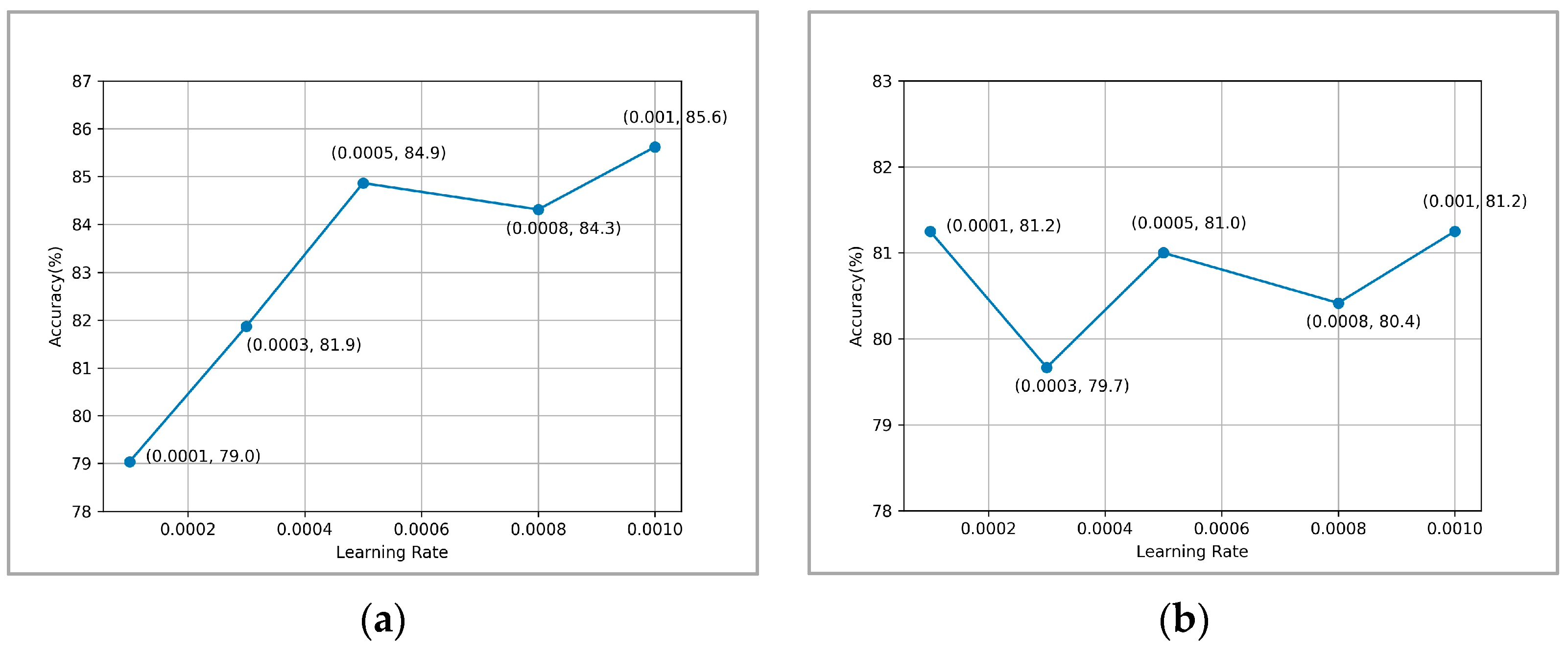Section 4 introduces the data set and experimental parameter selection process used to verify the feasibility of this method. Section 5 shows the experimental results of this paper and analyzes the experimental results. Section 6 demonstrates the performance of the proposed model in practical applications, including the model’s interpretability, generalization, real-time performance, and robustness. Section 7 summarizes the work of this paper and looks forward to related future work.

2. Related Work

2.1. Speech Emotion Recognition (SER)

Speech emotion recognition refers to analyzing a given speech signal to classify the signal into emotional categories. Common emotion categories usually include happiness, anger, sadness, calm, etc. Some existing research focuses on the processing of the speech signal itself, such as Mishra et al. [11], which aimed at modeling speech emotional features and used the MFCC coefficient matrix to calculate the MFCC-based spectral entropy and approximate entropy to improve the accuracy of emotion classification. Huang and Shen [12] applied the fractional Fourier transform (FrFT) to extract MFCC and combined it with a long short-term memory (LSTM) network for speech emotion recognition. Since the performance of FrFT depends on the transformation order $p$, the ambiguity function is used to determine the optimal order of each frame of speech, and the MFCC is extracted for each frame of speech under the optimal order of FrFT. Singh et al. [13] proposed a modulation feature extraction technology using a constant-Q filterbank based on human auditory-cortical physiology, which improved the model’s low-frequency resolution of speech signals.

Some researchers focus on the construction of SER models and are committed to cutting out the feature extraction link in the traditional speech emotion recognition process. For example, Kumar et al. [14] are based on the Residual Neural Network (ResNet) architecture and use triplet loss and cosine similarity to let the model learn emotional embedding so that it can recognize speech emotions. Shen et al. [15] proposed a parameter-free and flop-free time shift module, and combined this module with CNN, Transformer, and LSTM to conduct experiments, respectively, to promote channel information mixing in the SER pre-training task. Results on the IEMOCAP dataset are 74.8%, 74.7%, and 74.5%, respectively.

2.2. Multi-Task Learning for Speech Emotion Recognition

Multi-task learning methods were early used to solve tasks with less annotated data. They usually refer to training at least two related tasks together and then improving the main task by sharing parameters [16]. In multi-task learning models with speech emotion recognition as the main task, gender recognition, text information, and language information in speech are usually used as auxiliary tasks.

Han et al. [17] proposed an end-to-end emotion recognition method that integrates the automatic speech recognition (ASR) model and the SER model. This method combines features extracted from the ASR model with acoustic features and inputs them into the SER model, achieving an accuracy of 69.67% on the IEMOCAP dataset. Ma and Wang [18] proposed an interpretable multi-task shared feature learning (MSFL) model with language recognition as an auxiliary task. The model uses three language corpora (German, Chinese, and English) to train the model, and the results showed that MSFL outperformed most state-of-the-art models.

2.3. Soft Decision Tree

Soft decision trees generally refer to gradient-based decision trees that use differentiable functions for segmentation [19]. The branch structure of a common soft decision tree is shown in Figure 1.

Figure 1. Internal node construction of soft decision trees. The internal nodes of the soft decision trees are usually binary trees. According to certain rules, the probability $p$ of the feature being assigned to the left child node is calculated, and then $1-p$ is used to calculate the probability that the feature is assigned to the right child node.

With the development of deep learning and faced with the increasingly large number of parameters in deep learning models, researchers have begun to devote themselves to designing some lightweight and interpretable models. Good interpretability is a major advantage of soft decision trees, which has also prompted some researchers to combine artificial neural networks with soft decision trees. Wan et al. [20] proposed a Neural Supported Decision Tree (NBDT) model that uses a neural network such as ResNet18 as the backbone and replaces the final linear layer with a sequence of differentiable decision trees. The model was finally verified on the CIFAR and ImageNet datasets, and the accuracy increased by 2% compared with the original model. Among them, the CIFAR and ImageNet data sets are both computer vision data sets and are commonly used to evaluate classification, localization, and detection tasks in computer vision. Hehn et al. [21] combined CNN with decision trees; CNN was used to segment features, and decision trees were used to classify features. In order to improve the interpretability of the model, the model introduced a hyperparameter $\gamma$ to control the steepness of the probabilistic segmentation function, built a final decision tree on the International Symposium on Biomedical Imaging (ISBI) dataset, and used the decision tree to predict the test data.

In the field of speech emotion recognition, soft decision trees are rarely used. In a related field, Ji Teng and Seki Ling [22] used the original soft decision tree structure to achieve speech recognition of digit pronunciation in American English under noisy conditions and performed bottom-up pruning on the results. The two later implemented DT-based acoustic models (DTAMs) in 2012 [23] that can share training data that change little in context by modeling gender- and context-dependent acoustic spaces.

3. Methodology

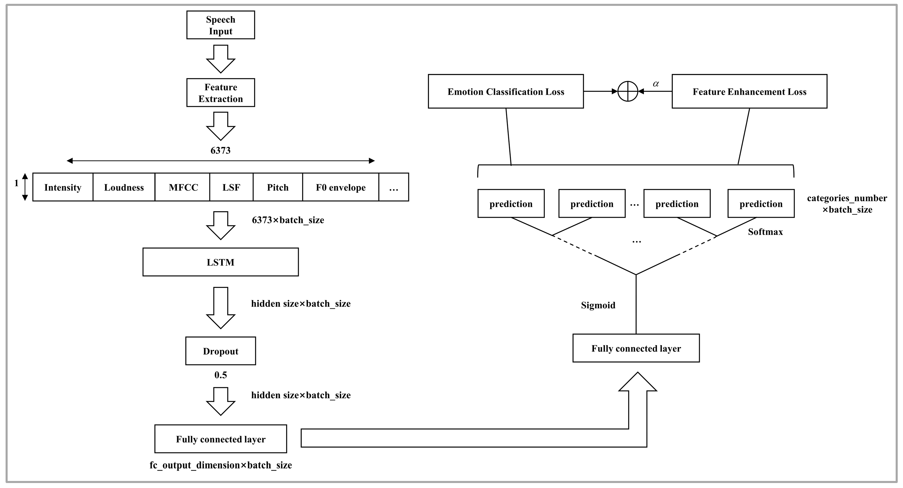
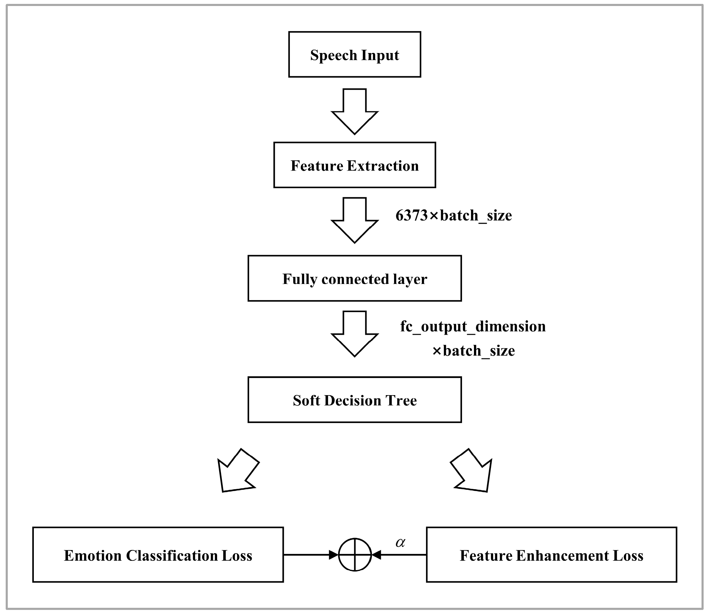
In this paper, we propose a multi-task learning framework to complete the speech emotion recognition task, as shown in Figure 2. The framework takes the original speech signal as input and extracts audio features of length 6373 using Opensmile’s IS13_ComParE [24] feature set. These features fully represent the acoustic properties of the speech signal.

Figure 2. The proposed model architecture.

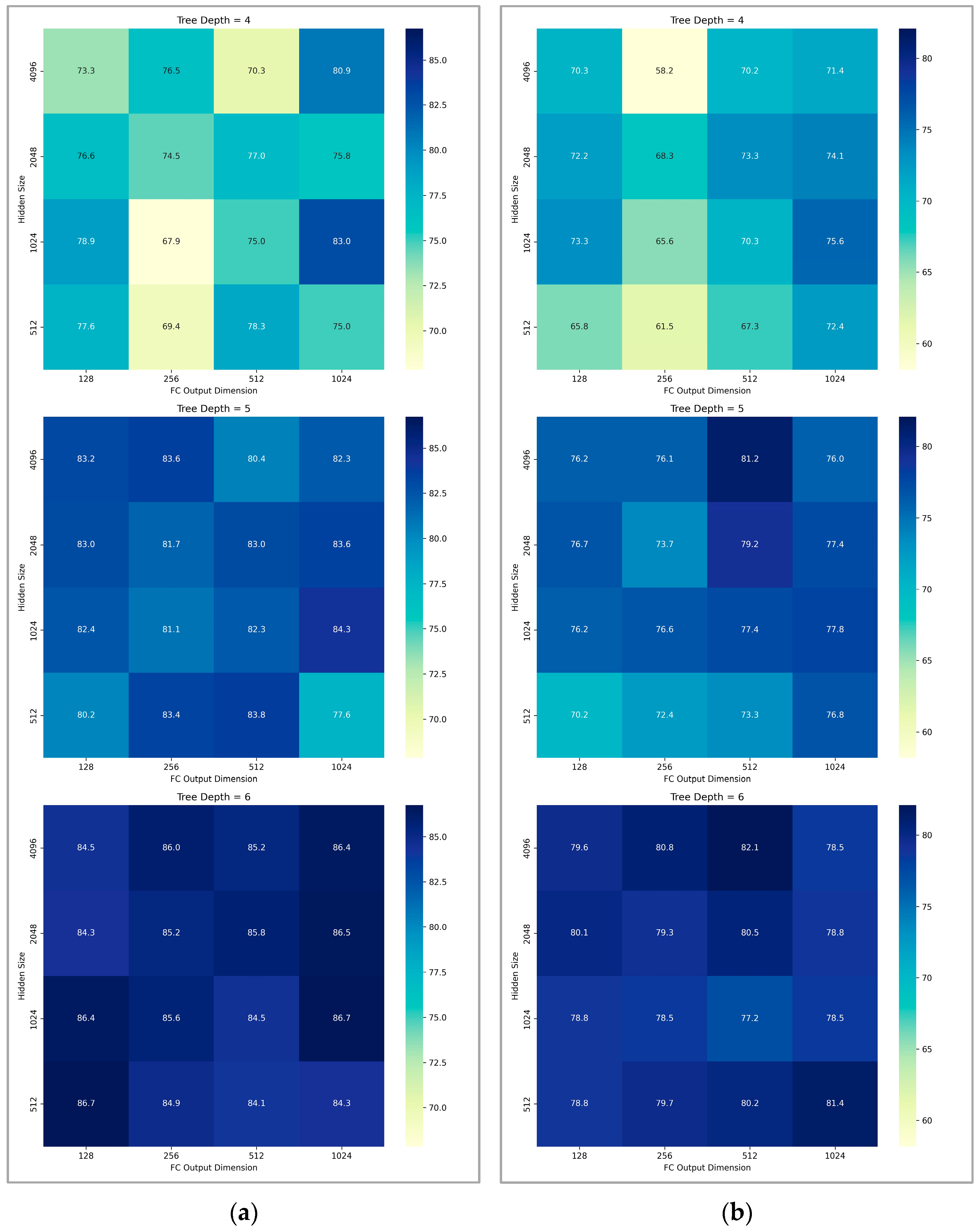
The extracted audio features are then fed into a one-layer LSTM model with a hidden dimension denoted as hidden_size. In our preliminary experiments (Section 4.2), we compared various values for hidden_size (e.g., 512, 1024, 2048, and 4096) to determine the optimal setting.

The LSTM model structure at a certain moment $t$ is shown in Figure 3.

Figure 3. LSTM network structure.

The functions involved in the LSTM model are as follows:

$$\left\{\begin{array}{l}{h}_t=o_t\ast \tanh c_t\hfill \\ c_t=f_t{c}_{t-1}+i_t\ast \tanh \left(w[x_t,h_{t-1}]+b\right)\hfill \\ o_t=sigmoid\left(w_o[x_t,h_{t-1}]+b_o\right)\hfill \\ f_t=sigmoid\left(w_f[x_t,h_{t-1}]+b_f\right)\hfill \\ i_t=sigmoid\left(w_i[x_t,h_{t-1}]+b_i\right)\hfill \end{array}\right.,$$

(1)

In the above equations, $x_t$, $h_t$, and $c_t$ are the input, output, and memory information of the LSTM network at moment $t$ respectively, $c_{t-1}$ and $h_{t-1}$ are the memory information and output of the previous moment, respectively. $o_t$, $f_t$, and $i_t$ are the output gate, forget gate, and input gate. $\ast$ indicates a multiplication operation.

After LSTM network learning and data enhancement, the output is connected to the fully connected layer, and the output dimension is represented as fc_output_dimension. The fully connected layer refines the learned features and then sends them to the soft decision tree for classification.

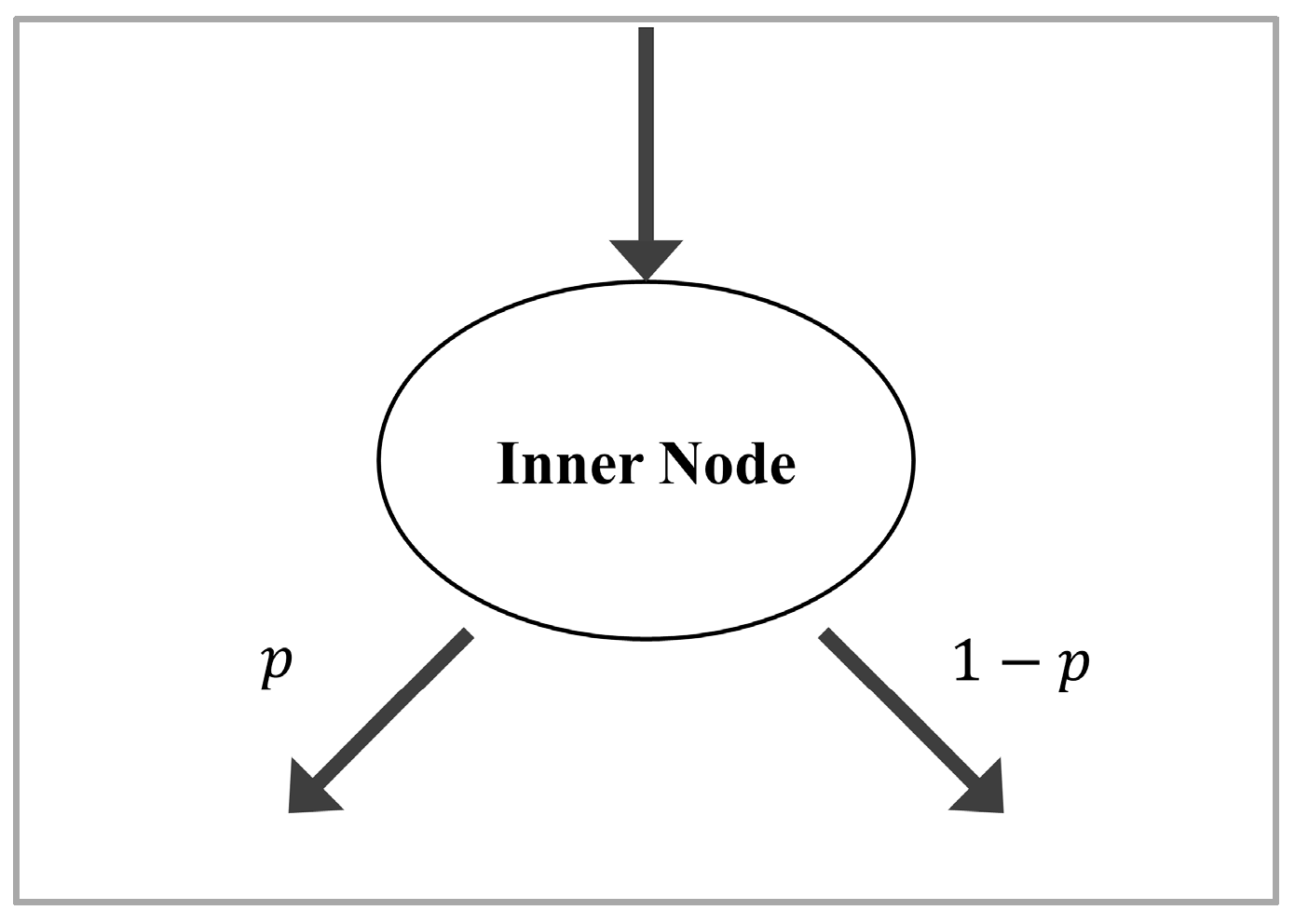
For the soft decision tree classification part, each internal node calculates the probability that the feature is divided into the left and right branches through Equation (2):

$$p\left(x\right)=\mathrm{sigmoid}\left(\beta \left(wx+b\right)\right),$$

(2)

where $p$ represents the probability value calculated by an internal node, $\omega$ and $b$ are the weight and bias of the node, respectively, and $\beta$ is the scaling factor. When $p$ is greater than 0.5, it goes to the left node, and when it is less than 0.5, it goes to the right node.

At the end of the model, we use two loss functions to perform the SER task and the SFE task, respectively. The SER task is a supervised task, and the loss is calculated based on the data label. The specific calculation requires first using Equation (3) to calculate the probability distribution $Q$ of each leaf node:

$$Q=\mathrm{softmax}\left(para{m}_{1,j}\right)$$

(3)

where $param$ is a trainable tensor with shape $1\times j$.

The difference between $Q$ and the true label distribution is then calculated using the cross-entropy loss function shown in Equation (4):

$$L_{SER}=-{\displaystyle \sum _{l\in LeafNodes}{p}^l}{\displaystyle \sum _{k\in batch\_size}{y}_k}\log \left(Q_k^l\right)$$

(4)

where $y$ is the true label distribution and $p$ is the probability of the input feature reaching the leaf node $l$.

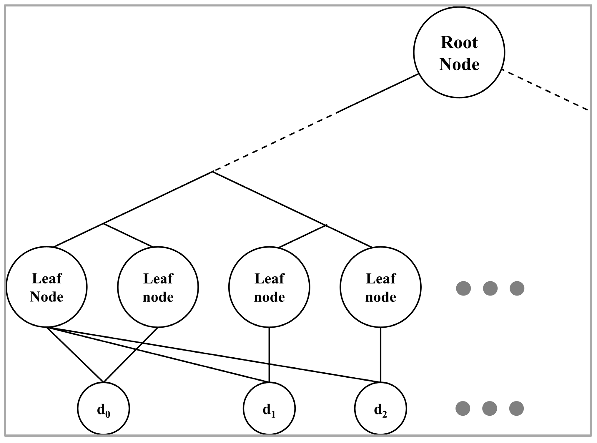
The SFE is an unsupervised task that calculates the loss function based on the distance between leaf nodes after soft decision tree classification. The distance relationship between leaf nodes is shown in Figure 4.

Figure 4. The distance relationship between leaf nodes.

Specifically, we calculate the distance between features in different leaf nodes to create a feature space that better separates different emotions. This process helps capture the subtle differences in speech patterns associated with different emotions, thus improving the model’s performance.

The goal of the SFE task is to minimize the distance between leaf nodes of the same parent node and maximize the distance between leaf nodes of different parent nodes. This is achieved by first calculating the distance between each anchor node feature and its adjacent node features, then subtracting this distance from the distance between the anchor node and other leaf nodes. The resulting values are then summed. This process is formalized in Equation (5):

$$L_{SFE}={\displaystyle \sum _{\mathrm{i}=1}^N\left({\displaystyle \sum _{a\in A_i}d\left(x_i,a\right)-}{\displaystyle \sum _{o\in O_i}d\left(x_i,o\right)}\right)}$$

(5)

where $N$ refers to the total number of leaf nodes in the soft decision tree, $d\left(x_i,a\right)$ is the distance between the anchor node $x_i$ and its adjacent leaf node $a$, and $d\left(x_i,o\right)$ is the distance between $x_i$ and other leaf nodes $o$. $A_i$ and $O_i$ denote the sets of adjacent nodes and other nodes for the anchor node $x_i$, respectively.

The distance $d\left(x,z\right)$ is calculated using the 2-norm equation:

$$d\left(x,z\right)={‖x-z‖}_2$$

(6)

where $x$ is the anchor node and $z$ is another leaf node.

Finally, we introduce a hyperparameter $\alpha$ to combine Equations (4) and (5) into a loss function:

$$L=\left(1-\alpha \right)L_{SER}+\alpha L_{SFE}$$

(7)

where $L_{SER}$ is the loss function for the speech emotion recognition task as defined in Equation (4), and $L_{SFE}$ is the loss function for the speech feature extraction task as defined in Equation (5). $\alpha$ is used to balance the two components of the total loss function.

4. Data Set and Experimental Parameter Selection

4.1. Data Set

We use two different language speech emotion data sets, CASIA (Chinese Academy of Sciences, Institute of Automation), and EMO-DB (Berlin Emotional Database) to verify the validity of the model.

This paper uses the CASIA public version [25]. This dataset is a Chinese emotion corpus constructed by the Institute of Automation, Chinese Academy of Sciences. It contains six emotions (happiness, sadness, anger, fear, surprise, and neutral), with 200 data points for each emotion, for a total of 1200 data points. The dataset was recorded by two men and two women in an environment with a signal-to-noise ratio of about 35 dB. It contains 500 different texts and is stored in PCM format with a sampling rate of 16,000, 16 bits, and 16-bit.

EMO-DB [26] is a German speech emotion database produced by the Technical University of Berlin. It was recorded by actors (5 men and 5 women) aged between 21 and 35 in an anechoic chamber environment. It contains 10 texts (5 long and 5 short) and 7 emotions (neutral, anger, afraid, happiness, sadness, disgusted, and bored). It contains a total of 535 data, including 233 male emotional speech and 302 female emotional speech. The duration of the data ranges from 1.2 s to 9.0 s.

4.2. Experimental Parameter Selection

Before conducting experiments, we selected and adjusted the key parameters of the model to ensure optimal performance across different datasets. Considering the size of the dataset, for the EMO-DB dataset, each experiment’s result is based on the average accuracy obtained through ten-fold cross-validation. For the CASIA dataset, each experiment’s result is based on the average accuracy obtained through five-fold cross-validation.

4.2.1. Model Parameter Selection

We discovered that the hidden dimension of the LSTM layer (hidden_size) variable is related to the fully connected layer’s output dimension (fc_output_dimension) and the depth of the soft decision tree (tree depth) because these parameters collectively influence the model’s capacity and its ability to capture and represent complex patterns in the data. Specifically, hidden_size affects the LSTM’s ability to store information over time, fc_output_dimension determines the feature representation power before classification, and tree depth controls the complexity of decision boundaries in the soft decision tree. Therefore, to thoroughly investigate their combined effects on model performance, we conducted experiments at tree depths of 4, 5, and 6, using hidden_size values of 512, 1024, 2048, and 4096, and fc_output_dimension values of 128, 256, 512, and 1024. The rest of the experimental parameter settings are shown in Table 1.

Table 1. The initial values of the remaining experimental parameters.

Parameter	Value
batch_size	128
epoch	100
learning rate	0.001
dropout	0.5
optimizer	adam
$\alpha$	0.5

Figure 5 shows the accuracy confusion matrices generated by these parameter combinations on the CASIA and EMO-DB datasets. The color intensity represents the accuracy levels. From the results, we observe that as the depth of the decision tree increases, the overall accuracy of the model improves for both datasets. This suggests that deeper trees allow for more complex decision boundaries, which enhances the classification performance of the model.

Figure 5. Accuracy confusion matrices for combinations of hidden_size and fc_output_dimension at different tree depths: (a) EMO-DB, (b) CASIA.

In addition, while there is no clear trend that larger hidden_size or fc_output_dimension consistently improves accuracy, some combinations produce higher performance (dark areas), and the impact of these parameters differs between CASIA and EMO-DB, highlighting the importance of dataset-specific tuning of parameters.

We observed that on the EMO-DB dataset, the highest accuracy of 86.7% can be achieved when the model’s (hidden_size, fc_output_dimension) is (512, 128) and (1024, 1024), respectively. Considering the training speed, memory and computing resources, model complexity, and other factors, we selected (512, 128) as the parameter for subsequent experiments on the EMO-DB dataset. Similarly, we found that on the CASIA dataset, the highest accuracy of 82.1% can be achieved when the model’s (hidden_size, fc_output_dimension) is (4096, 512). Therefore, we selected (4096, 512) as the parameter for subsequent experiments on the CASIA dataset.

4.2.2. Hyperparameter Selection

Based on the above, we experiment with the learning rate and the parameter $\alpha$ in Equation (7).

The learning rate is a key hyperparameter for training neural networks because it determines the step size of each iteration while moving towards the minimum value of the loss function. We tried five different learning rates: 0.0001, 0.0003, 0.0005, 0.0008, and 0.001. Each learning rate was tested under the same conditions to evaluate its impact on the overall accuracy of the model, and the results are shown in Figure 6.

Figure 6. Experimental results at different learning rates: (a) EMO-DB, (b) CASIA.

Figure 6 illustrates that on the EMO-DB dataset, the accuracy corresponding to different learning rates ranges from 79% to 85.6%. With the increase in the learning rate, the accuracy exhibits continuous growth followed by a stable trend, reaching its peak of 85.6% at a learning rate of 0.001. On the CASIA dataset, the accuracy corresponding to different learning rates ranges from 79.7% to 81.2%, reaching a peak of 81.2% when the learning rates are 0.001 and 0.0001. Considering factors such as model complexity and training efficiency, we selected 0.001 as the learning rate for training the model on the CASIA dataset in subsequent experiments.

To explore the optimal $\alpha$ value that balances the two loss functions $L_{SER}$ (Equation (4)) and $L_{SFE}$ (Equation (5)), we conducted experiments based on the above experiments. The experimental results are shown in Figure 7.

Figure 7. Experimental results at different $\alpha$ values: (a) EMO-DB, (b) CASIA.

We experimented with $\alpha$ values from 0 to 0.9 in increments of 0.1 to understand their impact on model performance. From Equation (7), it can be concluded that when the $\alpha$ value is small, the model tends to optimize $L_{SER}$, and when the $\alpha$ value is large, the model tends to optimize $L_{SFE}$.

On the EMO-DB dataset, the model’s accuracy reaches a maximum of 85% when the value of $\alpha$ equals 0.1, at which point $L_{SER}$ and $L_{SFE}$ achieve optimal balance. Subsequently, with an increase in the proportion of $L_{SFE}$, the accuracy shows a fluctuating downward trend. Similarly, on the CASIA dataset, the model’s accuracy reaches a maximum of 81.2% when the value of $\alpha$ is 0.1 and then shows a downward trend as the value of $\alpha$ increases. This indicates that the feature enhancement task can play a certain auxiliary role during model training but still cannot replace the dominant role of the speech emotion recognition task.

5. Evaluation Results

This chapter will introduce two baseline models and analyze in detail the experimental results of the baseline models and the experimental results of the method proposed in this paper. Then, a t-test and p-value calculation will be performed on the accuracy of each fold, and the unweighted accuracy (UA) will be calculated to compare with the methods in other papers.

5.1. Baseline Models Introduction

To evaluate the contribution of the LSTM layer, we designed a baseline model, as shown in Figure 8, in which the LSTM layer is removed while retaining other components in Figure 2.

Figure 8. Baseline model without LSTM layer.

Subsequently, to evaluate the effectiveness of $L_{SFE}$, we removed $L_{SFE}$ based on the baseline model in Figure 8, as illustrated in Figure 9.

Figure 9. Baseline model without LSTM layer and $L_{SFE}$.

5.2. Analysis of Experimental Results

To validate the effectiveness of the proposed method, we trained two baseline models and the proposed method on the CASIA and EMO-DB datasets. The parameter settings referenced the experiments in Section 4.2, as shown in Table 2. In particular, the baseline model without the LSTM layer does not use the hidden_size parameter, and the baseline model without the $L_{SFE}$ has an $\alpha$ value of 0.

Table 2. The experimental parameter settings.

Parameter	EMO-DB	CASIA
batch_size	128
epoch	200
learning rate	0.001
dropout	0.5
optimizer	adam
tree_depth	6
$\alpha$	0.1
hidden_size	512	4096
fc_output_dimension	128	512

5.2.1. Confusion Matrix Analysis

In Figure 10, we present the confusion matrices of the experimental results for the two baseline models and the proposed model in a fold. These matrices illustrate the performance differences between the models and provide a detailed view of their classification accuracy across different categories.

Figure 10. Confusion matrix of baseline experiment results: (a) EMO-DB—w/o LSTM and $L_{SFE}$, (b) CASIA—w/o LSTM and $L_{SFE}$, (c) EMO-DB—w/o LSTM, (d) CASIA—w/o LSTM, (e) EMO-DB—w/LSTM and $L_{SFE}$, (f) CASIA—w/LSTM and $L_{SFE}$.

From Figure 10, it can be observed that in the EMO-DB dataset, the introduction of the SFE component significantly reduces the confusion of the model between similar emotions such as happiness and anger, neutral and boredom, and neutral and happiness, thereby improving the overall accuracy of the model. In the CASIA dataset, the SFE component significantly reduces the confusion between fear and sadness. Although the accuracy of some categories decreases slightly after the introduction of the SFE component (e.g., anger in EMO-DB and anger and surprise in CASIA), the classification performance of other categories improves significantly overall. This indicates that the SFE component reduces the confusion between emotions to a certain extent.

Compared with the two baseline models, our proposed model shows the best performance on various emotion categories, which shows that LSTM can effectively capture time series features, while $L_{SFE}$ helps to enhance speech emotion features.

5.2.2. Accuracy Curve Analysis

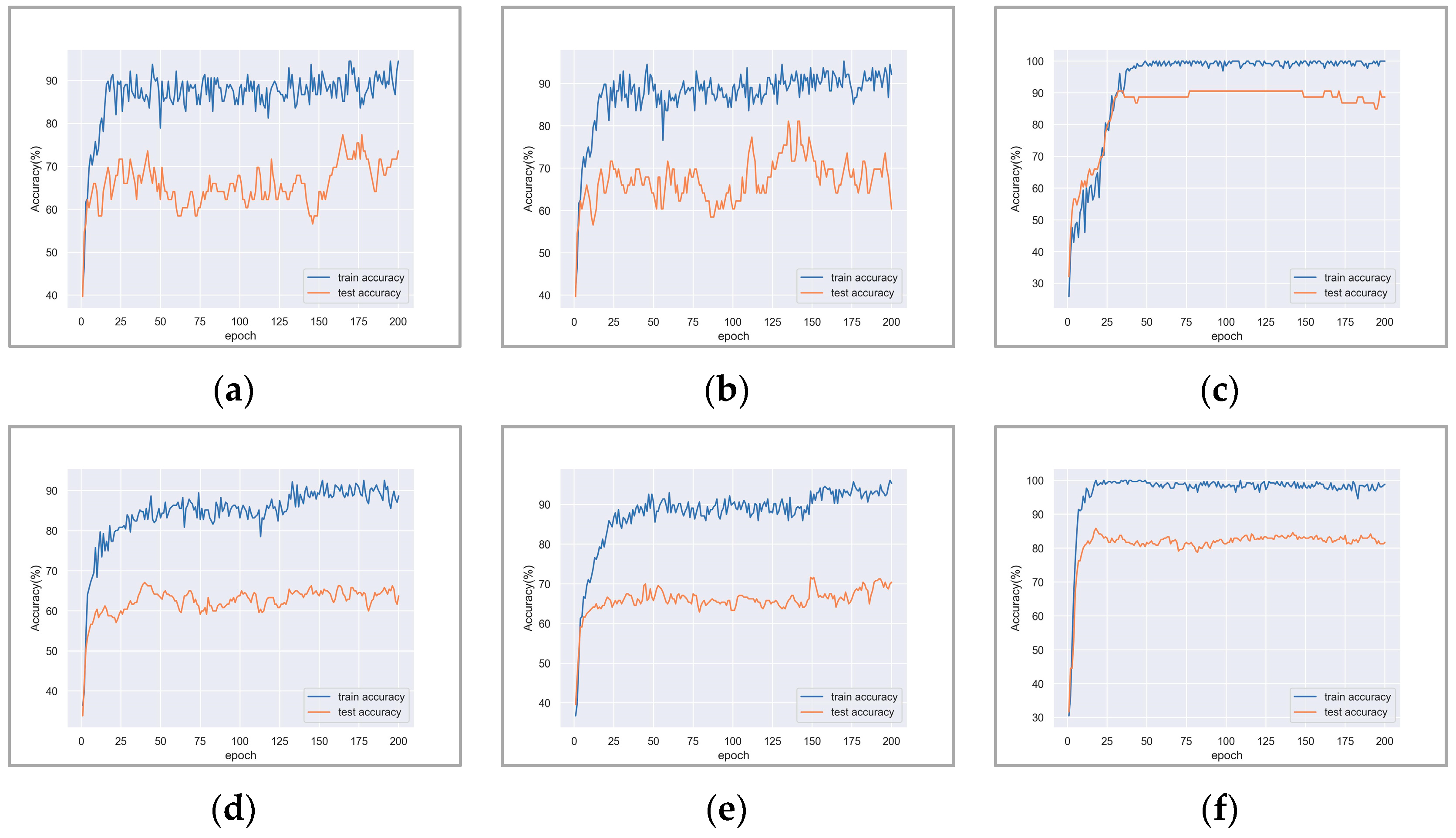
In Figure 11, we present the accuracy curves of the two baseline models and the proposed model in the experiment. Each curve shows the changes in training accuracy and test accuracy, thereby evaluating the generalization performance, convergence speed, and overfitting of the model.

Figure 11. Baseline experiment accuracy curve: (a) EMO-DB—w/o LSTM and $L_{SFE}$, (b) CASIA—w/o LSTM and $L_{SFE}$, (c) EMO-DB—w/o LSTM, (d) CASIA—w/o LSTM, (e) EMO-DB—w/LSTM and $L_{SFE}$, (f) CASIA—w/LSTM and $L_{SFE}$.

Through experiments on the EMO-DB and CASIA datasets, we found that adding $L_{SFE}$ improved the model’s test accuracy on the datasets, indicating enhanced generalization ability and alleviation of overfitting. Compared to the two baseline models, our proposed model showed significantly faster convergence during training, with stable accuracy after convergence. This suggests that the model, with the incorporation of LSTM and $L_{SFE}$, can learn features and patterns from data more efficiently, exhibiting superior learning and generalization capabilities, resulting in higher efficiency and stability in handling speech emotion recognition tasks.

5.3. Comparative Analysis

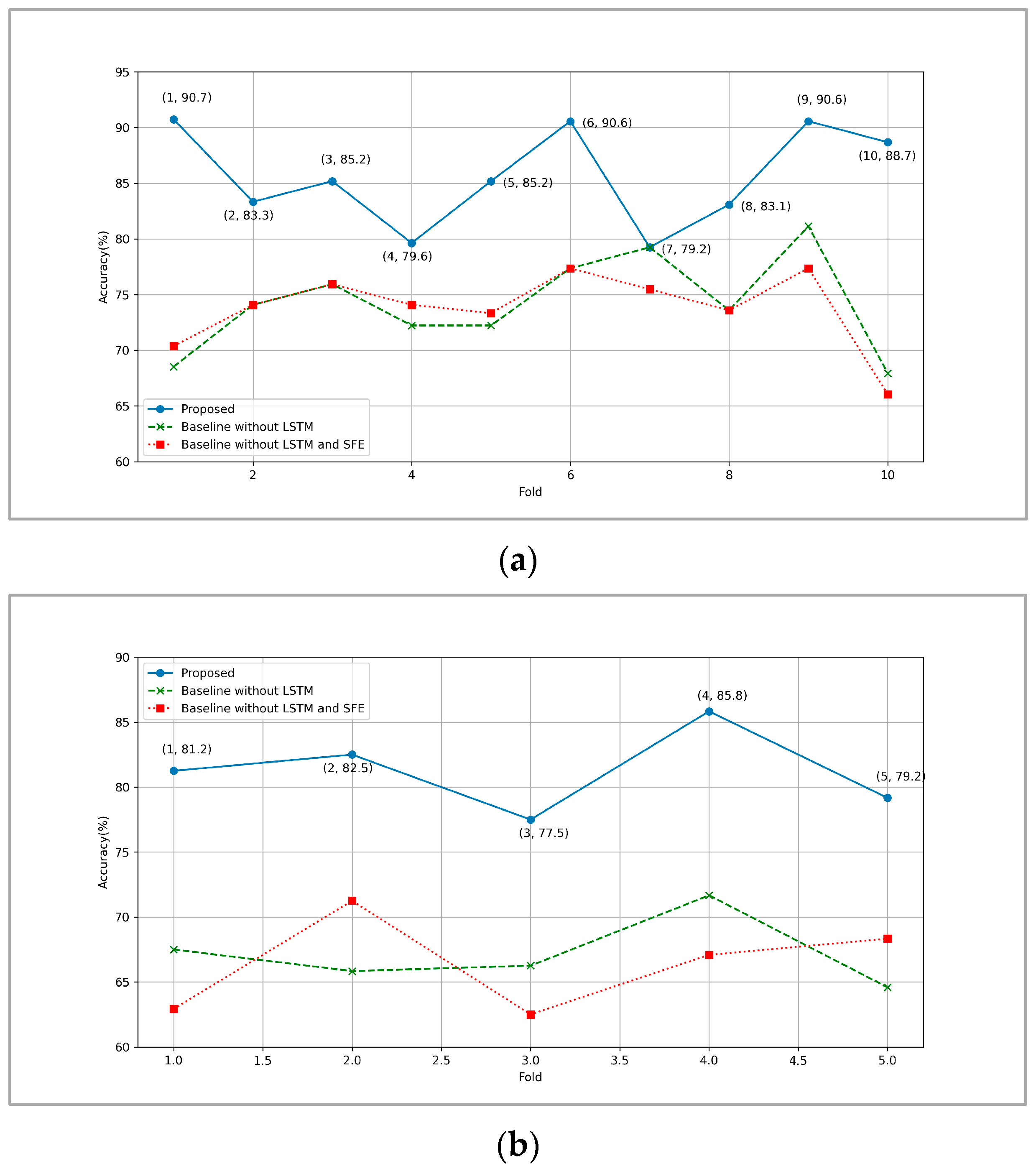
In this section, we first compared the accuracy of two baseline models and the proposed model in each fold (Figure 12) and calculated the accuracy rates for all three models (Table 3). To validate the effectiveness of the proposed method, we conducted a t-test and calculated the p-value between the experimental results of one baseline model and the proposed method (Table 4).

Figure 12. Comparison of experimental results between the baseline models and the proposed method: (a) EMO-DB, (b) CASIA.

Table 3. UA comparison between the baseline models and the proposed method.

Model	EMO-DB (%)	CASIA (%)
$\mathrm{w}/\mathrm{o} \mathrm{LSTM} \mathrm{and} L_{SFE}$	73.8	66.4
w/o LSTM	74.2	67.2
proposed	85.6	81.3

Table 4. Comparative analysis of the proposed model against the baseline.

Corpus	Model	t-Value	p-Value	Significance
EMO-DB	Proposed vs. Baseline	5.9	7.4 × 10−6	Yes
CASIA	Proposed vs. Baseline	6.8	7.1 × 10−5	Yes

From Figure 12, it is evident that the proposed model significantly outperforms the two baseline models on both datasets. Specifically, on the EMO-DB dataset, the accuracy of the proposed model exceeds 85% in most folds, with some folds even surpassing 90%. In contrast, the baseline model without the LSTM module shows accuracy fluctuations between 70% and 85%, indicating a clear underperformance compared to the proposed model. For the baseline model without both the LSTM module and the $L_{SFE}$, the accuracy hovers around 75%, with the best folds reaching only up to 80%.

On the CASIA dataset, the proposed model continues to demonstrate superior performance, with most folds achieving accuracies above 80% and the best fold reaching 85.8%. In comparison, the baseline model without the LSTM module shows accuracy fluctuations between 65% and 75%. The baseline model without both the LSTM module and the $L_{SFE}$ has accuracies ranging from 60% to 75%, with considerable variation and two folds falling below 65%.

These results further illustrate the critical importance of the LSTM module and the $L_{SFE}$ in enhancing the performance of the proposed model in emotion recognition tasks.

Based on the data from Figure 12, we calculated the UA of each model on both datasets, and the results are recorded in Table 3. It is evident that the proposed model outperforms the baseline models on both datasets. The baseline model without the LSTM module performs slightly better than the baseline model without both the LSTM module and the $L_{SFE}$, indicating that the $L_{SFE}$ contributes to improving the model’s performance to some extent.

To ensure a rigorous comparison between our proposed model and the baseline, we conducted a t-test, a statistical method commonly employed to assess the significance of differences in mean performance between two models [27]. This analysis involved calculating the p-value from the t-value, with statistical significance typically defined at the 0.05 level. The equation used for the t-test is as follows:

$$\mathrm{t}=\frac{{\overline{X}}_{baseline}-{\overline{X}}_{new}}{\sqrt{\left(s_{baseline}^2+s_{new}^2\right)/n}}$$

(8)

Among them, ${\overline{X}}_{baseline}$ and ${\overline{X}}_{new}$ are the average accuracy of the baseline model and the new method, respectively, ${\mathrm{s}}_{baseline}$ and ${\mathrm{s}}_{new}$ are their respective standard deviations, and $n$ is the number of samples.

Following this, we formulated a one-tailed hypothesis, with the null hypothesis (H0) positing that the proposed model’s performance is not significantly greater than or equal to that of the baseline and the alternative hypothesis (H1) suggesting the opposite.

Subsequently, to thoroughly evaluate the effectiveness of our proposed model, we selected a baseline model excluding LSTM and $L_{SFE}$ components and conducted a t-test against our model. This comprehensive analysis was facilitated using the ‘stats’ function of the ‘scipy’ library in Python, enabling the computation of both t-values and p-values. The results of these calculations are presented in Table 4.

From Table 4, it can be observed that our proposed model demonstrates significant performance advantages over the baseline model in both the EMO-DB and CASIA datasets. Specifically, in the EMO-DB dataset, our model yielded a t-value of 5.9, corresponding to a p-value of 7.4 × 10⁻⁶, with a significance of ‘Yes’. Similarly, in the CASIA dataset, our model obtained a t-value of 6.8, with a corresponding p-value of 7.1 × 10⁻⁵, also indicating significance. These findings further support our research hypothesis, indicating that our proposed model outperforms the baseline model significantly across these two datasets.

5.4. Comparison with Other Studies

Table 5 shows the comparison between this paper and other studies using UA result evaluation. All experiments use the corresponding data sets and indicate the corresponding verification folds.

Table 5. Comparison with other methods.

Corpus	Methods	Folds	UA (%)
CASIA	Bi-A2CEmo [28] (2024)	5-fold	80.4
	ShiftLSTM [15] (2024)	5-fold	66.5
	Cascaded Attention Network [29] (2024)	10-fold	67.1
	proposed	5-fold	81.3
EMO-DB	Bi-A2CEmo [28] (2024)	5-fold	80.2
	CQT-MSF + DNN-SVM [13] (2023)	5-fold	76.2
	MFMC + DNN [30] (2023)	5-fold	84.7
	proposed	10-fold	85.6

In Table 5, Li et al. [28] proposed a deep learning framework capable of simultaneously mapping and inverting acoustic and phonetic signals. This framework uses a feature dimension adaptive mechanism, allowing the model to adaptively allocate matrix weights. This results in a better understanding of the distribution of real features and generates high-precision mapping features, thereby improving the accuracy of speech emotion recognition. Liu et al. [29] proposed a speech emotion recognition architecture that integrates a cascaded attention network and an adversarial loss strategy. The cascaded attention network combines spatio-temporal attention and head-fusion self-attention to pinpoint target emotional regions within speech segments. The adversarial joint loss strategy enhances the intra-class compactness and inter-class separability of the learned features. Mishra et al. [30] used speech features extracted by Mel-Frequency Magnitude Coefficient (MFMC) as the input of a Deep Neural Network (DNN) classifier for the speech emotion recognition task, where MFMC is a modified version of MFCC, which replaces the first magnitude of the Discrete Fourier Transform (DFT) with the square of the magnitude and adds a discrete cosine term.

It can be seen that our proposed method performs well on the CASIA and EMO-DB corpora and achieves a higher UA percentage compared to existing methods. This shows the effectiveness and potential of our proposed method for emotion recognition tasks.

6. Performance Evaluation

In this chapter, we will evaluate the performance of the proposed model, including feature visualization analysis, interpretability analysis of the soft decision tree, generalization analysis, real-time performance analysis, and performance analysis in noisy environments.

6.1. Visualization Analysis

6.1.1. Feature Visualization Analysis

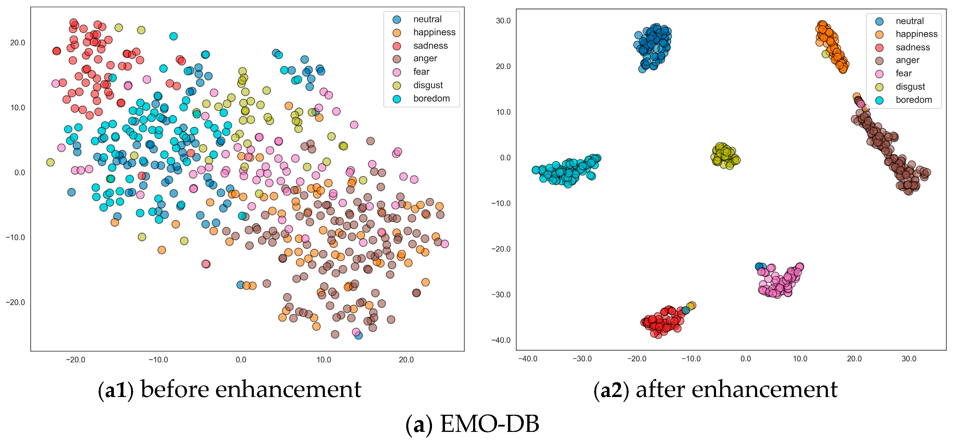
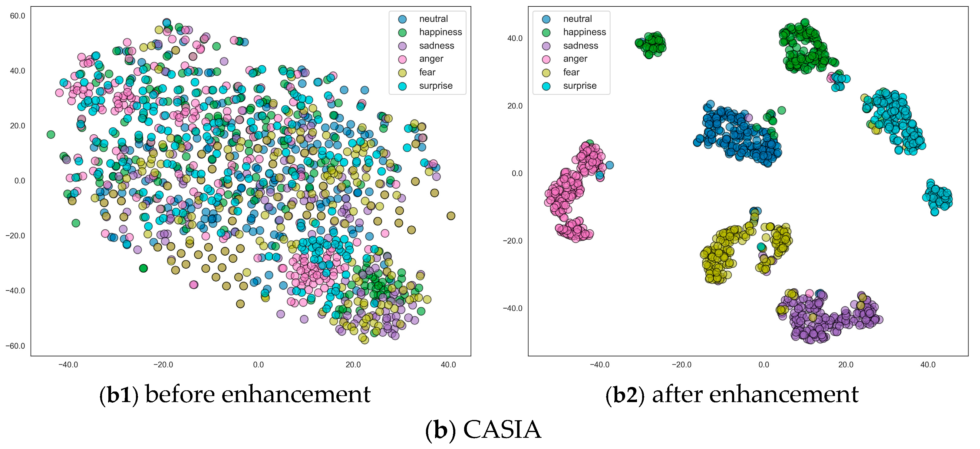
We employ t-Distributed Stochastic Neighbor Embedding (t-SNE) to visualize the feature distributions before and after feature enhancement, as shown in Figure 13. t-SNE is a dimensionality reduction technique that is particularly well-suited for visualizing high-dimensional data by converting similarities between data points into joint probabilities and minimizing the Kullback–Leibler divergence between the joint probabilities of the low-dimensional embedding and the high-dimensional data [31]. The t-SNE method helps us gain insights into how the features evolve during the training process and how well the model is able to distinguish between different emotional categories.

Figure 13. Feature distributions before and after feature enhancement.

It can be observed that for the EMO-DB dataset, the raw features before enhancement show significant overlap between different emotional categories, indicating that the model has not yet learned to distinguish emotions at this stage. After feature enhancement, the emotional categories become clearer and better separated, indicating that the model has effectively learned to distinguish emotions in the EMO-DB dataset. There is a slight confusion between anger and happiness, which may be because both emotions can have high-pitched and lively tones and fast speech rates. Similarly, some neutral samples are placed in the fear cluster because certain low-pitched neutral samples closely resemble the expression of fear, resulting in significant overlap in the feature space.

For the CASIA dataset, the features before enhancement show a very dispersed distribution with significant overlap between different emotional categories, indicating a lack of initial discriminative ability. After enhancement, the features for each emotional category become more clustered and distinctive, indicating that the model has effectively learned and distinguished the emotional categories in the CASIA dataset. However, there is still some confusion between emotions, such as fear and sadness, which may be due to both emotions having low and oppressive tones. Additionally, some happiness samples are placed in the neutral cluster, possibly because certain less intense happiness emotions are closer to neutral emotions, leading to confusion.

6.1.2. Decision Tree Visualization

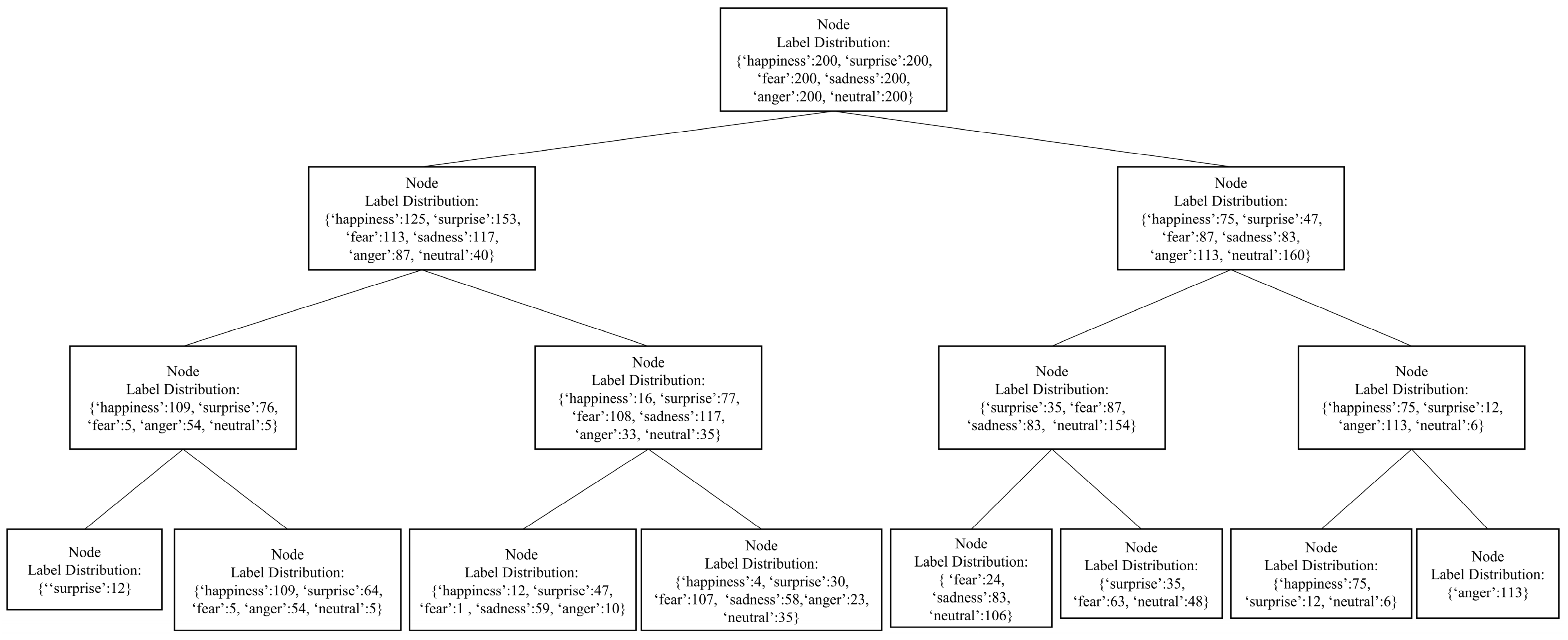
In this section, we visualize the generated soft decision tree using a specific fold of the model trained on the CASIA dataset to gain deeper insights into how the model makes classification decisions based on different emotion categories, analyzing the interpretability of the proposed model.

Figure 14 depicts the first four layers of the binary soft decision tree, where each node contains the label distribution of emotions. Due to space constraints, only these four layers are shown, although the complete model consists of six layers. This visualization highlights the model’s process of refining its classification decisions at each level.

Figure 14. Decision tree visualization of the model using the CASIA dataset.

The root node starts with an equal distribution of all six emotions, each with 200 samples: happiness, surprise, fear, sadness, anger, and neutral. At the first split, the tree branches into two nodes, each showing distinct distributions of emotions. The left node has a higher concentration of happiness and surprise, indicating the model’s initial attempt to separate these emotions. The right node shows a mix of all emotions, with notable amounts of fear, sadness, and neutral emotions.

The second level further refines the emotion distributions. In the left subtree, happiness and surprise become more dominant, with nodes showing distinct separations. The right subtree continues to mix emotions, highlighting nodes with high concentrations of fear, sadness, and neutral emotions. The third and fourth levels continue to refine the distributions. Nodes in the left subtree show a clearer separation of happiness and surprise, with some nodes exclusively containing a single emotion. The right subtree highlights the challenges in separating fear, sadness, and neutral, with nodes showing mixed distributions.

The soft decision tree visualizes the model’s ability to gradually separate different emotions. Early splits focus on broad distinctions, while deeper nodes refine these distinctions for more specific emotions. This illustrates that using LSTM for feature extraction and calculating distances between leaf nodes enhances the model’s ability to differentiate subtle emotional cues, leading to more precise classification. Additionally, the decision tree highlights areas where emotions are harder to separate. For example, nodes with mixed distributions of fear, sadness, and neutral suggest overlapping features, making them challenging to distinguish.

By examining the paths from the root to the leaf nodes, we can trace the model’s decision-making process. This traceability enhances interpretability by showing how the model classifies emotions, revealing the strengths in distinguishing certain emotions and the challenges in separating others, effectively demonstrating the model’s interpretability and performance.

6.2. Generalization Analysis

In this section, we evaluate the generalization ability of our proposed model through cross-corpus experiments. We use three datasets (EMO-DB, CASIA, and IEMOCAP) to evaluate the generalization ability of the model to unseen data from different datasets. The parameters of the model trained using the IEMOCAP dataset are shown in Table 6, and the parameter acquisition steps are the same as in Section 4.2.

Table 6. The experimental parameter settings of IEMOCAP.

Parameter	IEMOCAP
batch_size	128
epoch	200
learning rate	0.001
dropout	0.5
optimizer	adam
tree_depth	5
$\alpha$	0.1
hidden_size	512
fc_output_dimension	128

The Interactive Emotional Binary Motion Capture (IEMOCAP) [32] database is a widely used dataset in emotion recognition research. Collected by the Signal Analysis and Interpretation Laboratory (SAIL) at the University of Southern California, it contains approximately 12 h of audiovisual data. The data were recorded by five male and five female actors, encompassing both scenario-based and script-based dialogues. Each audio segment has an average duration of 4.5 s and a sampling rate of 48 kHz. Every audio clip is annotated by at least 3 evaluators for emotional content, covering emotions such as neutral, excitement, sadness, and anger. The IEMOCAP database is an essential resource for evaluating emotion recognition models and is widely used in emotion recognition and human-computer interaction research.

Table 7 lists six cross-corpus experimental schemes and corresponding recognition tasks. Each task involves training the model on one dataset and testing the model on another dataset to evaluate its ability to generalize to different emotion datasets. Since the model in the C -> I and E -> I tasks has been changed to four classes, the number of training samples has significantly decreased. Therefore, we adjusted the height of the decision tree from 6 to 5.

Table 7. Six cross-corpus experimental schemes and identification tasks.

Task	Dataset (# Total Number)	Emotion Category (# Samples of Each Emotion)
E -> C, C -> E	CASIA (1000)	neutral (200), happiness (200), sadness (200), anger (200), fear (200)
	EMO-DB (408)	neutral (79), happiness (71), sadness (62), anger (127), fear (69)
I -> C, C -> I, I -> E, E -> I	CASIA (800)	neutral (200), happiness (200), sadness (200), anger (200)
	IEMOCAP (4936)	neutral (1708), excited (1041), sadness (1084), angry (1103)
	EMO-DB (339)	neutral (79), excited (71), sadness (62), anger (127)

To evaluate generalization performance, Table 8 provides the UA of the ablation models without LSTM and $L_{SFE}$, without LSTM, and the proposed model across six cross-corpus tasks. These tasks are labeled as C -> E, C -> I, E -> C, E -> I, I -> C, and I -> E. Each task represents different combinations of source and target corpora, where “C” stands for the CASIA corpus, “E” stands for the EMO-DB corpus, and “I” stands for the IEMOCAP corpus.

Table 8. UA of different ablation models in six cross-corpus schemes (%).

Task	C -> E	C -> I	E -> C	E -> I	I -> C	I -> E
$\mathrm{w}/\mathrm{o} \mathrm{LSTM} \mathrm{and} L_{SFE}$	40.5	45.2	31.7	44.6	44.5	52.9
w/o LSTM	40.5	45.2	31.8	44.7	44.4	54.7
proposed	44.1	45.8	34.1	46.7	46.9	59.3

The results indicate that the proposed model consistently outperforms the ablation models in most cross-corpus scenarios. This demonstrates the effectiveness of our model in generalizing to different datasets and emotional categories. Specifically, the proposed model shows a significant improvement in the I -> E (IEMOCAP to EMO-DB) task, achieving a UA of 59.3%, highlighting its robustness in recognizing emotions across different datasets. This is because the LSTM module excels at capturing temporal dependency features in speech signals, which helps in better understanding the emotional dynamics of the speaker. In contrast, models without LSTM perform weaker in handling emotion classification tasks involving complex temporal dependencies.

Regarding the SFE component, although its effect on UA improvement is not apparent in other tasks, in the I -> E task, the UA increased by 6.4% compared to the model without SFE, underscoring the importance of the SFE component. This might be because the IEMOCAP and EMO-DB datasets have substantial differences in recording environments, speakers, and emotional expression styles. The IEMOCAP dataset contains more diverse emotional expressions and a more varied range of speakers, while the EMO-DB dataset has more standardized emotional expressions. Therefore, the model faces greater challenges in the I -> E task, requiring stronger generalization capabilities.

From the above analysis, we can conclude that by incorporating LSTM and $L_{SFE}$, our model effectively captures temporal dependencies and enhances feature learning, leading to better generalization performance across various emotional datasets.

6.3. Real-Time Analysis

In this section, we evaluate the real-time performance of the proposed model by measuring the execution time required to process audio samples from the EMO-DB and CASIA datasets. This analysis is crucial for determining the model’s feasibility in real-world applications where prompt responses are essential.

The execution time is measured for each dataset, and the average execution time along with the standard deviation is presented in Table 9.

Table 9. Average execution time for each dataset and its standard deviation.

EMO-DB	Average execution time (s)	0.8
	Standard deviation (s)	0.1
CASIA	Average execution time (s)	6.0
	Standard deviation (s)	0.5

For the EMO-DB dataset, the model exhibits a low average execution time of 0.8 s with a standard deviation of 0.1 s. This indicates that the model can process audio samples from the EMO-DB dataset quickly and consistently, making it suitable for applications requiring rapid responses.

The average execution time for processing audio samples from the CASIA dataset is 6.0 s, with a standard deviation of 0.5 s. While this execution time is significantly higher compared to the EMO-DB dataset, it remains within an acceptable range for many real-time applications, although further optimization may be needed for time-sensitive tasks. This is largely due to the fact that the CASIA dataset has a larger number of samples and a longer average duration per sample compared to the EMO-DB dataset, leading to increased processing time.

6.4. Noise Environment Analysis

In this section, we evaluate the performance of the proposed model in noisy environments. The NOISEX-92 noise dataset [33] is utilized to add noise to the EMO-DB and CASIA datasets at different signal-to-noise ratios (SNRs) of 0 dB, 5 dB, and 10 dB. The NOISEX-92 noise dataset is a widely used collection of various noise recordings designed for testing and evaluating the performance of speech and audio processing systems under noisy conditions. The dataset includes 15 types of noise, such as babble, factory noise, white noise, and many more. These noises are representative of real-world environments, making them suitable for evaluating the robustness of speech emotion recognition systems. This paper uses 10 of these noises for experiments, which helps to understand the robustness of the model under various noisy conditions. The experimental results are presented in Table 10 and Table 11, and a visual example of the noise addition process is shown in Figure 15, where a speech sample labeled as “anger” from the EMO-DB dataset is mixed with babble noise.

Table 10. UA after mixing the CASIA dataset with noise.

CASIA
	babble	f16	factory1	factory2	leopard
0 db	71.9	71.4	72.8	73.7	70.5
5 db	73.1	72.8	73.8	74.4	72.8
10 db	75.7	75	74.5	75.9	73.6
	machinegun	pink	tank	volvo	white
0 db	72.2	71.4	74.0	74.5	75.1
5 db	73.5	74.2	75.5	75.4	77.3
10 db	74.9	75.3	77	76.8	77.9

Table 11. UA after mixing the EMODB dataset with noise.

EMO-DB
	babble	f16	factory1	factory2	leopard
0 db	77.0	80.7	75.9	81.9	80.2
5 db	81.5	84.1	80.0	84.1	83.6
10 db	84.3	85.4	82.6	86.2	84.1
	machinegun	pink	tank	volvo	white
0 db	82.3	78.7	81.9	82.6	80.7
5 db	83.9	80.8	82.6	83.4	82.3
10 db	84.3	83.2	84.5	83.8	83.2

Figure 15. An example of adding babble noise to an “anger” speech sample from the EMO-DB dataset. (a1–a5): spectrogram, (b1–b5): waveform, (a1,b1): original audio, (a2,b2): audio with SNR of 10 dB, (a3,b3): audio with SNR of 5 dB, (a4,b4): audio with SNR of 0 dB, (a5,b5): noisy audio.

The results of the noise environment analysis are summarized in Table 10 and Table 11. These tables show the UA for different types of noise added to the CASIA and EMO-DB datasets at 0 dB, 5 dB, and 10 dB SNRs.

For the CASIA dataset, at 0 dB SNR, the UA is lower across all noise types, indicating the challenge the model faces in extremely noisy environments. As the SNR increases to 5 dB and 10 dB, there is a noticeable improvement in UA across all noise types. The highest UA at 10 dB is observed with white noise (77.9%) and tank noise (77.0%). The results show that the model’s performance improves significantly with higher SNRs, demonstrating its ability to handle moderate noise levels.

Similar to the CASIA dataset, EMO-DB has low UA at 0 dB SNR, which improves with increasing SNR. The highest UA at 10 dB SNR is observed with f16 noise (85.4%) and factory2 noise (86.2%). The model shows robust performance even at lower SNRs, maintaining relatively high UA compared to CASIA, which may be attributed to the higher quality and clarity of the EMO-DB recordings.

Overall, babble noise, which simulates a background crowd, presents a challenging environment, especially at lower SNRs. The proposed model performs better with machine-generated noises (e.g., f16, factory2) as the SNR increases. White noise consistently shows higher UA across both datasets, indicating the model’s resilience to this type of noise. The results suggest that the model can be reliably used in real-world applications where background noise is prevalent.

7. Conclusions

In this paper, we first summarize some related works in speech emotion recognition, multi-task learning, and decision trees, then introduce the proposed model structure and loss function, and describe the datasets used in the experiment. Before the formal experiment, we explored the process of selecting model parameters on different datasets, discussed why different parameter values presented different experimental results, and finally determined two sets of parameter values for two datasets and conducted experiments. In the experimental phase, we constructed two baseline models to verify the feasibility of the proposed method in this paper. Then, we compared the experimental results of the proposed method with the baseline model and some recent work to prove the effectiveness of the proposed method. Additionally, to illustrate the interpretability of the proposed method, we visualized the features before and after enhancement and the final decision tree, providing a detailed analysis. We also introduced a large-scale database, IEMOCAP, to verify the generalization ability of the model. Furthermore, we conducted real-time performance analysis and noise environment analysis, demonstrating that the proposed method has real-time processing capabilities and robustness in noisy environments.

In summary, we propose a multi-task training method based on a soft decision tree for speech emotion recognition tasks. This method utilizes an LSTM module to enhance speech features and employs the branching structure of the soft decision tree to compute the loss function for the SFE task, thereby enhancing the original speech features. Comprehensive experiments are conducted on the CASIA and EMO-DB datasets, showing that compared to models without the SFE task and LSTM module, the accuracy is improved by 14.9% and 11.8%, respectively, confirming the effectiveness of this method. The experimental results indicate that when the SER task is combined with the SFE task, the model outperforms single-task models, demonstrating the potential of multi-task learning in the field of speech emotion recognition. In future work, we will explore the introduction of other relevant tasks in addition to the SFE task, such as speaker recognition and speech-to-text recognition, to construct a more comprehensive multi-task speech emotion recognition framework and further improve the overall performance of the model.