Interactive Effect of Learning Rate and Batch Size to Implement Transfer Learning for Brain Tumor Classification

Abstract

For classifying brain tumors with small datasets, the knowledge-based transfer learning (KBTL) approach has performed very well in attaining an optimized classification model. However, its successful implementation is typically affected by different hyperparameters, specifically the learning rate (LR), batch size (BS), and their joint influence. In general, most of the existing research could not achieve the desired performance because the work addressed only one hyperparameter tuning. This study adopted a Cartesian product matrix-based approach, to interpret the effect of both hyperparameters and their interaction on the performance of models. To evaluate their impact, 56 two-tuple hyperparameters from the Cartesian product matrix were used as inputs to perform an extensive exercise, comprising 504 simulations for three cutting-edge architecture-based pre-trained Deep Learning (DL) models, ResNet18, ResNet50, and ResNet101. Additionally, the impact was also assessed by using three well-known optimizers (solvers): SGDM, Adam, and RMSProp. The performance assessment showed that the framework is an efficient framework to attain optimal values of two important hyperparameters (LR and BS) and consequently an optimized model with an accuracy of 99.56%. Further, our results showed that both hyperparameters have a significant impact individually as well as interactively, with a trade-off in between. Further, the evaluation space was extended by using the statistical ANOVA analysis to validate the main findings. F-test returned with p < 0.05, confirming that both hyperparameters not only have a significant impact on the model performance independently, but that there exists an interaction between the hyperparameters for a combination of their levels.

1. Introduction

Brain tumors, which appear as a collection of anomalous cells growing inside or around the brain, are one of the most well-known and imperative causes of the increase in fatalities among adults and children [1]. A precise and early diagnosis of a brain tumor is the key to a successful course of treatment. Among imaging modalities, MRI is the most extensively utilized non-invasive approach that succor radiologists and physicians in the discernment, diagnosis, and classification of brain tumors [2,3,4]. The radiologist approaches brain tumor classification in two ways: (i) by categorizing the normal and anomalous magnetic resonance (MR) images and (ii) by scrutinizing the types and stages of the anomalous MR images [2].

Since brain tumors show a high level of dissimilarities related to size, shape, and intensity [5] and tumors from various neurotic types might show comparatively similar appearances [6], therefore the classification into different types and stages has become quite a wide research topic [7,8]. Manual classification of comparatively similar appearing brain tumor MR images is quite a challenging task, which relies upon the skills of radiologists and their availability. Despite the radiologist’s skills, the human visual system always bounds the analysis as the knowledge contained in an MR image surpasses the visual system’s capacity of the human to perceive. Thus, the computer was used as the second eye to understand the MR images.

DL models trained on a dataset for a certain classification task are difficult to effectively reuse and generalize [9]. Therefore, a new model from scratch has to be rebuilt even for a similar task that requires considerable computational power and time. At the same time, if sufficient data are not available for similar tasks, the developed algorithm may have difficulty in attaining the desired performance or might even fail to complete the tasks. In case of a shortage of data, KBTL techniques have shown good performance for the classification problem [10]. KBTL is a technique that uses the knowledge of a pre-trained DL model to retrain the model with the available dataset for a targeted classification problem. However, to obtain an optimized model for the intended classification problem, it is challenging to select an existing pre-trained DL model, hyperparameters’ optimum values, and an optimization algorithm (solver).

All existing pre-trained deep learning models have the hyperparameter’s values set and the most fundamental task in implementing KBTL is to tune these hyperparameters to obtain the optimal performance. Therefore, hyperparameter tuning has become a challenging and the most critical problem for implementing KBTL to obtain an optimized model for the targeted classification problem. The tuning of hyperparameters is an optimization problem that makes solvers efficient and the objective function of optimization is ultimately the model’s black-box function. The optimization problem in implementing KBTL is finding a set of model hyperparameter values that are consistent with the knowledge of the used pre-trained model and give the best accuracy for the classification problem.

Traditional techniques to find the optimal values such as the grid search method have scalability issues. Therefore, interest in determining more effective optimization strategies has recently increased [11]. In one of our recent research studies [10], we proposed a framework to implement KBTL for the brain tumor classification task. To obtain an optimized model, the framework compared the performances of 11 different state-of-the-art existing DL models that were retrained with the brain tumor dataset with three different solvers: SGDM, RMSProp, and Adam. To determine the optimal hyperparameter values, the framework took inputs from the Cartesian product matrix consisting of 16 pairs generated to serve as the foundation of the framework using unique values of the two most important hyperparameters BS and LR. The pairs were formed using individual hyperparameter values taken from the literature rather than making a grid for a particular range. The framework proved to be an efficient framework that reduced the computational complexity (as the search space consisted of very limited hyperparameter values and corresponding pairs) and consequently the time to reach to the optimal values of the hyperparameters, ultimately providing us with ResNet18 [12], an optimized model with optimal hyperparameter values (BS = 32 and LR = 0.01) for the SGDM solver which achieved 99.56% accuracy. ResNet50 [12] and ResNet 101 [12] also provided us more or less the same accuracies, 99.56% and 99.35% respectively, but could not be considered as optimized models because of other measuring parameters (see Section 4.1) such as testing accuracies and the convergence time. ResNet architecture-based DL models proved to be the best models for brain tumor classification in comparison to other pre-trained DL models such as AlexNet [13], GoogleNet(s) [14], VGGNet(s) [15], SqueezeNet [16], MobileNet [17], and InceptionV3 [18]. A comparative study of these models’ performances with their optimal parameters are presented in Section 4.1. "Simulated Results".

Despite the significant success this framework has achieved, it is still unable to answer questions such as: how significant each hyperparameter is to the model $?$ Which hyperparameter interactions are significant$?$ How do the responses to these queries connect to the features of the dataset being examined$?$ To answer these questions, a statistical approach is adopted in this study to contribute to extending the scope of the research work presented in [10].The research contributions of this study are as follows:

• In comparison to the previous research, for better interpretation, an extended version of a (8 × 7) Cartesian product matrix is generated to evaluate and validate the impact of hyperparameters (LR and BS). The matrix consists of the 56 most effective two-tuple hyperparameters used as an input to perform an extensive exercise, comprising 504 simulations for three cutting-edge architecture-based pre-trained Deep Learning (DL) models, ResNet18, ResNet50, and ResNet101. Additionally, the impact was also assessed by using three well-known optimizers (solvers): SGDM, Adam, and RMSProp.
• A dataset comprising 504 DL model accuracies against each pair of hyperparameters (LR, BS). The accuracies represent model performances trained for brain tumor multi-classification.
• Validation of the simulated results regarding the significant impact of hyperparameters individually as well as interactively using statistical ANOVA analysis.

The rest of the paper is divided into five sections. Section 2 presents a brief literature review related to the tuning and the significant impact of hyperparameters. Section 3 describes the materials and methods used to analyze simulated data and its statistical analysis. Section 4 discusses the experimental setup and results analysis. In the end, the conclusion and future work are discussed in Section 5.

2. Literature Review

Over the years, research on the improvement and development of new optimization techniques has played a vital role in effectively utilizing the knowledge of pre-trained deep learning models to implement KBTL for the targeted classification problem. Many research efforts have contributed to addressing the impact of the hyperparameters [10,19,20,21,22], especially the learning rate and batch size, on the network performance either in terms of the accuracy of the model or the convergence time. Very few researchers have extended their work to perform a statistical analysis to examine the significance of each hyperparameter individually as well as their interactive effect on the network performance [19,20].

I. Kandel and M. Castelli [20] used the Patch Camelyon histopathologic dataset to identify the metastatic tissues in the lymph node section. The set is larger than the dataset CIFAR10 and smaller than the dataset ImageNet. The authors compared the performance of the VGG16 DL model in which five different batch sizes [16, 32, 64, 128, 256] and two different learning rates [0.001 0.0001] were used. The authors concluded that the network’s performance was significantly influenced by the learning rate and batch size. The learning rate and batch size had a high correlation: when the learning rates were high, bigger batch sizes performed better than those with low learning rates. The authors advised choosing small batch sizes with a low learning rate. In addition, they advised the use of lower batch sizes initially (often 32 or 64), having in mind that small batch sizes need small learning rates. The authors concluded the study based on experiments performed with very limited values of the hyperparameters, especially learning rates. Moreover, the authors did not perform any statistical test to find the correlation between hyperparameters and their significance on the model performance.

Using the CIFAR-10 and MNIST datasets, Radiuk et al. [19] experimented to examine the batch size impact on the performance of a pre-existing DL model for image classification. The author evaluated a batch size range (16–1024) with a power of two, along with 50, 100, 150, 200, and 250 batch sizes. For the MNIST dataset, the author used a LeNet architecture, while for the CIFAR-10 dataset, he used a customized model based on five convolutional layers. The SGD optimizer with initial learning rates of 0.0001 and 0.001 was used for the CIFAR-10 dataset and the MNIST dataset, respectively for both networks. The 1024 batch size produced the highest accuracy for both datasets, whereas the batch size 16 produced the lowest results. According to the author’s investigation, the batch size had a significant influence on the model performance, which showed that the bigger the batch size, the better the model performance. The author, in this research, investigated the impact of only one hyperparameter i.e., batch size, and kept fixed other hyperparameters such as learning rate.

In [21] the author found that 32 is an appropriate default setting for the batch size. He also noted that a bigger batch size would speed up the network processing but would need fewer updates to attain convergence. According to the author, an appropriate batch size helps in reducing the convergence time but not network performance. On the other hand, the authors in [22] investigated the effect of batch size on two state-of-the-art models: AlexNet [13] and ResNet [12]. Authors used batch sizes ranging from $2^1 \mathrm{till} 2^{11}$ and examined their effect on three datasets: ImageNet [23], CIFAR10 [24], and CIFAR100 [24]. The research study concluded that batch sizes between 2 and 32 produced good results and added that small batch sizes are more robust than high batch sizes.

Usmani et al. [10], presented a framework to implement KBTL for brain tumor classification. The authors assessed the performance of the framework by taking hyperparameters’ inputs from a Cartesian product matrix in a pair combination of two-tuple. The two most important hyperparameters, learning rate and batch size, were contributed to tune the 11 state-of-the-art pre-trained DL models and found that ResNet architectures performed the best among all for the targeted brain tumor classification task. The Cartesian product matrix comprised of only 16 pairs built using individual hyperparameter values gathered from the literature instead of creating a full grid for a certain range for optimization. Since the authors picked up very selective values from the literature, making the whole process much less computationally expensive, they were able to assess the framework with two inputs in parallel allowing for the examination of their combined effect on the network performance. The authors performed a comparative analysis to find the best-performing model, but the study required a statistical analysis to further investigate the significance of both hyperparameters individually as well as their interactive effect. The statistical analysis may have justified controlling the learning rate and batch size in parallel to find the best model for brain tumor classification.

3. Materials and Methods

3.1. KBTL Implementation

As discussed in the Introduction, we have adopted a Cartesian-based framework, from one of our most recent research studies [10], to implement KBTL, presented in Figure 1.

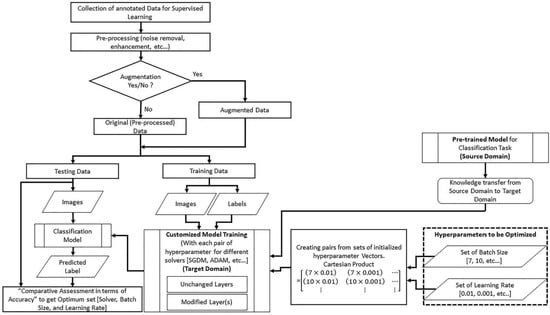
Figure 1. The framework to implement KBTL.

Any pre-trained classification model with its learned parameters can be used after customization. The framework is based on an idea to input hyperparameters in the form of ordered pairs (batch size and learning rate). The ordered pair can be defined as a 2-tuple element of a matrix constructed using the concept of the Cartesian product of two initialized sets of the batch size and learning rate. The following subsections discuss the step-by-step implementation of the transfer learning technique using the adopted framework.

3.1.1. Dataset

Exactly 3064 MR images from a publicly available dataset of 233 patients with brain tumors were used [25]. This collection contained three different types of brain tumor MR images, including 1426 slices of gliomas, 708 slices of meningiomas, and 930 slices of pituitary tumors. Each type of tumor proportion in the dataset is shown in Figure 2 [10]. These data, which are accessible in .mat file (Matlab data format), include a patient ID, a label for the image, the picture as a 512 by 512 matrix, a tumor mask, and discrete point coordinates on the tumor border.

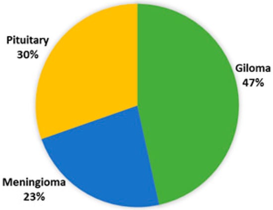
Figure 2. The percentage of different type of tumors in the dataset.

3.1.2. Preprocessing

Data preprocessing, which includes contrast enhancement and normalization, is necessary for medical image analysis. The dataset was first normalized to the intensity values and then mapped to the 256 levels of grayscale using Equation (1):

$$y_{\left(i,j\right)}=\frac{x_{\left(i,j\right)}-x_{min}}{x_{max}-x_{min}}\times 2^8$$

(1)

where $y_{\left(i,j\right)}$ represents any one of the 8-bit grayscale pixel values between 0 and 255 against $x$ at position $\left(i,j\right)$. The variables $x_{max}$ and $x_{min}$ are the maximum and minimum pixel intensity in the original image, respectively. Figure 3 shows the original and enhanced images and Figure 4 presents one sample of each type of tumor.

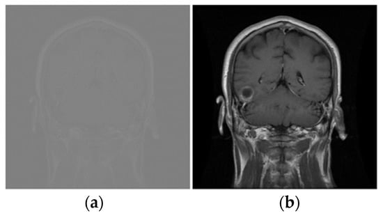
Figure 3. The original and Enhanced Image. (a) Image in dataset; (b) Enhanced Image.

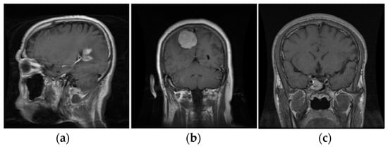
Figure 4. The three types of tumors. (a) Glioma; (b) Meningioma; (c) Pituitary.

The enhanced resultant images were resized and concatenated three times, as per the standard input image size of the pre-trained DL models, to create channels. All three variants of ResNet: ResNet18, ResNet50, and ResNet101, the best-performing pre-trained DL models [10] for brain tumor classification, have a standard input image size of $224\times 224\times 3$.

3.1.3. Pre-Trained DL Models

There were many state-of-the-art pre-trained DL models for the classification task. In this research, the idea behind the adopted framework was domain adaptation, in which transfer learning allowed us to utilize the network and knowledge in terms of network weights of pre-trained DL models, from a source domain, to retrain it using new training data for another classification task in the target domain. The data size and similarity between the target and source domain tasks were important parameters for the pre-trained model selection. Because almost all pre-trained existing DL models are trained on millions of natural images, choosing one pre-trained model directly to implement the transfer learning technique for the classification of brain tumors was quite difficult. We assumed, based on the availability of state-of-the-art pre-trained DL models, that the source domain and target domain were different but the task in both domains was similar i.e., classification task. Since we were extending the scope of the research of [10] through statistical analysis, therefore, for better interpretation, we had to increase the simulated results in terms of accuracy to evaluate and validate the hyperparameter effect individually as well as interactively. For this purpose, in this study we were using only the best-performing models based on ResNet architecture: ResNet18, ResNet50, and ResNet101. Figure 5 shows the network architecture of the ResNet18 model.

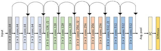
Figure 5. The ResNet18 architecture [26].

The ResNet18 network architecture consists of 18 layers including 17 convolutional layers plus one fully connected layer and an additional softmax layer to perform the classification task. In this study, we used ResNet18 as a network, already trained on ImageNet dataset to classify 1000 objects, for the initialization of weights, and KBTL was performed. KBTL was implemented by replacing the last fully connected (FC) layer with the new FC layer to match the number of classes, which was 3 three for our task. After replacing the layer, the modified network was retrained for our target domain brain tumor multi-classification task. The modified network was trained with different hyperparameter settings, discussed in the next section, and a comparative analysis was performed to find the optimal hyperparameters, ultimately to obtain an optimized model with the highest accuracy. Since ResNet50 and ResNet101 have the same foundation as ResNet18 and both networks are deeper than ResNet18, therefore, we also used these networks to extend our evaluation space and to validate the significance of hyperparameters in the model performance.

3.1.4. Model Training with Hyperparameters

The optimization problem in implementing KBTL, using the classification framework [10], is finding a set of two most important model hyperparameters’ values i.e., the optimal values for the learning rate and batch size that are consistent with knowledge of the used pre-trained model and give the best accuracy for the classification problem. Mathematically, the problem is defined as:

$$f: {ℝ}^n\to ℝ, \mathrm{Find} \left[x_1,x_2\right]=\mathrm{argmin}f\left(x_1,x_2\right), x_1,x_2\in ℝ$$

where $f$ is representing the cost function and $\left(x_1,x_2\right)$ are the two optimal values of learning rate and batch size that help in minimizing the cost function using the solvers: SGDM, Adam, and RMSprop. Mathematically, $f\left(x_1,x_2\right)$ is defined in Equation (2) as the training average cost $f_i\left(x_1,x_2\right)$ with $N$ dataset size.

$$f\left(x_1,x_2\right)=\frac{1}{N}\sum _{i=1}^N{f}_i\left(x_1,x_2\right)$$

(2)

There are three options to compute the gradient updates: utilizing the complete dataset images $N$, using a single image, or a sample of size between 1 and $N$. The three methods are known as batch gradient descent, stochastic gradient descent, and mini-batch gradient descent respectively. The image sample size utilized to update the gradients each time in one iteration is indicated by the hyperparameter batch size $B$.

Networks using SGDM solver [27] can update their weights according to Equation (3):

$$w_{t+1}=w_t-\eta \frac{\partial f}{\partial w_t};$$

(3)

where, $\frac{\partial f}{\partial w_t}={\nabla }_{w}J\left(w_t\right)$ and $\eta$ is representing the learning rate and $w$ are the weights being updated.

The Adam [27] is a relatively straightforward method using first-order gradients that is computationally efficient and has a low memory demand for stochastic optimization. The technique calculates the rate of adaptive learning for each gradient training parameter. For this solver, the weights can be updated using Equation (4):

$$w_t^i=w_{t-1}^i-\frac{\eta }{\sqrt{{\widehat{v}}_t}+ϵ}.{\widehat{m}}_t$$

(4)

where ${\widehat{m}}_t=\frac{m_t}{1-{\beta }_1^t} ; {\widehat{v}}_t=\frac{v_t}{1-{\beta }_2^t} ; m_t={\beta }_1{m}_{t-1}+\left(1-{\beta }_1\right)\frac{\partial f}{\partial w_t} ; v_t={\beta }_2{v}_{t-1}+\left(1-{\beta }_2\right){\left[\frac{\partial f}{\partial w_t}\right]}^2$; $v_t={\beta }_2{v}_{t-1}+\left(1-{\beta }_2\right){\left[\frac{\partial f}{\partial w_t}\right]}^2$; $\frac{\partial f}{\partial w_t}={\nabla }_{w}J\left(w_t\right)$ and $\frac{\partial f}{\partial w_t}={\nabla }_{w}J\left(w_t\right)$ where the value of ${\beta }_1\in \left[0, 1\right]$ indicates how much information from the previous update is required, $m_t$ is the first momentum, which is the running average of the gradients, and $v_t$ is the second momentum, which is the running average of the squared gradients. The first and second momentums after bias correction are ${\widehat{m}}_t$ and ${\widehat{v}}_t$.

The weight updated equation for RMSprop [27] is as follows:

$$w_{t+1}=w_t-\frac{\eta }{\sqrt{E{\left[{\frac{\partial f}{\partial w}}^2\right]}_t+ϵ}}.\frac{\partial f}{\partial w_t}$$

(5)

where, $E{\left[{\frac{\partial f}{\partial w}}^2\right]}_t=0.9E{\left[{\frac{\partial f}{\partial w}}^2\right]}_{t-1}+0.1{\frac{\partial f}{\partial w_t}}^2$. RMSprop divides the learning rate by an average of the squared gradients that decays exponentially. The above equations show that the batch size and learning rate have an impact on each other, and they can have a huge impact on the network performance.

In our previous research work [10], we initialized two different sets $X$ and $Y$ for both hyperparameters, consisting of possible values based on their available values in various studies [46, 50, 53, 62, 68, 69]. We defined $X=\left[7, 10, 32, 128\right]$ and $Y=\left[0.01, 0.001, 0.0001, 0.00001\right]$ for the batch size and learning rate, respectively. A $2-\mathrm{dimensional}$ matrix of size $4\times 4$, containing 2-tuple elements, was generated by taking the Cartesian product of two initialized sets X and Y. The Cartesian product of two sets X and Y is the set of all ordered pairs $\left(x,y\right)$ and can be defined as:

$$X\times Y=\left[\left(x,y\right) | x\in X \mathrm{and} \mathrm{y}\in \mathrm{Y}\right]$$

(6)

It can be generalized to an $n$-ary Cartesian product over $n$ sets $X_1, \dots , X_n$ of different hyperparameters:

$$X_1\times \dots \times X_n=\left[\left(x_1,\dots ,x_n\right) | x_i\in X_i \mathrm{for} \mathrm{every} i\in \left\{1,\dots ,\mathrm{n}\right\}\right]$$

(7)

In our case, we transformed the Cartesian product vector into a matrix for a better understanding, as described in Equation (8):

$$X\times Y=\left[\begin{array}{cccc}\left(7, 0.01\right)& \left(7, 0.001\right)& \left(7, 0.0001\right)& \left(7, 0.00001\right)\\ \left(10, 0.01\right)& \left(10, 0.001\right)& \left(10, 0.0001\right)& \left(10, 0.00001\right)\\ \left(32, 0.01\right)& \left(32, 0.001\right)& \left(32, 0.0001\right)& \left(32, 0.00001\right)\\ \left(128, 0.01\right)& \left(128, 0.001\right)& \left(128, 0.0001\right)& \left(128, 0.00001\right)\end{array}\right]$$

(8)

Each element of the Cartesian product matrix is applied as a pair of inputs for two hyperparameters to retrain the modified network architecture against each pre-trained deep learning model with our dataset for the brain tumor classification task. Each modified network architecture was evaluated for the three most popular solvers: SGDM, ADAM, and RMSProp. An extensive comparative assessment was conducted in terms of accuracy to obtain the optimal values of batch size and learning rate, along with the most appropriate solver.

3.2. Analysis of Variance (ANOVA)

ANOVA is a group of statistical models and their accompanying estimation technique for examining the differences between means. A two-way ANOVA, an extension of ANOVA, is used when data are collected for a quantitative dependent variable (performance) at multiple levels of two independent controlling categorical variables (learning rate and batch size). The categorical variables are called factors and model performances at each row/column factors are known as treatments. ANOVA is based on the total variance law, according to which the variance observed in a given variable is divided into parts attributed to various variation sources [28]. In this study, we used ANOVA to evaluate the significance of the LR and BS factors and their interaction on model performance.

3.2.1. Factor Effects Model

Consider the two categorical variables (factors) $LR$ with levels $i=1,\dots ,a ; BS$ with levels $j=1,\dots ,b$, and $Y_{\left(i,j\right), k}$ representing the $k\mathrm{th}$ treatment observation $\left(k=1,\dots ,r; \mathrm{where} r=a\times b\right)$ at the factor’s level $\left(i,j\right)$. Equation (9) [29] represents the Factor effects model:

$$Y_{\left(i,j\right),k}=\mu +{\theta }_i+{\phi }_j+{\gamma }_{i,j}+{ϵ}_{\left(i,j\right),k}$$

(9)

where, $\mu$ represents the overall mean:

$$\mu ={\mu }_{..}=\frac{{\sum }_{i,j} {\mu }_{i,j}}{ab},$$

(9a)

${\mu }_i$ represents the $i\mathrm{th}$ level of $LR$: ${\mu }_{i.}=\frac{{\sum }_j {\mu }_{i,j}}{b}$,

${\mu }_j$ represents the $j\mathrm{th}$ level of $BS$: ${\mu }_{.j}=\frac{{\sum }_i {\mu }_{i,j}}{a}$

${\theta }_i$ is the main effect due to factor $LR$:

$${\theta }_i={\mu }_{i.}-\mu \Rightarrow {\mu }_{i.}=\mu +{\theta }_i$$

(9b)

${\phi }_j$ is the main effect due to factor $BS$

$${\phi }_j={\mu }_{.j}-\mu \Rightarrow {\mu }_{.j}=\mu +{\phi }_j$$

(9c)

and ${\gamma }_{i,j}$ represents the interaction effect between factors $LR$ and $BS$ and can be defined as:

$$\begin{array}{ll}{\gamma }_{i,j}& ={\mu }_{i,j}-\left(\mu +{\theta }_i+{\phi }_j\right)\\ & ={\mu }_{i,j}-\left(\mu +\left({\mu }_{i.}-\mu \right)+\left({\mu }_{.j}-\mu \right)\right)\\ & ={\mu }_{i,j}-{\mu }_{i.}-{\mu }_{.j}+\mu \end{array}$$

(9d)

These equations also describe the relationship between the factor effects model parameters and cell means ${\mu }_{i,j}$.

3.2.2. Estimates for the Factor Effects Model

Equation (10) represents the overall mean and each group’s means estimation by the overall mean of all treatments/outputs and by the mean of the treatments within that group, respectively.

$$\widehat{\mu }={\overline{Y}}_{\dots }=\frac{{\sum }_{\left(i,j\right),r}{Y}_{\left(i,j\right),k}}{abr}$$

(10)

$${\widehat{\mu }}_{i.}={\overline{Y}}_{i_{..}} \mathrm{and} {\widehat{\mu }}_{.j}={\overline{Y}}_{.j.}$$

(10a)

${\theta }_i$, the main effect due to factor $LR$ can be estimated using Equation (10b):

$${\widehat{\theta }}_i={\overline{Y}}_{i_{..}}-{\overline{Y}}_{\dots }$$

(10b)

${\phi }_i$, the main effect due to factor $BS$ can be estimated using Equation (10c):

$${\widehat{\phi }}_j={\overline{Y}}_{.j.}-{\overline{Y}}_{\dots }$$

(10c)

${\gamma }_{i,j}$, the interaction effect in between factors $LR$ and $BS$ that can be estimated using Equation (10d):

$${\widehat{\gamma }}_{i,j}={\overline{Y}}_{i,j.}-{\overline{Y}}_{i_{..}}-{\overline{Y}}_{.j.}+{\overline{Y}}_{\dots }$$

(10d)

3.2.3. Sum of Squares (SS) for ANOVA Table

SS (total) defines the sum of squares for the overall data, corrected for the overall mean of all accuracies. Equation (11) describes the SS (total), mathematically.

$$\mathrm{SS}\left(total\right)=\mathrm{SS}\left(LR\right)+\mathrm{SS}\left(BS\right)+\mathrm{SS}\left(LR\times BS\right)+\mathrm{SS}\left(E\right)$$

(11)

where,

$$\begin{array}{c}\mathrm{SS}\left(LR\right)=\mathrm{Sum}\mathrm{of}\mathrm{Squares}\mathrm{due}\mathrm{to}\mathrm{factor}LR={\displaystyle \sum }_{\left(i,j\right),r}{\widehat{\theta }}_i{}^2={\displaystyle \sum }_{\left(i,j\right),r}{\left({\overline{Y}}_{i_{..}}-{\overline{Y}}_{\dots }\right)}^2\\ \hfill =rb{\displaystyle \sum }_i{\left({\overline{Y}}_{i_{..}}-\overline{Y}\right)}^2\\ \mathrm{SS}\left(BS\right)=\mathrm{Sum}\mathrm{of}\mathrm{Squares}\mathrm{due}\mathrm{to}\mathrm{factor}BS={\displaystyle \sum }_{\left(i,j\right),r}{\widehat{\phi }}_i{}^2={\displaystyle \sum }_{\left(i,j\right),r}{\left({\overline{Y}}_{.j.}-{\overline{Y}}_{\dots }\right)}^2\\ \hfill =ra{\displaystyle \sum }_j{\left({\overline{Y}}_{.j.}-\overline{Y}\right)}^2\\ \mathrm{SS}\left(LR\times BS\right)=\mathrm{Sum}\mathrm{of}\mathrm{Squares}\mathrm{due}\mathrm{to}\mathrm{interaction}\mathrm{of}\mathrm{factor}LR\&BS={\displaystyle \sum }_{\left(i,j\right),r}{\widehat{\gamma }}_{i,j}^2\\ \hfill =r{\displaystyle \sum }_{\left(i,j\right)}{\widehat{\gamma }}_{i,j}^2\\ \mathrm{SS}\left(E\right)=\mathrm{Error}\mathrm{Sum}\mathrm{of}\mathrm{Squares}={\displaystyle \sum }_{\left(i,j\right),r}{\left(Y_{\left(i,j\right),r}-{\overline{Y}}_{i,j.}\right)}^2={\displaystyle \sum }_{\left(i,j\right),r}{e}_{\left(i,j\right),r}^2\end{array}$$

3.2.4. Degree of Freedom (df) for ANOVA Table

The degree of freedom (df) is the number of independent pieces of information. Mathematically,

$$d{f}_{LR}=\left(a-1\right)$$

(12a)

$$d{f}_{BS}=\left(b-1\right)$$

(12b)

$$d{f}_{LR\times BS}=\left(a-1\right)\left(b-1\right)$$

(12c)

$$d{f}_E=ab\left(r-1\right)$$

(12d)

$$d{f}_{total}=abr-1$$

(12e)

3.2.5. Mean Square (MS) for ANOVA Table

The ratio of the Sum of Squares (SS) and Degree of freedom (df) gives the corresponding Mean Square (MS). Mathematically,

$$MS\left(LR\right)=\mathrm{SS}\left(LR\right)/d{f}_{LR}$$

(13a)

$$MS\left(BS\right)=\mathrm{SS}\left(BS\right)/d{f}_{BS}$$

(13b)

$$MS\left(LR\times BS\right)=\frac{\mathrm{SS}\left(LR\times BS\right)}{d{f}_{LR\times BS}}$$

(13c)

$$MS\left(E\right)=\mathrm{SS}\left(E\right)/d{f}_E$$

(13d)

$$MS\left(total\right)=\mathrm{SS}\left(total\right)/d{f}_{total}$$

(13e)

3.2.6. Hypotheses for Two-Way ANOVA

Test for LR Effect:

Null Hypotheses ${\mathrm{H}}_0: {\theta }_i=0 \mathrm{for} \mathrm{all} i$

Alternate Hypotheses ${\mathrm{H}}_a: {\theta }_i\ne 0 \mathrm{for} \mathrm{at} \mathrm{least} \mathrm{one} i$

The F-statistics for the LR effect test is

$$F_{LR}=\frac{MS\left(LR\right)}{MS\left(E\right)}$$

(14a)

and under the null hypotheses, this follows an F distribution with $d{f}_{LR}, d{f}_E$.

Test for BS Effect:

Null Hypotheses ${\mathrm{H}}_0: {\phi }_j=0 \mathrm{for} \mathrm{all} j$

Alternate Hypotheses ${\mathrm{H}}_a: {\phi }_j\ne 0 \mathrm{for} \mathrm{at} \mathrm{least} \mathrm{one} j$

The F-statistics for the BS effect test is

$$F_{BS}=\frac{MS\left(BS\right)}{MS\left(E\right)}$$

(14b)

and under the null hypotheses, this follows an F distribution with $d{f}_{BS}, d{f}_E$.

Test for LR and BS Interaction Effect:

Null Hypotheses ${\mathrm{H}}_0: {\gamma }_{\left(i,j\right)}=0 \mathrm{for} \mathrm{all} \left(i,j\right)$

Alternate Hypotheses ${\mathrm{H}}_a: {\gamma }_{\left(i,j\right)}\ne 0 \mathrm{for} \mathrm{at} \mathrm{least} \mathrm{one} \left(i,j\right)$

The F-statistics for the LR and BS interaction effect test is

$$F_{LR\times BS}=\frac{MS\left(LR\times BS\right)}{MS\left(E\right)}$$

(14c)

and under the null hypotheses, this follows an F distribution with $d{f}_{LR\times BS}, d{f}_E$.

3.2.7. F-Statistics for the Tests

F-statistics gives p-values, calculated using the F distribution with $\left(d{f}_{\mathrm{Factors}}, d{f}_{\mathrm{Error}}\right)$. A $p\le 0.05$ indicates that the tested effect due to factors LR and BS, either as individuals or with an interaction in between, is statistically significant. Table 1 summarizes all the statistical parameters involved in the statistical analysis.

Table 1. The two-way ANOVA Table, with the individual and interaction effect of LR (column) and BS (rows) [30].

Source	SS	df	MS	F
Columns (LR)	SS (LR)	$\left(a-1\right)$	$MS\left(LR\right)$	$\frac{MS\left(LR\right)}{MS\left(E\right)}$
Rows (BS)	SS (BS)	$\left(b-1\right)$	$MS\left(BS\right)$	$\frac{MS\left(BS\right)}{MS\left(E\right)}$
Interaction (LR × BS)	SS (LR × BS)	$\left(a-1\right)\left(b-1\right)$	$MS\left(LR\times BS\right)$	$\frac{MS\left(LR\times BS\right)}{MS\left(E\right)}$
Error	SS (E)	$ab\left(r-1\right)$	$MS\left(E\right)$
Total	SS (total)	$abr-1$	$MS\left(total\right)$

4. Experimental Setup and Results Analysis

For brain tumor classification, we used the experimental setup based on the methodology described in Section 3, implemented and investigated using a system equipped with NVIDIA GEFORCE GTX 1080—8 GB Graphics and MATLAB 2020. The dataset was divided into 70%, 15%, and 15% for training, validation, and testing of the model, respectively. After customizing all pre-trained deep learning models, experiments were performed with each pair of inputs from the Cartesian product-based matrix of the batch size and learning rate for the three most popular solvers.

To evaluate and validate the impact of both hyperparameters, we increased the number of samples in the specified ranges [10] of the LR and BS to obtain a detailed output distribution for better interpretation. This study used an extended Cartesian product matrix, consisting of 56 two-tuple hyperparameters generated from the following two vectors:

$$\mathrm{LR} ϵ \left[0.01, 0.005, 0.001, 0.0005, 0.0001, 0.00005, 0.00001\right]$$

and

$$\mathrm{BS} ϵ \left[2, 4, 7, 8, 10, 16, 32, 64\right]$$

4.1. Simulated Results

An extensive exercise, comprising 504 simulations on the best-performing [10] three cutting-edge architecture-based pre-trained DL models, ResNet18, ResNet50, and ResNet101 were performed. Additionally, the impact was also assessed by using three well-known optimization algorithms (solvers): the adaptive moment estimation (Adam), the stochastic gradient descent with momentum (SGDM), and the root mean squared propagation (RMSProp). The three best-performing ResNet variants were selected with the help of a comparative analysis in which three ResNet variants were compared with other start-of-the-art classification models as presented in Table 2. The parameters to compare were the number of epochs utilized in convergence, number of iterations, validation accuracy, training time, and confusion matrix. All three variants of ResNet, especially ResNet18, outperformed all other networks with parameters {SGDM, 32, 0.01} by achieving 99.56% accuracy when using our framework for brain tumor classification. This was due to the ResNet working principle of building a deeper network compared to other networks and its capability to solve the vanishing gradient problem simultaneously. Figure 6a,b depict the training-validation accuracy and loss curve and the confusion matrix while training, validating, and testing ResNet18, the best-performing model. In addition to the ultimate accuracy measurement, utilizing three other measures: precision, recall, and specificity, the framework was further evaluated. Table 3 summarizes the performance measures related to the above-mentioned measuring parameters for the average of all classes and each class separately as well for all deep learning networks presented in Table 2. The comparison shows that ResNet18 outperforms all the others in all the measuring fields. Figure 6 clearly describes the condition that we had achieved a solution of our optimization problem, defined in Section 3.1.4, with the optimal hyperparameters’ values ($x_1=\mathrm{LR}=0.01 \mathrm{and} x_2=\mathrm{BS}=32$) using the SGDM solver. The solution, ultimately, provided us with an optimized model with the highest accuracy of 99.56% for the brain tumor classification problem.

Table 2. A comparative study of the models with their optimal parameters [10].

Pre-Trained Model	Confusion Matrix	Predicted Class				Solver	Batch Size	Learning Rate	Epoch	Validation Accuracy (%)	Testing Accuracy (%)	Training Time
		G		M	P
AlexNet	True Class	G	210	3	1	SGDM	32	0.001	54	97.17	97.6	0:14:44
		M	2	101	3
		P	0	2	137
GoogleNet (ImageNet)	True Class	G	210	4	0	Adam	10	0.0001	16	98.4	97.39	00:16:03
		M	2	101	3
		P	1	2	136
GoogleNet (Places365)	True Class	G	210	4	0	SGDM	10	0.001	20	98.26	97.17	00:14:42
		M	6	99	1
		P	1	1	137
ResNet-50	True Class	G	213	1	0	SGDM	7	0.001	17	98.26	99.56	0:24:46
		M	1	105	0
		P	0	0	139
ResNet-101	True Class	G	213	1	0	SGDM	10	0.001	23	98.26	99.35	0:51:04
		M	1	105	0
		P	1	0	138
ResNet-18	True Class	G	213	1	0	SGDM	32	0.01	54	98.48	99.56	0:19:25
		M	0	105	1
		P	0	0	139
VGG16	True Class	G	214	0	0	SGDM	7	0.0001	11	96.74	98.26	0:14:41
		M	6	98	2
		P	0	0	139
VGG19	True Class	G	211	3	0	SGDM	7	0.0001	15	97.17	98.69	0:21:24
		M	1	105	0
		P	0	2	137
SqueezeNet	True Class	G	208	5	1	SGDM	32	0.001	36	97.39	97.39	0:11:18
		M	1	103	2
		P	2	1	136
MobileNet	True Class	G	213	1	0	SGDM	32	0.01	54	97.61	98.91	0:43:46
		M	1	103	2
		P	0	1	138
Inception V3	True Class	G	211	3	0	RMS-Prop	10	0.0001	20	98.04	98.26	0:58:39
		M	1	103	2
		P	1	1	137

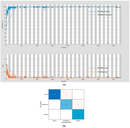
Figure 6. (a) The training-validation accuracy and loss for the best-performing model. (b) The confusion matrix for the best-performing model.

Table 3. A comparative study of the models in terms of performance metrics [10].

Fine-Tune Models	Precision Per Class	Average Precision	Sensitivity Per Class	Average Sensitivity	Specificity Per Class	Average Specificity
AlexNet	99.06%	97.61%	98.13%	97.60%	99.18%	98.91%
	95.28%		95.28%		98.58%
	97.16%		98.56%		98.75%
GoogleNet (ImageNet)	98.11%	96.97%	97.20%	96.95%	98.37%	98.53%
	92.59%		94.34%		97.73%
	98.56%		98.56%		99.38%
GoogleNet (Places365)	96.77%	97.17%	98.13%	97.17%	97.14%	98.25%
	95.19%		93.40%		98.58%
	99.28%		98.56%		99.69%
ResNet50	99.53%	99.56%	99.53%	99.56%	99.59%	99.74%
	99.06%		99.06%		99.72%
	100.00%		100.00%		100.00%
ResNet101	99.07%	99.35%	99.53%	99.35%	99.18%	99.55%
	99.06%		99.06%		99.72%
	100.00%		99.28%		100.00%
ResNet18	100.00%	99.57%	99.53%	99.56%	100.00%	99.84%
	99.06%		99.06%		99.72%
	99.29%		100.00%		99.69%
VGG16	97.27%	98.30%	100.00%	98.26%	97.55%	98.67%
	100.00%		92.45%		100.00%
	98.58%		100.00%		99.38%
VGG19	99.53%	98.73%	98.60%	98.69%	99.59%	99.48%
	95.45%		99.06%		98.58%
	100.00%		98.56%		100.00%
SqueezeNet	98.58%	97.41%	97.20%	97.39%	98.78%	98.75%
	94.50%		97.17%		98.30%
	97.84%		97.84%		99.06%
MobileNet	99.53%	98.91%	99.53%	98.91%	99.59%	99.49%
	98.10%		97.17%		99.43%
	98.57%		99.28%		99.38%
InceptionV3	99.06%	98.26%	98.60%	98.26%	99.18%	99.17%
	96.26%		97.17%		98.87%
	98.56%		98.56%		99.38%

In this study, as discussed above, we extended the scope of the research by performing a statistical analysis to evaluate and validate the effect of the hyperparameters. All three models with three different solvers were simulated with each pair (LR, and BS) from the extended Cartesian product matrix for 100 epochs. Seven LRs and eight BSs in the form of pairs resulted in 56 test accuracies with one solver for one model. Table 4 presents all three models’ performances in terms of accuracies for the three solvers.

Table 4. ResNet architecture-based models’ performances in term of accuracies (percentage).

		ResNet18							ResNet50							ResNet101
		SGDM							SGDM							SGDM
	LR	0.01	0.005	0.001	5 × 10−4	1 × 10−4	5 × 10−5	1 × 10−5	0.01	0.005	0.001	5 × 10−4	1 × 10−4	5 × 10−5	1 × 10−5	0.01	0.005	0.001	5 × 10−4	1 × 10−4	5 × 10−5	1 × 10−5
BS
2		93.03	94.55	97.17	98.91	95.21	95.86	88.02	92.59	94.99	96.95	98.26	95.86	96.73	92.16	78.87	94.77	96.08	97.6	95.64	94.77	89.76
4		95.21	96.51	97.39	98.04	94.55	96.73	90.2	96.95	94.99	98.04	98.69	96.08	96.73	94.12	97.6	97.82	97.82	97.6	95.42	94.12	93.9
7		95.64	93.25	98.91	98.26	97.82	95.21	95.86	96.73	98.04	99.56	97.82	97.17	97.17	95.21	98.69	98.04	97.82	98.26	97.17	95.42	95.86
8		95.64	97.17	97.6	96.95	96.08	93.25	93.68	97.17	96.73	98.26	97.82	95.64	95.86	95.64	97.6	98.91	98.69	97.39	96.3	95.21	93.03
10		97.82	96.3	98.91	96.73	96.73	94.12	95.42	97.6	98.26	99.35	97.17	96.95	96.08	96.3	98.04	97.17	99.35	98.91	96.73	95.42	94.34
16		96.08	97.82	96.73	97.39	94.99	95.86	91.5	98.69	98.04	98.04	96.95	95.42	97.17	91.94	98.04	98.69	98.04	97.82	96.08	95.64	93.25
32		99.56	98.47	96.3	95.21	97.39	94.77	94.34	97.39	96.73	97.82	96.95	95.86	94.99	92.37	98.69	98.47	95.64	96.3	95.21	94.12	93.9
64		97.39	96.3	96.51	94.99	93.9	93.03	89.32	97.17	96.51	94.77	96.3	95.42	96.3	89.54	97.6	98.04	95.17	95.82	95.04	92.37	92.16
		ADAM							ADAM							ADAM
2		66.23	89.54	92.59	95.86	97.39	95.86	97.39	68.63	76.47	90.58	96.51	97.82	96.95	95.86	62.96	79.08	65.58	90.41	97.17	94.99	91.29
4		76.03	87.36	93.03	95.21	98.91	96.08	95.86	69.72	88.89	93.9	92.16	96.51	95.42	96.95	71.68	86.06	93.9	89.76	97.39	97.82	98.26
7		91.29	93.68	93.9	95.21	98.47	95.42	96.3	80.61	83.22	96.08	97.39	98.26	98.47	94.99	79.74	88.24	92.37	96.95	97.39	97.39	96.73
8		84.75	91.72	96.08	96.95	98.47	95.64	96.08	78.43	94.55	94.55	91.29	97.82	98.91	96.73	84.1	84.97	93.25	97.6	99.13	97.17	95.64
10		81.48	94.34	92.81	98.26	98.04	95.42	96.3	90.41	94.55	95.64	95.21	98.26	97.39	95.42	88.45	92.81	92.59	95.86	97.17	97.6	96.73
16		94.77	91.29	96.08	98.47	97.6	99.13	96.08	91.72	92.59	95.21	97.17	99.13	98.91	96.3	83.01	90.2	94.77	97.17	98.47	96.3	94.34
32		94.12	94.99	96.95	98.47	98.91	98.69	95.21	87.58	95.21	96.51	98.04	97.17	98.91	96.08	93.46	91.7	91.29	96.51	97.82	97.6	95.64
64		96.51	95.86	96.3	96.08	98.91	98.04	97.39	92.16	95.86	95.21	95.64	98.26	98.91	93.9	90.63	90.81	91.7	95.21	97.39	96.51	93.04
		RMSProp							RMSProp							RMSProp
2		76.25	80.39	84.31	89.54	95.64	97.39	96.95	64.71	81.92	85.4	83.88	98.26	96.51	96.95	23.09	64.92	82.79	79.96	96.73	98.04	94.12
4		76.03	82.79	92.16	93.25	98.69	97.39	95.42	78.65	87.15	92.16	93.25	98.47	97.82	98.04	78.43	84.53	89.32	94.12	98.04	98.91	95.64
7		90.63	92.81	91.29	93.25	95.64	97.39	96.95	76.47	88.24	88.45	97.82	98.91	97.17	95.42	79.3	81.05	90.41	95.42	96.51	98.04	96.08
8		93.68	89.54	95.42	94.99	98.26	98.69	97.6	85.84	82.35	91.5	96.95	98.04	97.6	98.26	86.71	87.58	91.72	94.55	98.04	98.47	95.64
10		86.06	90.63	94.55	90.63	97.6	98.26	96.3	86.93	89.98	92.75	94.99	96.73	98.69	96.73	89.11	91.5	94.34	94.34	98.47	97.6	97.6
16		87.58	92.81	96.51	96.51	98.47	98.04	97.6	83.22	89.54	93.03	97.39	97.17	98.47	95.86	83.66	91.29	93.9	93.03	96.3	97.82	96.73
32		90.2	90.85	94.55	95.64	97.39	97.17	96.51	88.89	91.94	94.77	91.07	97.82	98.91	96.51	85.19	90.72	97.17	95.64	97.82	98.04	96.8
64		91.07	93.68	74.73	94.77	98.04	96.51	95.64	91.5	89.98	95.86	96.51	97.39	98.26	94.77	80.61	88.89	94.55	93.9	95.21	97.39	95.86

Furthermore, Figure 7 shows boxplots, demonstrating the collected results’ distribution for the ResNet18 DL model retrained on our brain tumor dataset with solvers SGDM, Adam, and RMSProp. On the left side, each boxplot exhibits a distribution of measured accuracies for the given range of BSs at each specific LR starting from 0.00001 to 0.01. On the right side, each boxplot exhibits a distribution of the measured accuracies for the given range of LRs at each specific BS starting from 2 to 64. Each boxplot represents the lower quartile, median, and upper quartile, and whiskers extend to the end of the sample range to display the maximum and minimum accuracies.

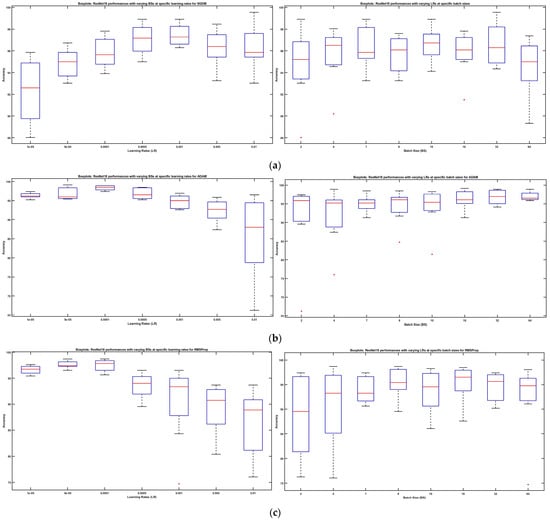
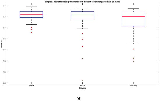
Figure 7. (a) ResNet18 performances with SGDM: varying BSs at specific LRs (left side), varying LRs at specific BSs (right side). (b) ResNet18 performances with ADAM: varying BSs at specific LRs (left side), varying LRs at specific BSs (right side). (c) ResNet18 performances with RMSProp: varying BSs at specific LRs (left side), varying LRs at specific BSs (right side). (d) ResNet18 model performances with three solvers for paired hyperparameter inputs.

On increasing the LRs, the parameters of the boxplots display a nonlinear behavior. When referring to SGDM, the maximum accuracy of 99.56% i.e., the highest value of the whiskers, was observed with LR = 0.01 while the maximum dispersion was observed with the lowest value of LR = 0.00001. On the other hand, with Adam, the maximum value of the whiskers (accuracy = 99.13%) was observed with LR = 0.00005, whereas the greatest dispersion was depicted with LR = 0.01. RMSProp informed of a behavior similar to Adam, with the greatest dispersion being at the highest value of LR and the maximum performance being at LR = 0.00005. Similarly, on the right side of Figure 7, boxplots about the increase in the batch size reveal a nonlinear pattern. Conclusively, it is quite evident from the boxplots that increasing/decreasing the LRs and BS did not increase/decrease the model performance in a hierarchical fashion, rather there seemed to be a trade-off in-between.

Figure 7d reveals the joint impact of LR and BS on the data set while comparing the model performances using SGDM, Adam, and RMSProp. We observed that concerning the brain tumor classification, SGDM had the most optimum performance in comparison to Adam and RMSProp as it reached the maximum accuracy and has the lowest dispersion too. The dispersion of outputs was gradually increasing in Adam and RMSProp, respectively. Although the whiskers maxima and the upper quartile were almost the same for all three solvers, the lower quartile was gradually decreasing. Conclusively, the experimental results show that both hyperparameters (LR and BS) had a significant impact individually as well as interactively, with a trade-off in between.

Similar experiments were performed for ResNet50, and ResNet101 models to collect the relevant data in terms of accuracies for the defined values of LR and BS. Simulation results revealed the same effect of LR and BS on the model performance as shown by ResNet18.

A performance comparison is presented in Table 5 between our work and other existing state-of-the-art research studies that used the same brain tumor dataset for multi-type tumor classification. The comparison was mainly based on the performance metric “accuracy” with the support of three other parameters: “precision,” “recall,” and “specificity.” The comparison showed that the transfer learning technique, implemented through our proposed framework for brain tumor classification, outperformed all existing approaches based on traditional image processing [5,31], CNN [32,33], and transfer learning [34,35,36,37,38,39,40].

Table 5. The comparison of the framework with the related work based on the same dataset.

Related Work	Approach	Accuracy	Precision				Recall				Specificity
			G	M	P	Average	G	M	P	Average	G	M	P	Average
[5]	BoW-SVM	91.28	-	-	-	-	96.4	86	87.3	-	96.3	95.5	95.3	-
[31]	DWT-Gabor-NN	91.90	-	-	-	-	95.1	86.9	91.2	-	96.3	96	95.7	-
[32]	CapsNet	90.89	-	-	-	-	-	-	-	-	-	-	-	-
[33]	CNN-ELM	93.68	91	94.5	98.3	-	97.5	76.8	100	-	-	-	-	-
[34]	VGG19	94.58	-	-	-	-	-	-	-	88.41	-	-	-	96.12
[35]	VGG19	94.82	93	87.97	87.34	89.52	95.97	89.98	96.81	94.25	93.79	96.42	93.93	94.69
[36]	GoogleNet-SVM	97.10	99	94.7	98	-	97.9	96	98.9	-	99.4	98.4	99.1	-
[40]	VGG16	98.69	-	-	-	-	-	-	-	-	-	-	-	-
[37]	VGGNet	94.00	-	-	-	-	-	-	-	-	-	-	-	-
[38]	DenseNet	99.51	99	99	100	-	100	99	99	-	-	-	-	-
[39]	GoogleNet-KNN	98.30	98	95.55	97.78	-	98.02	94.57	99.1	-	98.63	98.65	99.01	-
Our Approach	ResNet18	99.56	100	99.06	99.29	99.45	99.53	99.06	100	99.53	100	99.72	99.69	99.8

4.2. Statistical Analysis

The discussion in this section validates our experimental results using two-way ANOVA. The analysis was performed using the collected data in terms of test accuracies, shown in Table 4 as well as in Figure 7 boxplots. Each accuracy represented an output against each pair of LR and BS for the ResNet18 model with solvers SGDM, Adam, and RMSProp. The statistical analysis has validated our experimental findings: (1) LR showed a significant impact on the model performance, (2) BS showed a significant impact on the model performance, and (3) there was an interaction effect of LR and BS on the model performance.

In addition to the representation of data as boxplots, a sample of data to describe how it was used in the analysis is shown in Table 6.

Table 6. The dataset sample (the ResNet model’s performances (accuracies) with SGDM) organized for ANOVA statistics [30].

LR BS	0.01	0.005	0.001	0.0005	0.0001	0.00005	0.00001
2	93.03	94.55	97.17	98.91	95.21	95.86	88.02
	92.59	94.99	96.95	98.26	95.86	96.73	92.16
	78.87	94.77	96.08	97.60	95.64	94.77	89.76
4	95.21	96.51	97.39	98.04	94.55	96.73	90.20
	96.95	94.99	98.04	98.69	96.08	96.73	94.12
	97.60	97.82	97.82	97.60	95.42	94.12	93.90

The columns of the matrix represent the LRs and the rows represent the BSs. In this analysis, we replicated each experiment three times, as per the ANOVA statistics, for a balanced design. The first three rows correspond to ResNet18, ResNet50, and ResNet101, respectively for BS = 2 and the next three rows represent the performances for all three models with BS = 4. The response values are the model performances in terms of accuracy at each (LR, BS) paired value.

Table 7 shows the parameters obtained through the ANOVA analysis. The parameter $\mathrm{Prob}>\mathrm{F}$ shows the p-values: $3.52524\times {10}^{-20}, 2.4884\times {10}^{-09}, \mathrm{and} 6.57531\times {10}^{-07}$ for the LRs, BSs, and the interaction effect between LR and BS, respectively. These values indicate that LRs and BSs affected the model performance individually as well as there was an interaction between the two hyperparameters. Further, we have also performed multiple comparison tests to investigate whether the model performance differed between pairs of LRs or not. The test helped us in finding the significant impact on the model performance due to an increase/decrease in the LR.

Table 7. The two-way ANOVA, individual and interaction effect of LR (column) and BS (rows).

Source	SS	df	MS	F	Prob > F
LRs	367.89	6	61.3145	27.91	3.52524 × 10−20
BSs	148.04	7	21.148	9.63	2.4884 × 10−9
Interaction	292.94	42	6.9748	3.17	6.57531 × 10−7
Error	246.07	112	2.1971
Total	1054.94	167

Table 8 shows the multiple comparisons of the means of accuracies associated with each LR. Seven LRs are representing seven groups to compare.

Table 8. The two-way ANOVA, multiple comparisons of LR’s (column-wise) means.

Group A	Group B	Lower Limit	A-B	Upper Limit	p-Value
1	2	−1.9294	−0.64458	0.6402	0.74045
1	3	−2.5744	−1.2896	−0.0047974	0.048506
1	4	−2.4115	−1.1267	0.15812	0.12605
1	5	−1.0219	0.26292	1.5477	0.99624
1	6	−0.44145	0.84333	2.1281	0.43887
1	7	2.1056	3.3904	4.6752	3.71 × 10−8
2	3	−1.9298	−0.645	0.63979	0.73987
2	4	−1.7669	−0.48208	0.8027	0.9186
2	5	−0.37729	0.9075	2.1923	0.34781
2	6	0.20313	1.4879	2.7727	0.01243
2	7	2.7502	4.035	5.3198	3.71 × 10−8
3	4	−1.1219	0.16292	1.4477	0.99975
3	5	0.26771	1.5525	2.8373	0.0076499
3	6	0.84813	2.1329	3.4177	4.61 × 10−5
3	7	3.3952	4.68	5.9648	3.71 × 10−8
4	5	0.1048	1.3896	2.6744	0.025044
4	6	0.68521	1.97	3.2548	0.00021833
4	7	3.2323	4.5171	5.8019	3.71 × 10−8
5	6	−0.70437	0.58042	1.8652	0.82336
5	7	1.8427	3.1275	4.4123	3.79 × 10−8
6	7	1.2623	2.5471	3.8319	6.74 × 10−7

Column 1 and column 2 of Table 3 show the LR’s associated groups that are compared. Column number 4 shows the difference between the calculated group means. Column numbers 3 and 5 represent the lower and upper limits, respectively, for the 95% confidence interval for the true mean difference. The last column consists of the p-value for a hypothesis testing that the difference between the corresponding group means is equal to zero. It is very clear from Table 4 that the larger group mean difference resulted in a p-value < 0.05. The p-values in Table 4 that are very small, indicate that the model performance varied across LRs. Conclusively, the LR had a significant impact on the model performance.

Similarly, another multiple comparison was performed to investigate the impact of BS on the model performance. Table 9 shows the multiple comparisons of the means of accuracies associated with each BS. There are eight accuracies groups associated with eight BSs. The small p-values < 0.05 indicate that the model performance differed between two BSs and the group means were significantly different from each other. It is concluded that BS had a significant impact on the model performance.

Table 9. Two-way ANOVA, multiple comparisons of BS’s (row-wise) means.

Group A	Group B	Lower Limit	A-B	Upper Limit	p-Value
1	2	−3.3525	−1.9395	−0.5265	0.0012
1	3	−4.2764	−2.8633	−1.4503	2.6014 × 10−7
1	4	−3.6435	−2.2305	−0.8175	9.5937 × 10−5
1	5	−4.2664	−2.8533	−1.4403	2.8206 × 10−7
1	6	−3.6225	−2.2095	−0.7965	1.1579 × 10−4
1	7	−3.4464	−2.0333	−0.6203	5.3643 × 10−4
1	8	−2.1325	−0.7195	0.6935	0.7653
2	3	−2.3368	−0.9238	0.4892	0.4736
2	4	−1.7040	−0.2910	1.1221	0.9983
2	5	−2.3268	−0.9138	0.4992	0.4881
2	6	−1.6830	−0.2700	1.1430	0.9989
2	7	−1.5068	−0.0938	1.3192	1.0000
2	8	−0.1930	1.2200	2.6330	0.1439
3	4	−0.7802	0.6329	2.0459	0.8629
3	5	−1.4030	0.0100	1.4230	1.0000
3	6	−0.7592	0.6538	2.0668	0.8418
3	7	−0.5830	0.8300	2.2430	0.6117
3	8	0.7308	2.1438	3.5568	2.0727 × 10−4
4	5	−2.0359	−0.6229	0.7902	0.8724
4	6	−1.3921	0.0210	1.4340	1.0000
4	7	−1.2159	0.1971	1.6102	0.9999
4	8	0.0979	1.5110	2.9240	0.0272
5	6	−0.7692	0.6438	2.0568	0.8521
5	7	−0.5930	0.8200	2.2330	0.6264
5	8	0.7208	2.1338	3.5468	2.2624 × 10−4
6	7	−1.2368	0.1762	1.5892	0.9999
6	8	0.0770	1.4900	2.9030	0.0311
7	8	−0.0992	1.3138	2.7268	0.0883

Kandel et al. [20] used five different BS(s) and two LR(s) to investigate these hyperparameters’ influence on the network’s performance. The author concluded that the performance was significantly influenced by the learning rate and batch size; the learning rate and batch size had a high correlation. The author advised choosing small batch sizes with a low learning rate. According to a Masters et al. [22] statement, small BS(s) should be used. The author did not comment on the influence of LR while Radiuk [19] said that a higher BS should be used with a large LR to obtain a better performance. All these research studies used very limited experiments with few LR(s) and BS(s) that could not guarantee the exact pattern. In our case, we performed an extensive exercise with a larger number of LR(s) and BS(s) to find the pattern. From our simulation results, presented in Table 4, it is quite clear that both hyperparameters have a significant influence on the model performance with a trade-off in-between. Further, the ANOVA statistical test also proved that both hyperparameters not only have an individual significant effect on the model performance but also an interaction exists in-between.

5. Conclusions and Future Work

The successful implementation of KBTL is completely based on the tuning of hyperparameters such as the LR and BS. In addition to the challenging task of selecting an optimal value for hyperparameters, there is another issue to find their significant impact, independently as well as interactively, on the model performance. In this study, a Cartesian product matrix, consisting of 56 pairs of LR and BS, was used to input the three best-performing ResNet architecture-based DL models for brain tumor classification. In the first phase, an extensive experiment comprising 504 simulations was performed, and results in terms of the accuracy were collected for further investigation. The initial study revealed that increasing/decreasing the LRs and BS did not increase/decrease the model performance in a hierarchical fashion, rather there seemed to be a trade-off in-between. Further, the experimental results showed that both hyperparameters (LR and BS) had a joint significant impact on the model performance. In the second phase, the results were validated using the statistical ANOVA analysis. The F-test returned all three results, with $p<0.05$, stating both hyperparameters (LR and BS) not only have a significant impact on the model performance independently, but there exists an interaction between LR and BS for a combination of their levels. In addition to these findings, multiple comparison tests for different LRs and different BSs concluded that each LR and BS had an independent impact on the model performance. Further, the non-linear pattern for accuracy on increasing/decreasing LR and BS suggested that there should be a trade-off between LR and BS to obtain the maximum accuracy, ultimately helping to find the optimal values of LR and BS and the optimum model for brain tumor classification.

This study can be further extended by using more than two hyperparameters in the Cartesian product matrix to obtain their optimal values. Moreover, researchers are invited to further validate the methodology by using other dataset(s) for not only brain tumor classification but also in other classification problems. The limitation of this research was the GPU specifications that allowed for the evaluation and validation of the framework for the batch sizes up to 64.

References

- Selvanayaki, K.; Karnan, M. CAD system for automatic detection of brain tumor through magnetic resonance image-a review. Int. J. Eng. Sci. Technol. 2010, 2, 2. [Google Scholar]
- Brindle, K.M.; Izquierdo-García, J.L.; Lewis, D.Y.; Mair, R.J.; Wright, A.J. Brain Tumor Imaging. J. Clin. Oncol. 2017, 35, 2432–2438. [Google Scholar] [CrossRef] [PubMed]
- Wen, P.Y.; Macdonald, D.R.; Reardon, D.A.; Cloughesy, T.F.; Sorensen, A.G.; Galanis, E.; DeGroot, J.; Wick, W.; Gilbert, M.R.; Lassman, A.B.; et al. Updated Response Assessment Criteria for High-Grade Gliomas: Response Assessment in Neuro-Oncology Working Group. J. Clin. Oncol. 2010, 28, 1963–1972. [Google Scholar] [CrossRef]
- Drevelegas, A. Imaging of Brain Tumors with Histological Correlations; Springer: Berlin/Heidelberg, Germany, 2011; pp. 13–33. [Google Scholar]
- Cheng, J.; Huang, W.; Cao, S.; Yang, R.; Yang, W.; Yun, Z.; Wang, Z.; Feng, Q. Enhanced performance of brain tumor classification via tumor region augmentation and partition. PloS ONE 2015, 10, e0140381. [Google Scholar] [CrossRef] [PubMed]
- Cheng, J.; Yang, W.; Huang, M.; Huang, W.; Jiang, J.; Zhou, Y.; Yang, R.; Zhao, J.; Feng, Y.; Feng, Q.; et al. Retrieval of Brain Tumors by Adaptive Spatial Pooling and Fisher Vector Representation. PLoS ONE 2016, 11, e0157112. [Google Scholar] [CrossRef]
- Kumar, S.; Dabas, C.; Godara, S. Classification of Brain MRI Tumor Images: A Hybrid Approach. Procedia Comput. Sci. 2017, 122, 510–517. [Google Scholar] [CrossRef]
- Mohan, G.; Subashini, M.M. MRI based medical image analysis: Survey on brain tumor grade classification. Biomed. Signal Process. Control 2018, 39, 139–161. [Google Scholar] [CrossRef]
- Yang, F.; Zhang, W.; Tao, L.; Ma, J. Transfer Learning Strategies for Deep Learning-based PHM Algorithms. Appl. Sci. 2020, 10, 2361. [Google Scholar] [CrossRef]
- Usmani, I.A.; Qadri, M.T.; Zia, R.; Aziz, A.; Saeed, F. Cartesian Product Based Transfer Learning Implementation for Brain Tumor Classification. Comput. Mater. Contin. 2022, 73, 4369–4392. [Google Scholar] [CrossRef]
- Bahmani, M.; Shawi, R.E.; Potikyan, N.; Sakr, S. To tune or not to tune? An Approach for Recommending Important Hyperparameters. arXiv 2021, arXiv:2108.13066. [Google Scholar]
- He, K.; Zhang, X.; Ren, S.; Sun, J. Deep residual learning for image recognition. In Proceedings of the IEEE Conference on Computer Vision and Pattern Recognition, Las Vegas, NV, USA, 26 June–1 July 2016; pp. 770–778. [Google Scholar]
- Krizhevsky, A.; Sutskever, I.; Hinton, G.E. Imagenet classification with deep convolutional neural networks. Commun. ACM 2017, 60, 84–90. [Google Scholar] [CrossRef]
- Szegedy, C.; Liu, W.; Jia, Y.; Sermanet, P.; Reed, S.; Anguelov, D.; Erhan, D.; Vanhoucke, V.; Rabinovich, A. Going deeper with convolutions. In Proceedings of the IEEE Conference on Computer Vision and Pattern Recognition, Boston, MA, USA, 7–12 June 2015; pp. 1–9. [Google Scholar]
- Simonyan, K.; Zisserman, A. Very deep convolutional networks for large-scale image recognition. arXiv 2014, arXiv:1409.1556. [Google Scholar]
- Iandola, F.N.; Han, S.; Moskewicz, M.W.; Ashraf, K.; Dally, W.J.; Keutzer, K. SqueezeNet: AlexNet-level accuracy with 50x fewer parameters and <0.5 MB model size. arXiv 2016, arXiv:1602.07360. [Google Scholar]
- Sandler, M.; Howard, A.; Zhu, M.; Zhmoginov, A.; Chen, L.-C. Mobilenetv2: Inverted residuals and linear bottlenecks. In Proceedings of the IEEE Conference on Computer Vision and Pattern Recognition, Salt Lake City, UT, USA, 18–23 June 2018; pp. 4510–4520. [Google Scholar]
- Szegedy, C.; Vanhoucke, V.; Ioffe, S.; Shlens, J.; Wojna, Z. Rethinking the inception architecture for computer vision. In Proceedings of the IEEE Conference on Computer Vision and Pattern Recognition, Las Vegas, NV, USA, 27–30 June 2016; pp. 2818–2826. [Google Scholar]
- Radiuk, P.M. Impact of Training Set Batch Size on the Performance of Convolutional Neural Networks for Diverse Datasets. Inf. Technol. Manag. Sci. 2017, 20, 20–24. [Google Scholar] [CrossRef]
- Kandel, I.; Castelli, M. The effect of batch size on the generalizability of the convolutional neural networks on a histopathology dataset. ICT Express 2020, 6, 312–315. [Google Scholar] [CrossRef]
- Bengio, Y. Practical Recommendations for Gradient-Based Training of Deep Architectures. In Neural Networks: Tricks of the Trade; Springer: Berlin/Heidelberg, Germany, 2012; pp. 437–478. [Google Scholar]
- Masters, D.; Luschi, C. Revisiting small batch training for deep neural networks. arXiv 2018, arXiv:1804.07612. [Google Scholar]
- Russakovsky, O.; Deng, J.; Su, H.; Krause, J.; Satheesh, S.; Ma, S.; Huang, Z.; Karpathy, A.; Khosla, A.; Bernstein, M. Imagenet large scale visual recognition challenge. Int. J. Comput. Vis. 2015, 115, 211–252. [Google Scholar] [CrossRef]
- Krizhevsky, A.; Hinton, G. Learning Multiple Layers of Features from Tiny Images. 2009. Available online: http://www.cs.utoronto.ca/~kriz/learning-features-2009-TR.pdf (accessed on 7 January 2023).
- Cheng, J. Brain Tumor Dataset, Version 5. 2017. Available online: https://doi.org/10.6084/m9.figshare.1512427.v5 (accessed on 2 April 2017).
- Ramzan, F.; Khan, M.U.G.; Rehmat, A.; Iqbal, S.; Saba, T.; Rehman, A.; Mehmood, Z. A Deep Learning Approach for Automated Diagnosis and Multi-Class Classification of Alzheimer’s Disease Stages Using Resting-State fMRI and Residual Neural Networks. J. Med. Syst. 2019, 44, 37. [Google Scholar] [CrossRef]
- Yaqub, M.; Feng, J.; Zia, M.; Arshid, K.; Jia, K.; Rehman, Z.; Mehmood, A. State-of-the-Art CNN Optimizer for Brain Tumor Segmentation in Magnetic Resonance Images. Brain Sci. 2020, 10, 427. [Google Scholar] [CrossRef]
- Wu, S.; Hu, X.; Zheng, W.; He, C.; Zhang, G.; Zhang, H.; Wang, X. Effects of reservoir water level fluctuations and rainfall on a landslide by two-way ANOVA and K-means clustering. Bull. Eng. Geol. Environ. 2021, 80, 5405–5421. [Google Scholar] [CrossRef]
- Rouder, J.N.; Schnuerch, M.; Haaf, J.M.; Morey, R.D. Principles of Model Specification in ANOVA Designs. Comput. Brain Behav. 2022, 1–14. [Google Scholar] [CrossRef]
- Mahajan, R.; Kishore, K.; Jaswal, V. The challenges of interpreting ANOVA by dermatologists. Indian Dermatol. Online J. 2022, 13, 109. [Google Scholar] [CrossRef] [PubMed]
- Ismael, M.R.; Abdel-Qader, I. Brain tumor classification via statistical features and back-propagation neural network. In Proceedings of the 2018 IEEE International Conference on Electro/Information Technology (EIT), Rochester, MI, USA, 3–5 May 2018; pp. 0252–0257. [Google Scholar]
- Afshar, P.; Mohammadi, A.; Plataniotis, K.N. Brain tumor type classification via capsule networks. In Proceedings of the 2018 25th IEEE International Conference on Image Processing (ICIP), Athens, Greece, 7–10 October 2018; pp. 3129–3133. [Google Scholar]
- Pashaei, A.; Sajedi, H.; Jazayeri, N. Brain tumor classification via convolutional neural network and extreme learning machines. In Proceedings of the 2018 8th International Conference on Computer and Knowledge Engineering (ICCKE), Mashhad, Iran, 25–26 October 2018; pp. 314–319. [Google Scholar]
- Sajjad, M.; Khan, S.; Muhammad, K.; Wu, W.; Ullah, A.; Baik, S.W. Multi-grade brain tumor classification using deep CNN with extensive data augmentation. J. Comput. Sci. 2018, 30, 174–182. [Google Scholar] [CrossRef]
- Swati, Z.N.K.; Zhao, Q.; Kabir, M.; Ali, F.; Ali, Z.; Ahmed, S.; Lu, J. Brain tumor classification for MR images using transfer learning and fine-tuning. Comput. Med. Imaging Graph. 2019, 75, 34–46. [Google Scholar] [CrossRef] [PubMed]
- Deepak, S.; Ameer, P. Brain tumor classification using deep CNN features via transfer learning. Comput. Biol. Med. 2019, 111, 103345. [Google Scholar] [CrossRef] [PubMed]
- Muhammad, K.; Khan, S.; Del Ser, J.; de Albuquerque, V.H.C. Deep Learning for Multigrade Brain Tumor Classification in Smart Healthcare Systems: A Prospective Survey. IEEE Trans. Neural Netw. Learn. Syst. 2020, 32, 507–522. [Google Scholar] [CrossRef]
- Noreen, N.; Palaniappan, S.; Qayyum, A.; Ahmad, I.; Imran, M.; Shoaib, M. A Deep Learning Model Based on Concatenation Approach for the Diagnosis of Brain Tumor. IEEE Access 2020, 8, 55135–55144. [Google Scholar] [CrossRef]
- Sekhar, A.; Biswas, S.; Hazra, R.; Sunaniya, A.K.; Mukherjee, A.; Yang, L. Brain Tumor Classification Using Fine-Tuned GoogLeNet Features and Machine Learning Algorithms: IoMT Enabled CAD System. IEEE J. Biomed. Health Inform. 2021, 26, 983–991. [Google Scholar] [CrossRef]
- Rehman, A.; Naz, S.; Razzak, M.I.; Akram, F.; Imran, M. A Deep Learning-Based Framework for Automatic Brain Tumors Classification Using Transfer Learning. Circuits Syst. Signal Process. 2020, 39, 757–775. [Google Scholar] [CrossRef]
Disclaimer/Publisher’s Note: The statements, opinions and data contained in all publications are solely those of the individual author(s) and contributor(s) and not of MDPI and/or the editor(s). MDPI and/or the editor(s) disclaim responsibility for any injury to people or property resulting from any ideas, methods, instructions or products referred to in the content. |
© 2023 by the authors. Licensee MDPI, Basel, Switzerland. This article is an open access article distributed under the terms and conditions of the Creative Commons Attribution (CC BY) license (https://creativecommons.org/licenses/by/4.0/).