BioEdge: Accelerating Object Detection in Bioimages with Edge-Based Distributed Inference

Abstract

Convolutional neural networks (CNNs) have enabled effective object detection tasks in bioimages. Unfortunately, implementing such an object detection model can be computationally intensive, especially on resource-limited hardware in a laboratory or hospital setting. This study aims to develop a framework called BioEdge that can accelerate object detection using Scaled-YOLOv4 and YOLOv7 by leveraging edge computing for bioimage analysis. BioEdge employs a distributed inference technique with Scaled-YOLOv4 and YOLOv7 to harness the computational resources of both a local computer and an edge server, enabling rapid detection of COVID-19 abnormalities in chest radiographs. By implementing distributed inference techniques, BioEdge addresses privacy concerns that can arise when transmitting biomedical data to an edge server. Additionally, it incorporates a computationally lightweight autoencoder at the split point to reduce data transmission overhead. For evaluation, this study utilizes the COVID-19 dataset provided by the Society for Imaging Informatics in Medicine (SIIM). BioEdge is shown to improve the inference latency of Scaled-YOLOv4 and YOLOv7 by up to 6.28 times with negligible accuracy loss compared to local computer execution in our evaluation setting.

1. Introduction

Recent computer vision technologies based on deep learning have enabled effective anomaly classification for disease diagnosis, segmentation to partition specific cell structures, and recognition of cell nuclei in various types of bioimages [1]. These technologies utilize convolutional neural networks (CNNs) to analyze images captured from modern microscopy, computed tomography (CT), magnetic resonance imaging (MRI), and X-ray devices. This deep learning-based approach consistently demonstrates superior performance in terms of inference accuracy when compared to conventional machine learning methods [2].

Unfortunately, modern CNN algorithms, including object detection in bioimages, demand a substantial amount of computational resources during inference due to the deep structure of these algorithms. Recent powerful graphics processing units (GPUs) can expedite fast deep learning inference by enabling massive parallel computation [3]. However, it is challenging to maintain large in-house GPU facilities in a small hospital or biomedical research laboratory due to the high initial equipment costs and significant power consumption [4].

An alternative option is to access remote GPU resources offered by a nearby edge or cloud computing server and perform inference tasks with GPUs. Edge computing is a relatively new computing paradigm that leverages computational resources at the network’s edge [5]. This computing model brings computational resources closer to users, thus allowing for higher network bandwidth and lower latency compared to cloud computing. Edge computing also offers on-demand and elastic computational resources similar to cloud computing. Therefore, in this study, we focus on accessing GPU resources in edge computing.

In this paper, we introduce BioEdge, a framework designed to accelerate object detection in bioimages by applying an edge-based distributed inference technique to Scaled-YOLOv4 [6] and YOLOv7 [7], state-of-the-art object detection algorithms. BioEdge divides Scaled-YOLOv4 or YOLOv7 into two parts and distributes each segment to both the local computer (e.g., a desktop or laptop computer) in the laboratory or hospital and the edge server. Subsequently, BioEdge on the local computer handles the early layers of Scaled-YOLOv4 or YOLOv7 and forwards the output to the edge server. BioEdge on the edge server processes the remaining layers using a powerful GPU and sends the inference results back to the client. As a result, BioEdge significantly reduces inference latency without the need for in-house GPU facilities. Moreover, by transmitting preprocessed intermediate representations of bioimages to the edge instead of the bioimages themselves, BioEdge enhances data privacy [8].

BioEdge offers an option to include an autoencoder at the split point to compress and reconstruct transmitted data, significantly reducing inference time at the expense of a slight decrease in accuracy. Even without applying an autoencoder in BioEdge, it is possible to achieve low inference latency without sacrificing accuracy. However, by using an autoencoder in BioEdge, it is possible to significantly reduce overall inference latency by reducing data transmission to the edge server by either four- or eightfold. The application of an autoencoder compresses and reconstructs intermediate representations, resulting in a slight decrease in accuracy. Nevertheless, as demonstrated in the experimental section, this decrease is not substantial and remains tolerable.

In our study, distributed Scaled-YOLOv4 or YOLOv7 are employed to identify and localize COVID-19 abnormalities in chest radiographs. We utilize the COVID-19 dataset provided by the Society for Imaging Informatics in Medicine (SIIM) [9]. When BioEdge does not employ an autoencoder, it achieves a maximum speedup of up to 3.07-fold in inference latency compared to when using only the local PC while maintaining accuracy. When an autoencoder is applied, it yields a maximum speedup of up to 6.28-fold in inference latency, albeit accompanied by a slight decrease in accuracy. BioEdge also executes only the front layers of Scaled-YOLOv4 or YOLOv7 on the local PC, reducing memory usage and enabling efficient resource utilization. To the best of our knowledge, this is the first work that applies distributed inference to Scaled-YOLOv4 and YOLOv7 for bioimage analysis.

The contributions of this article are summarized as follows:

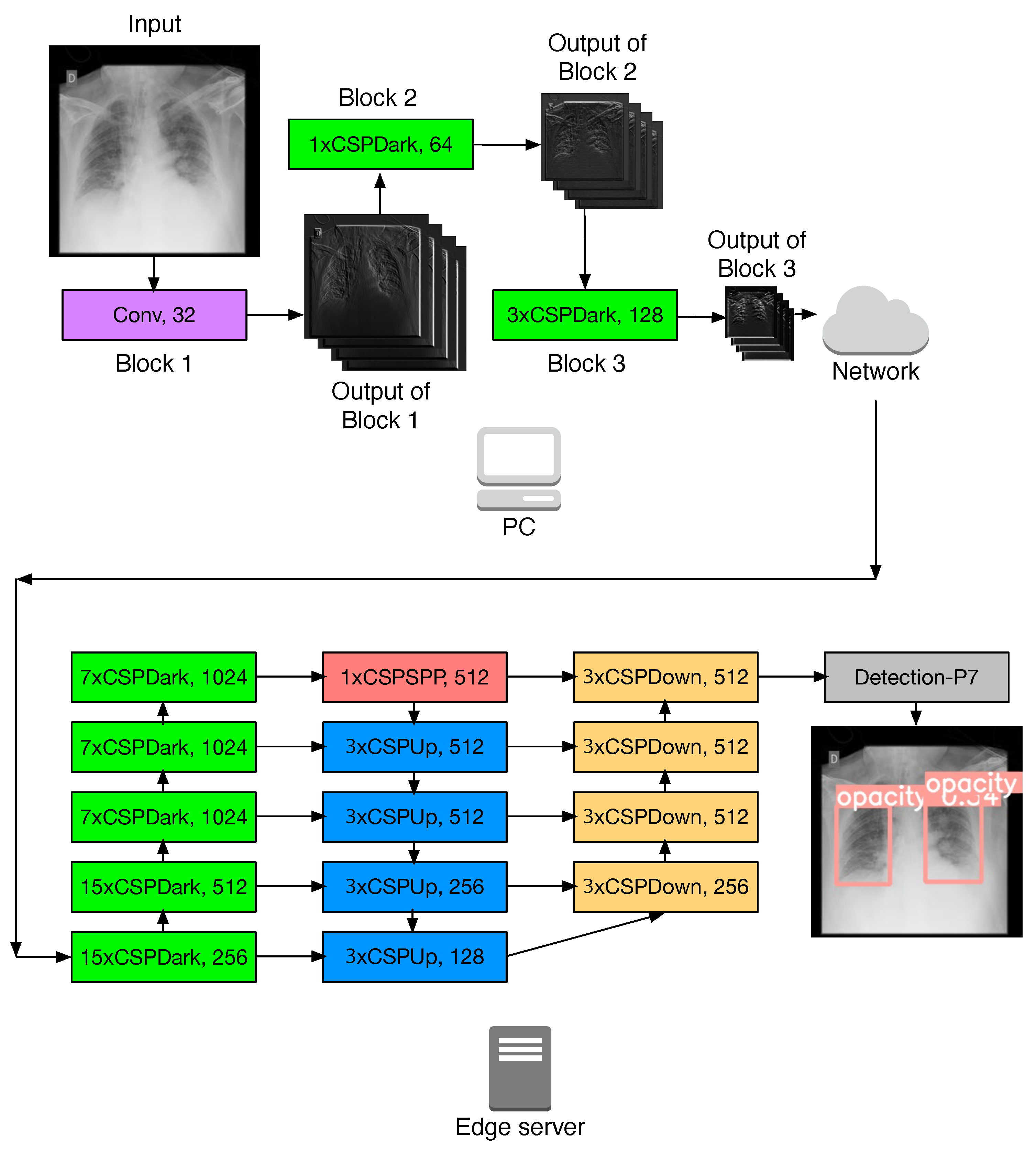
• We present BioEdge, a distributed inference framework for the bioimage object detection task. This framework can improve the throughput of the detection process in small hospitals or biomedical laboratories that lack GPU resources. It leverages the collaboration between local devices and edge servers while addressing privacy concerns.
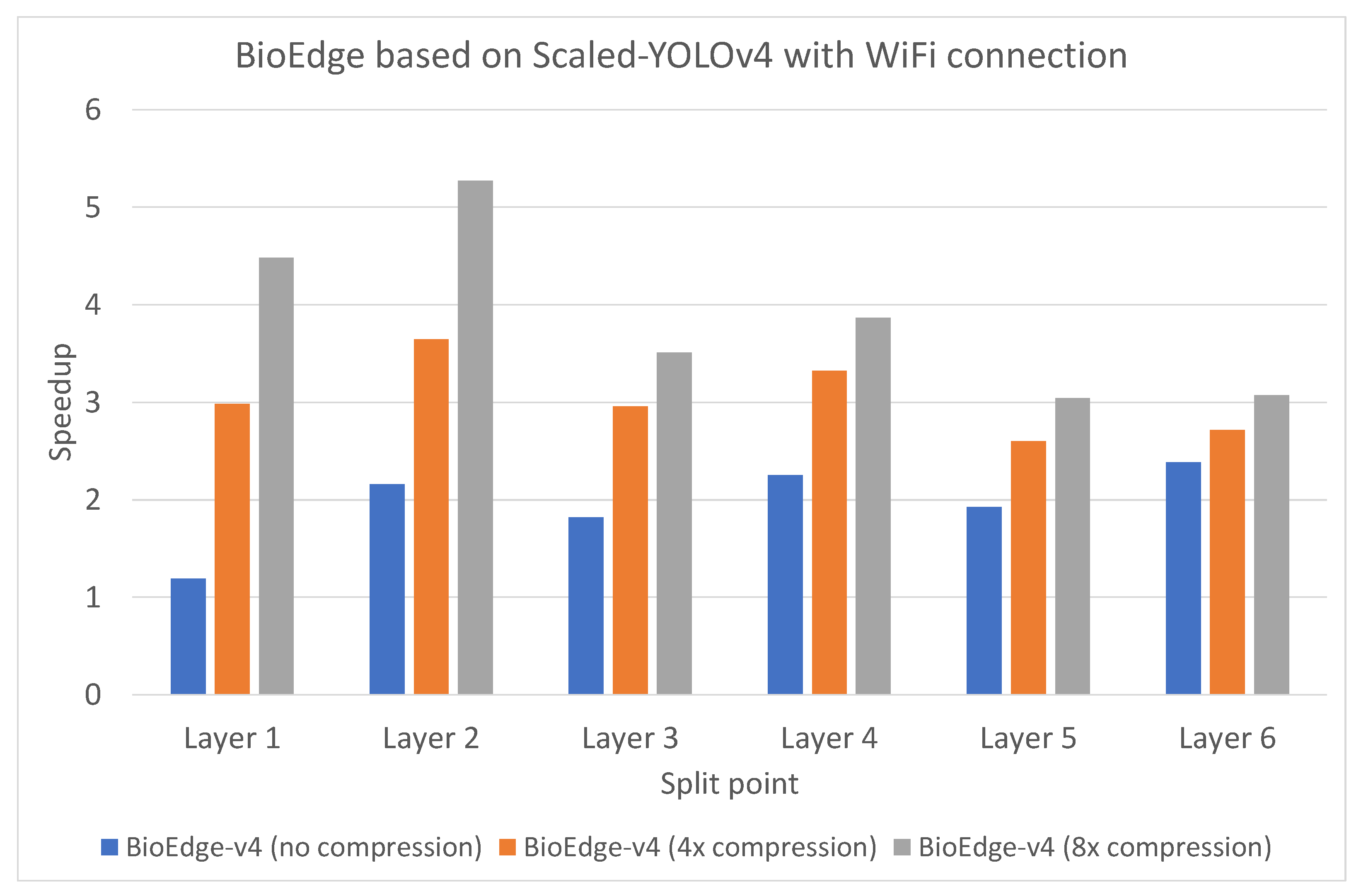
• We employ a computationally lightweight autoencoder to reduce the communication overhead when transferring data between the local device and the edge server. This autoencoder is incorporated at the distribution layer and demonstrates a negligible drop in accuracy.
• We utilize the Scaled-YOLOv4 and YOLOv7 algorithms for object detection, supporting biomedical applications that demand high accuracy. For the evaluation, we utilize the high-precision COVID-19 dataset provided by the Society for Imaging Informatics in Medicine (SIIM).

2. Related Work

Artificial intelligence (AI) is being widely used in many aspects of image classification, big data analysis, disease diagnosis, etc. [10,11]. AI approaches also accelerate advances in medical and biological research [10,12] by constructing an AI-based diagnosis system.

Typically, in AI-based diagnosis systems, the dataset is preprocessed and segmented, and the system is trained and tested before being able to classify new data [10]. Specifically, in the training phase, the input data are preprocessed. After that, important features are extracted. The preprocessing stage is necessary to preserve the inherent structure and characteristics of the original data and entails procedures to reduce noise and calibrate the image.

Deep Learning (DL) can be employed to obtain medical image data to provide indicators of molecular status, disease diagnosis, disease progression, or drug sensitivity [13]. Several DL approaches have been utilized to achieve diverse objectives, such as object segmentation, classification, disease diagnosis, and speech recognition [10].

2.1. CNN Architecture and Models

In the field of processing biomedical images such as X-ray or CT images, the popular DL technique is the convolutional neural network (CNN) [14], which was applied in 40 out of 63 studies according to a recent survey study [10]. For example, CNN accurately classified samples with breast lesion and normal samples when given medical images [15]. CNNs, a type of deep neural networks, have achieved high performance in classifying and categorizing images through the extraction of topological features of images [16]. CNNs provide the best results for large amounts of input data, but they require large amounts of data and computing resources to train [17]. When input data is limited and may not be suitable for training a CNN from scraps, a transfer learning (TL) approach can be used to harness the power of a CNN and reduce computational costs [17].

Several studies have proposed to improve performance and quality by adopting different CNN architectures. Study [18] used two CNN architectures: CSDB and CSDB-DFL. These architectures provide double residual connections between blocks, connected network links, variable-sized receive field relationships, and channel shuffling. In studies following TL approach, VGG16 [19] and AlexNet [20] are utilized for image classification tasks. In the studies, the proposed AlexNet architecture showed better performance in terms of classification accuracy compared to VGG16 [20]. Another model, OptCoNet [21], adopted a novel architecture used for feature extraction and classification tasks. The proposed system showed high performance (97.78%) in terms of accuracy. Another model, FO-MPA [22], also utilized CNN for feature extraction and adopted a marine predator algorithm (MPA) for feature selection. MPA is a nature-inspired optimization method that follows naturally occurring rules for optimal predation strategies and encounter rate policies between predators and prey in marine ecosystems. There are several studies related to COVID-19 detection. The nCOVnet citepanwar2020application used the VGG16 model for feature extraction and the TL approach in the training phase. A recent study [23] deployed a ResNet-50 network for the feature extraction task. In the study, the TL approach was used for COVID-19 detection and showed effective results compared to other related models. In another study, COVID-XNet [24] based on the DL approach showed an overall accuracy of 94.43%. Study [25] proposed a new 3D deep learning approach. The proposed approach used two classification schemes based on the ResNet-18 model and presented an overall accuracy of 86.7%. Another classification study [26] proposed a novel COVID-19 diagnostic system for classifying chest X-ray images using radioactive texture descriptors.

For the training process, in [12], two deep learning models were deployed: MobileNet V2 and SqueezeNet. The classification process was performed using the support vector machine (SVM) technique, and it showed an overall accuracy of 99.27%. Another study [27] used the ResNet50 model for feature extraction and refinement tasks and SVM for the classification process, achieving an overall accuracy of 99.29%. In another study, COVIDiagnosis-Net [28] proposed a new system model based on Bayes-SqueezeNet.

Deep transfer learning (DTL) [29,30] has also been adopted in several studies. The DTL approach can be used to overcome the overfitting and underfitting problems of small training input data by utilizing the benefits of CNNs that are first trained using large input data [19]. Study [31] deployed DTL techniques using two models, GoogleNet and AlexNet. The models were evaluated in different contexts and showed promising results. Several deep learning models, namely VGG19, VGG16, Inception-ResNet-V2, InceptionV3, DenseNet121, Xception, and Resnet50, were used in a comparative study by Shazia et al. [32]. Among the deployed models, the best performing model in terms of classification accuracy was DenseNet121.

2.2. Biomedical Image Preprocessing and Augmentation

Image preprocessing can improve the quality and size of images in biomedical datasets [33]. Several procedures can be performed to achieve goals such as reducing noise in the initial image, enhancing quality by increasing contrast, and removing high/low frequencies [34]. This entails converting an insufficient dataset into a sufficient dataset. Several transformations can be applied to a dataset, such as scaling, cropping, flipping, filtering, and rotating, so that each image can be transformed into a new image that contains the information needed to proceed to the next step. Grayscaling can also be applied to initial datasets because they are usually generated by different types of machines. Therefore, a histogram matching procedure can be performed on all samples by considering one sample as a reference to unify the histogram distribution of all samples [24]. Lack of data or unreliable data can affect the effectiveness of ML and DL due to lack of sufficient features [35].

The overfitting problem occurs when a network learns a task with very large variance, such as perfectly modeling the training data [19,36]. These model variants typically involve noise, contrast changes, rotation, and translation. In biased inputs, data augmentation can be utilized to increase the number of rare samples. In data augmentation, common sources of variation are specifically added to the training data. The data augmentation approach is beneficial for even small medical image processing [10].

Data augmentation consists of a set of approaches that improve the quality and size of the training dataset to enable a better DL system to be utilized. Data augmentation is typically addressed using generative adversarial neural networks (GANs) [37,38]. Several studies have considered GANs as a useful tool for data augmentation [37]. However, many types of GANs can suffer from instability in training phase and falling into gradient saturation. Several studies [18,25,39,40] utilized an image augmentation approach to increase the number of images in the initial dataset. Studies using augmented datasets [26] have shown significant improvements in system performance compared to systems using initial datasets.

2.3. Distributed Inference

Distributed inference can augment the limited computational capabilities of a local device by utilizing both the local device and a GPU server. Neurosurgeon [41] first introduced partitioning and distribution strategies with layer-by-layer investigation using a mobile device and a cloud server. It has been demonstrated that distributed inference is advantageous for resource-limited devices.

Recent studies in the field of distributed inference for object detection using machine learning have focused on enhancing the efficiency and accuracy of object detection algorithms. One approach is to distribute the inference between two nodes, such as a mobile device and the cloud, while considering communication rate constraints. This process entails transmitting a description of the observed variable to the cloud, which subsequently computes an estimate of the target variable [42]. Furthermore, efforts have been made to exploit object-to-object relationships during learning by employing graph convolutional networks (GCNs) to construct a relation graph that encodes both geometric and visual relationships between objects [43]. These recent studies aim to enhance the performance of distributed inference in object detection using machine learning techniques.

In an edge computing environment, communication overhead between the local device and the edge server is often a bottleneck. To address this issue, Bottlenet++ [44] introduced an encoding method at the partitioning point to reduce the size of transferred data. To compress the data, the authors adopted JPEG methods with quantization for further encoding. It is important to note that this encoding method itself consumes processing time, so if it is computationally complex, it can also become a bottleneck. In contrast, BioEdge carefully designed the autoencoder with a simple convolution-transposed convolution pair to reduce the overall data communication overhead.

Several studies have adopted distributed inference for object detection. In previous studies [45,46], the Faster R-CNN object detection algorithm was applied to biomedical data for disease diagnosis. However, this algorithm exhibited lower accuracy when compared to Scaled-YOLOv4 or YOLOv7. Smaller-scale object detection models, such as YOLOv4-tiny, can be utilized for resource-limited devices. However, they suffer a significant accuracy drop in order to achieve acceptable inference times on performance-limited resources [6].

In contrast to existing research, BioEdge adopts the state-of-the-art object detection algorithm specifically designed for the demanding biomedical field, where high accuracy is essential.

3. BioEdge

In this section, we provide a detailed explanation of the methods used in BioEdge.

3.1. Dataset Preparation

In this study, we used the COVID-19 X-ray image dataset from the Kaggle SIIM-FISABIO-RSNA COVID-19 Detection competition [9]. The dataset comprises 6334 Chest X-ray scan images that are annotated with bounding boxes and classified for abnormalities by experienced radiologists. To work with these data, it is necessary to first convert them from the Digital Imaging and Communications in Medicine (DICOM) format to the PNG format. Subsequently, we resized the images to 896 × 896 pixels, a dimension known to yield high accuracy for Scaled-YOLOv4 [6] and YOLOv7 [7].

The bounding box labels, representing the rectangular location of the objects in the images, need to be converted to YOLO annotation. YOLO annotation consists of $x_{center}$, $y_{center}$, $width$, and $height$, representing normalized coordinate values for the bounding box location. Given that the data provide $x_{min}$, $y_{min}$, $x_{max}$, and $y_{max}$ values for the bounding box, the computations can be expressed as follows:

$$\begin{array}{cc}\hfill width& =(x_{max}-x_{min})/IMG\_SIZE\hfill \\ \hfill height& =(y_{max}-y_{min})IMG\_SIZE\hfill \\ \hfill x_{center}& =(x_{min}+width/2)IMG\_SIZE\hfill \\ \hfill y_{center}& =(y_{min}+height/2)IMG\_SIZE\hfill \end{array}.$$

(1)

$IMG\_SIZE$ represents the size of the image. This value is used to scale and normalize coordinate values within the range of 0 to 1. As previously mentioned, we set $IMG\_SIZE$ to 896.

To demonstrate the stability of the utilized model, we performed cross-validation. We divided the complete dataset into 5 subsets and carried out 5 iterations, employing each subset alternately for both validation and training to ensure that each subset was used for validation at least once. The accuracy results from these iterations were then averaged.

3.2. Scaled-YOLOv4

Object detection is a task that involves identifying objects within an image and representing their locations using bounding boxes. To tackle this task, deep learning employs two types of approaches. The first is two-stage object detection. In this approach, the system initially identifies candidate bounding boxes, assuming the presence of objects. These candidates then pass through a Convolutional Neural Network (CNN) for classification, determining whether they indeed contain an object or not. Representative two-stage approaches include R-CNN, Fast R-CNN, and Faster R-CNN. The other approach is one-shot object detection. YOLO is a representative one-shot object detection approach that determines the probability of each object’s existence within a single bounding box.

Scaled-YOLOv4 [6] is a state-of-the-art object detection algorithm that introduces a network scaling approach based on the YOLOv4 object detection neural network, employing the cross-stage partial (CSP) approach. This approach moves beyond modifying the depth, width, and resolution; it also restructures the network’s architecture to optimize both speed and accuracy for networks of varying sizes. In their work, the authors of [6] delve into the upper and lower bounds of linear scaling for upscaling and downscaling models and conduct a detailed analysis of critical considerations in model scaling, addressing the needs of both small and large models.

In the context of edge computing, it is crucial to carefully consider effective scaling, as it can impose constraints on the adaptability of the network to various scenarios. For instance, a network optimized for achieving high accuracy with large datasets may not be well-suited for real-time applications demanding swift processing and minimal latency. Conversely, a network tailored for low-power devices might not be adequate for high-performance computing environments. Given the mixed nature of scenarios in edge computing, it becomes imperative to contemplate scaling both up and down during neural network design to ensure their relevance and applicability within edge computing environments. Thus, we adopt the scaled-YOLOv4 method as our object detection algorithm because a powerful model scaling method is required in the edge computing environment.

3.3. YOLOv7

YOLOv7 [7] is a real-time object detection system that surpasses all known object detectors in terms of both speed and accuracy. It achieves the highest accuracy of 56.8% average precision (AP) among all known real-time object detectors with 30 FPS or higher on GPU V100. YOLOv7 introduces trainable bag-of-freebies modules and optimization methods to improve the accuracy of object detection without increasing the inference cost. The authors propose a compound scaling method that involves scaling up the depth of computational blocks by 1.5 times and the width of transition blocks by 1.25 times. This method improves the AP by 0.5 with fewer parameters and computation compared to methods that only scale up the width or the depth.

YOLOv7-E6, a specific variant of YOLOv7, outperforms other object detectors like SWIN-L Cascade-Mask R-CNN and ConvNeXt-XL Cascade-Mask R-CNN in terms of both speed and accuracy. It is 509% faster than SWIN-L Cascade-Mask R-CNN and 551% faster than ConvNeXt-XL Cascade-Mask R-CNN, while also achieving higher accuracy.

Compared to previous versions like YOLOv4 and YOLOR-CSP, YOLOv7 has fewer parameters and computation requirements while achieving higher AP. It also performs well in the tiny model and cloud GPU model scenarios. In terms of model size, YOLOv7 has 36.9 million parameters and 104.7 billion FLOPs, making it a relatively large and computationally intensive model. It has a size of 640 and achieves a frame rate of 161 FPS on the V100 GPU.

3.4. Overall Design of BioEdge

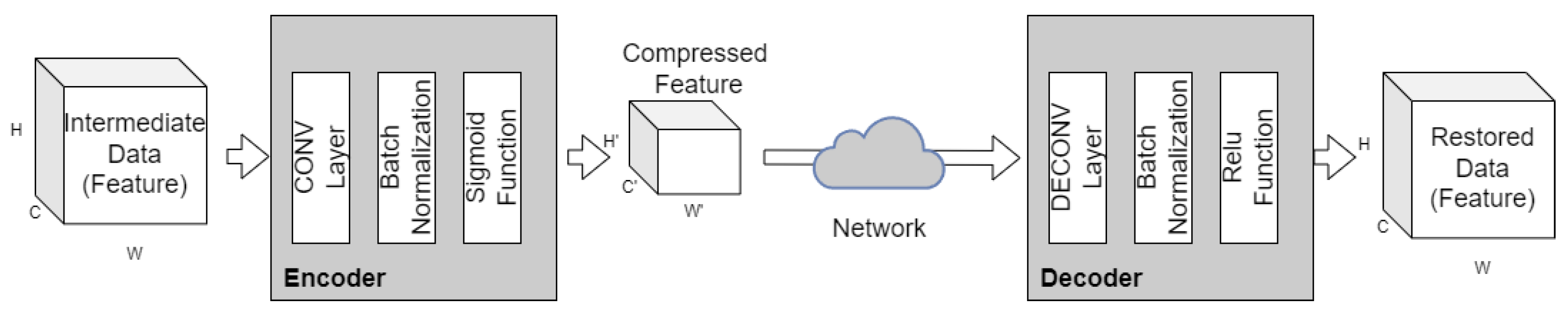
Figure 1 illustrates the overall design of the proposed framework. The fundamental concept of BioEdge is division of an object detection task into two components and allocation of each task to both the local computer and the edge server, which is equipped with a powerful GPU. For object detection, BioEdge employs Scaled-YOLOv4 [6] and YOLOv7 [7], cutting-edge object detection algorithms. These algorithms represent an enhanced version of YOLO and incorporates a model scaling technique that adjusts the depth, width, resolution, and structure of the network to achieve higher accuracy. In addition, BioEdge utilizes the SIIM COVID-19 dataset [9], which includes 6334 chest scan images meticulously labeled by an international group of radiologists.

Figure 1. Overall architecture of BioEdge. Scaled-YOLOv4 used in BioEdge consists of CSPDark, CSPSPP, CSPUp, and CSPDown blocks.

In the following, we explain the process of setting the split points for Scaled YOLOv4 and YOLOv7 for distributed inference. Due to the significant structural differences between these two models, we describe the division process for each model separately.

Scaled-YOLOv4: Scaled-YOLOv4 comprises CSPDark, CSPSPP, CSPUp, and CSPDown blocks, as depicted in Figure 1. Each CSP block is a reconfigured convolutional neural network block built upon the Cross-Stage Partial Network (CSPNet) concept [47], aimed at reducing the number of parameters while enhancing accuracy.

In the context of model slicing, our approach commences with a profiling of Scaled-YOLOv4 to identify potential slicing points. It is noteworthy that Scaled-YOLOv4 incorporates various computational blocks with skip connections, enabling each block to bypass several intermediate blocks and establish connections with blocks adjacent to the skipped ones. However, we do not consider these skip connection blocks as suitable slicing points due to the additional network transfer overhead they would introduce.

As illustrated in Figure 1, we identify the first three blocks as feasible slicing points within Scaled-YOLOv4. Furthermore, upon closer examination, we identify an additional potential slicing point within each block, resulting in a total of six feasible slicing points. Next, we proceed to generate all possible partitioned models, systematically incrementing the split point from one to six, facilitating benchmarking at each split point. In each partitioned model, we optionally include an autoencoder responsible for encoding the data intended for transfer to the edge and decoding the data upon arrival at the edge server. This is explained in more detail in Section 3.5. Subsequently, we benchmark these partitioned models on real hardware, encompassing both a PC and the edge server, which allows for measuring the inference latency for each partitioned model. Finally, we deploy the partitioned model that demonstrates the best performance onto both the PC and the edge server.

YOLOv7: To facilitate model slicing, we initially profile YOLOv7. YOLOv7 has a different model structure compared to Scaled-YOLOv4, which means we cannot directly use the slicing points taken from Scaled-YOLOv4. Like Scaled-YOLOv4, YOLOv7 also includes computational blocks structured with skip connections. These skip connections are intricately interwoven, making it slightly challenging to determine the slicing points in YOLOv7. Figure 2 illustrates the early layers of YOLOv7. In YOLOv7, among the various supported models, we utilize the e6e model, which has the highest accuracy.

Figure 2. Early layers of YOLOv7 used in BioEdge.

The first split point in the figure, marked as the first split point, is the first layer that can be split and is a Concat block. This block takes four inputs and produces one output, making it suitable as a split point. The next potential split point, marked as the second split point, is a Mul block that takes two inputs and produces two identical outputs. In this case, as the output contents are the same, BioEdge sends only one output to the edge server and, within the edge server, replicates the output and sends it to subsequent layers. The third potential split point is another Concat block, similar to the second split point, sending the same single output to the edge server, where it is copied and distributed to four parallel layers.

Using this approach, we identify a total of six split-capable layers without skip connections. Similar to Scaled-YOLOv4, we conduct performance evaluations in a real PC and edge server environment for all these split-capable layers, selecting the optimal layer with the best latency as the split point.

Inference: During bioimage analysis, BioEdge on the local computer takes a bioimage as input and performs the neural network layers of Scaled-YOLOv4 or YOLOv7 up to the designated slicing point using its local CPU. Subsequently, the output data at the split point are transmitted to the edge server via the network. If an autoencoder is employed, as elaborated in Section 3.5, the output data at the split point undergo compression, typically achieving a reduction in size by a factor of 4 or 8. Despite the data compression applied by BioEdge to reduce network traffic, our autoencoder implementation, consisting of an encoder and a decoder within a neural network, results in only a negligible decrease in accuracy.

In the edge server, BioEdge forwards the received data to the initial layer of the remaining Scaled-YOLOv4 or YOLOv7 models situated on the edge. In case an autoencoder is utilized, BioEdge restores the compressed data to their original form by employing the decoder. Following the completion of the inference task executed with a GPU, the results are relayed back to the local PC through the reverse path. BioEdge is implemented using PyTorch and the NVIDIA Triton Inference Server.

BioEdge prioritizes privacy enhancement. A recent study advocating for a privacy-preserving medical platform highlights that as a medical image traverses a limited number of DNN layers, distinguishing specific data items within the processed image becomes challenging [8]. This difficulty arises because the convolutional and max pooling operations introduce non-linear and non-reversible effects to the image. By transmitting the processed intermediate representations of bioimages which underwent these convolutional and max pooling operations to the edge instead of the original bioimages, BioEdge significantly augments data privacy.

3.5. Autoencoder

Data compression is essential in device-edge co-inference systems to alleviate communication overhead and on-device computation. In distributed inference, a neural network is partitioned at the mobile device, and the intermediate features generated by the network’s initial segment are transmitted to the edge server for further processing. Although these intermediate features are smaller than the input data, they can still be substantial enough to introduce communication overhead and on-device computation challenges. Utilizing data compression reduces the size of intermediate data, facilitating their transmission over the network.

In BioEdge, data compression is achieved through the utilization of an autoencoder, comprising an encoder and decoder. To minimize the operational overhead of the autoencoder, we employ a lightweight autoencoder consisting of a single convolution layer and a transposed convolution layer. Figure 3 illustrates our data compression architecture, with a primary focus on feature data. The compression of features relies on the inherent sparsity and fault-tolerant properties of intermediate features within deep neural networks. The encoder effectively compresses the intermediate feature by leveraging its sparsity and reducing its dimensionality. This reduction is achieved through a lossy compression process. The convolutional layer dynamically adjusts the number of filters to manage the quantity of output channels, while the stride of the convolutional operation and the size of the kernel determine the width and height of the output feature. Specifically, the intermediate feature data can be represented as a tensor with three dimensions: channel, width, and height. Subsequently, the decoder works to reconstruct the compressed feature at the edge server.

Figure 3. Data compression architecture of BioEdge.

The key operations in the encoder/decoder are explained as follows:

• A convolutional (CONV) layer performs a convolution operation on the input data. The convolution operation involves sliding a small filter over the input data and computing the dot product between the filter and the input at each position. The result of the convolution operation is a feature map that captures the presence of certain features in the input data. In the encoder, the convolutional layers are used to extract features from the input data and create a compressed representation of the data.
• Batch normalization involves normalizing the inputs to a layer by subtracting the mean and dividing by the standard deviation. This helps to reduce the internal covariate shift, which is a phenomenon where the distribution of the inputs to a layer changes during training. By reducing the internal covariate shift, batch normalization helps to stabilize the training process and improve the performance of the network. In the encoder, the batch normalization layer is used to normalize the inputs to the convolutional layers and improve the training process.
• A deconvolutional (DECONV) layer, also known as a transposed convolutional layer, performs an inverse convolution operation on the input data. The deconvolution operation involves sliding a small filter over the input data and computing the dot product between the filter and the input at each position. The result of the deconvolution operation is a feature map that captures the presence of certain features in the input data. In the decoder, the deconvolutional layers are used to reconstruct the original data from the compressed representation created by the encoder.
• The Sigmoid function is an activation function that maps any input value to a value between 0 and 1. In the encoder, the Sigmoid function is used in the last layer of the encoder. Because the output values are constrained to the range [0, 1] in the Sigmoid function, the values can be scaled to satisfy the transmitter output power constraint. Namely, the output values can be adjusted to fit within a certain power budget, which is important in resource-constrained mobile devices where power consumption is a critical factor. It also benefits the quantization of data in the digital communication system. Quantization is the process of mapping a continuous range of values to a finite set of discrete values, which is necessary for transmitting data over the network. By constraining the output values to [0, 1], the quantization process can be simplified and made more efficient, further reducing communication overhead and improving the overall performance of the system.
• The ReLU (Rectified Linear Unit) function is an activation function that maps any input value less than 0 to 0, and any input value greater than 0 to the same value. In the decoder, the ReLU function is used in the first layer of the decoder. The ReLU function is well-suited for tasks that involve detecting and extracting features from data. The ReLU function helps to activate the relevant features in the data and suppress the irrelevant features.

4. Results

We present the performance evaluation results of BioEdge in this section.

4.1. Experimental Environment

We implemented BioEdge with a laboratory PC and an Edge server environment. As a local laboratory PC, we used an Intel i5-7500 platform with four 3.40 GHz cores and 16 GB of RAM. The edge server employs an Intel i7-10700 CPU, which has eight 2.8 GHz cores, 32 GB of RAM, and an NVIDIA GeForce RTX 3090 GPU with 24 GB of memory. The local PC and edge server is directly connected with the 1 GbE switch. The network performance was configured as 1 Gbps for the LAN environment and 500 Mbps for the WiFi environment. The 500 Mbps setting was configured using the TC (Traffic Control) application in Linux. We utilized the SIIM COVID-19 dataset [9] for inference and training. The chest image size is 512 × 512 × 3 pixels. Our training model uses Adam optimizer with the learning rate of 0.0001.

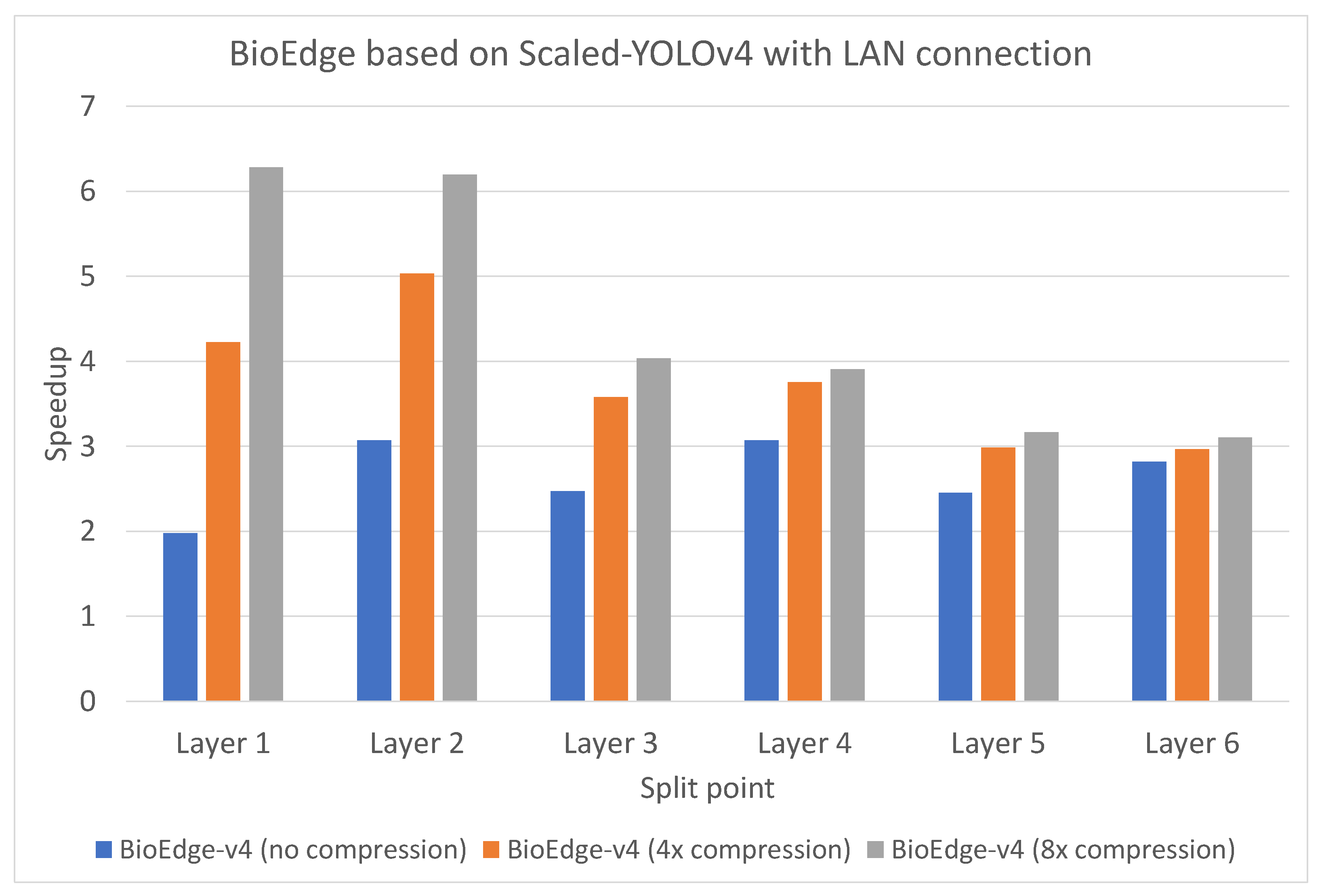
4.2. Inference Latency

To obtain the speedup value of BioEdge compared to the execution speed using only the Local PC, we performed the inference task 20 times and calculated the average value. The speed-up value was calculated using the standard speed-up formula, where it represents the ratio of the time taken on a local PC to the time taken when running BioEdge.

Scaled-YOLOv4: We first evaluated BioEdge based on Scaled-YOLOv4, referred to as BioEdge-v4. Figure 4 illustrates the speedup of uncompressed BioEdge and BioEdge with fourfold and eightfold compression through an autoencoder, compared to using only the Local PC, when the network bandwidth is 1 Gbps in an LAN environment. The performance improvement is illustrated for various potential slicing points of Scaled-YOLOv4. For BioEdge without the application of an autoencoder, slicing the DNN model at Layer 4 resulted in a substantial speedup of 3.08, while slicing at Layer 2 yielded a speedup of 3.07. In the case of BioEdge without autoencoder application, the DNN model’s accuracy remained unaffected, making it suitable for accuracy-critical application environments. In BioEdge, to achieve higher inference latency, a slight trade-off in accuracy can be tolerated by utilizing an autoencoder to compress and restore transmitted data. BioEdge with a fourfold compression through the autoencoder showed the highest speedup value of 5.03 at Layer 2 compared to using only the Local PC, followed by a speedup value of 4.22 at Layer 1. For BioEdge with an eightfold compression, the highest speedup value of 6.28 was observed at Layer 1 compared to using only the Local PC, followed by a speedup value of 6.19 at Layer 2.

Figure 4. Speedup value of BioEdge based on Scaled-YOLOv4 (BioEdge-v4) when the network connection is LAN with 1 Gbps.

Figure 5 displays the speedup values of uncompressed BioEdge, BioEdge with fourfold compression through autoencoder, and BioEdge with eightfold compression through autoencoder in a Wi-Fi environment with a bandwidth of 500 Mbps. For the uncompressed BioEdge, the highest performance improvement of 2.38 in speedup was achieved when cutting Scaled-YOLOv4 at Layer 6, followed by a speedup of 2.25 when cutting at Layer 4. BioEdge with fourfold compression showed the highest performance improvement of 3.64 at Layer 2, followed by a performance improvement of 3.32 at Layer 4. With eightfold compression, BioEdge exhibited performance improvements of 5.27 at Layer 2 and 4.48 at Layer 1.

Figure 5. Speedup value of BioEdge based on Scaled-YOLOv4 (BioEdge-v4) when the network connection is Wifi with 500 Mbps.

YOLOv7: We evaluated BioEdge based on YOLOv7 next, referred to as BioEdge-v7. Figure 6 shows the speedup of uncompressed BioEdge and BioEdge with fourfold and eightfold compression through an autoencoder in a 1 Gbps network bandwidth environment. Speedup indicates how much faster BioEdge is compared to the Local PC. In Scaled-YOLOv4, it was possible to sequentially select each layer as a slicing point from the front. However, YOLOv7 has a more complex structure as shown in Figure 2, making it impossible to select slicing points sequentially. In YOLOv7, the layers that can be sliced are marked as Point 1 through 6, corresponding to Layers 40, 43, 54, 111, 122, and 179, respectively.

Figure 6. Speedup value of BioEdge based on YOLOv7 (BioEdge-v7) when the network connection is LAN with 1 Gbps.

BioEdge without the application of the autoencoder showed a significantly high speedup of 9.20 at Point 1. Following that, it exhibited the next highest speedup of 3.15 at Point 3. For the remaining Points, it displayed speedups in the range of 1.61 to 2.42. YOLOv7 had a total of 1049 layers, and at Point 1, it offloaded most of the processing to the edge server, allowing for making efficient use of the edge server’s GPU resources, resulting in high performance. Point 2 is also in the early layers, adjacent to Point 1, but it did not achieve the same level of speedup as Point 1 because of the higher data transfer volume compared to Point 1.

When applying a 4× compression with the autoencoder, BioEdge showed a speedup of 11.02 at Point 1, making it perform even faster than the uncompressed BioEdge. The second highest performance was at Point 3 with a speedup of 5.32, and the third highest was at Point 2 with a speedup of 4.19. Even at Point 2, which has a high data transfer volume, compression techniques helped achieve a higher speedup compared to the uncompressed case. With eightfold compression using the autoencoder, BioEdge showed a speedup of 12.15 at Point 1, outperforming the fourfold compressed BioEdge. The secondchighest performance was at Point 2 with a speedup of 6.83, and the third highest was at Point 3 with a speedup of 6.01. When compressing by eightfold, the reduction in data transfer volume at Point 2 allowed it outperformance of Point 3. This demonstrates the efficiency of compression in layers with high data transfer volume.

Figure 7 displays the speedup of an uncompressed BioEdge, BioEdge with fourfold compression through an autoencoder, and BioEdge with eightfold compression through an autoencoder in a 500 Mbps network bandwidth environment. In the case of the uncompressed BioEdge, the most substantial performance enhancement, with a speedup of 9.18, was realized by splitting YOLOv7 at Point 1, followed by a speedup of 3.11 when dividing at Point 3. For BioEdge with fourfold compression, the most significant performance improvement occured at Point 1, achieving a speedup of 10.84, and Point 2 exhibited a performance enhancement of 5.29. When applying eightfold compression, BioEdge showcased remarkable performance improvements, achieving a speedup of 12.15 at Point 1 and 6.97 at Point 2.

Figure 7. Speedup value of BioEdge based on YOLOv7 (BioEdge-v7) when the network connection is Wifi with 500 Mbps.

Summary: These significant speedup results underscore the efficiency of BioEdge using distributed inference, particularly in settings such as GPU-lacking laboratories or hospital environments. BioEdge efficiently executes the Scaled-YOLOv4 or YOLOv7 model by running the layers of the model after the split point on an edge server equipped with a GPU. Moreover, it enhances security by transmitting intermediate representations processed through convolution layers to the edge server rather than sending the original images directly. Even in BioEdge without the application of an autoencoder, it demonstrates notable improvements. However, for BioEdge with eightfold compression, it exhibits a significant performance enhancement compared to uncompressed BioEdge. This illustrates that data transmission becomes a bottleneck in distributed inference, and it becomes evident that applying data compression is efficient, even with a slight trade-off in accuracy.

4.3. Inference Accuracy

Using an autoencoder to compress transmitted data and reduce the amount sent to the edge server is effective in reducing the overall inference time. However, due to data modifications caused by the autoencoder, this approach can lead to a decrease in accuracy compared to sending the original data. Table 1 presents the mean average precision (mAP) scores of the original Scaled-YOLOv4 executed on a local PC, uncompressed BioEdge, and BioEdge with fourfold and eightfold compression. Uncompressed BioEdge processes the same data as the original Scaled-YOLOv4 at each layer, thus maintaining the same level of accuracy. However, both fourfold and eightfold compressed BioEdge models exhibit slight accuracy degradation due to the applied compression. Nevertheless, the decline in mAP scores is not substantial, and the mAP scores are competitive compared to other algorithms that achieved impressive results in the SIIM COVID-19 dataset competition [48].

Table 1. Accuracy of original Scaled-YOLOv4, uncompressed BioEdge, and BioEdge with 4-fold and 8-fold compression.

Framework	Accuracy (mAP50)
Original Scaled-YOLOv4	0.543
BioEdge (no compression)	0.543
BioEdge (4-fold compression)	0.541
BioEdge (8-fold compression)	0.540

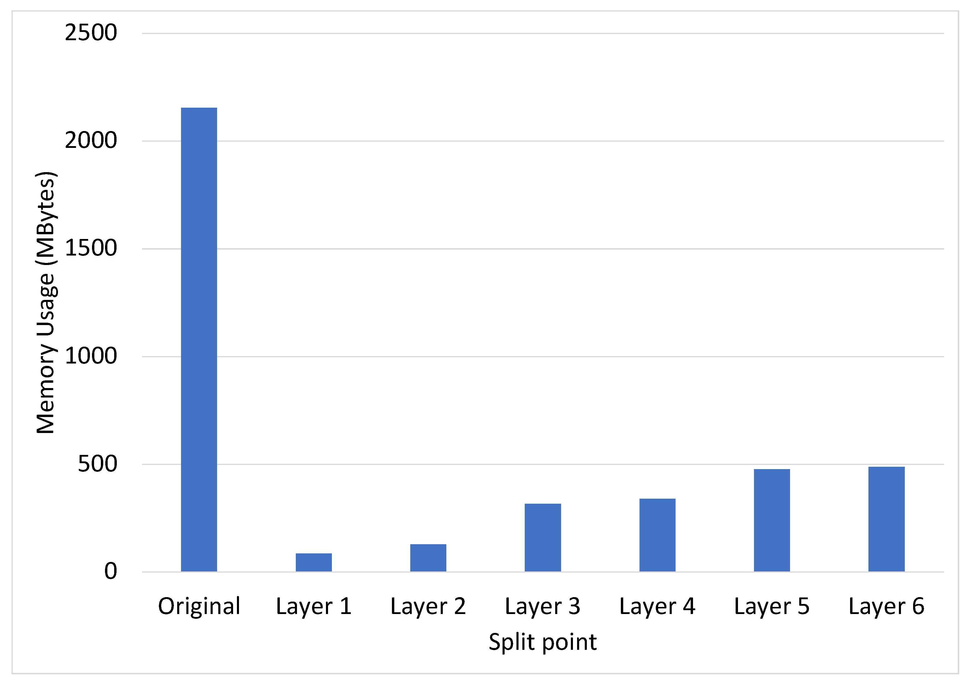
4.4. Memory Consumption

BioEdge offers the advantage of reducing memory usage on the local PC by performing only the front layers of Scaled-YOLOv4 through distributed inference, thus avoiding the need to allocate memory space for the entire model. Figure 8 illustrates the memory usage on the local PC when executing all layers of Scaled-YOLOv4 and when using BioEdge to split the model at each layer. When executing all layers of Scaled-YOLOv4 on the local PC, a memory capacity of 2154 MB is required. In contrast, when using BioEdge, the memory usage starts at 87 MB in Layer 1 and increases to 489 MB in Layer 6, showcasing efficient memory utilization. This implies that using BioEdge allows for the use of lower-spec local PCs without issues, offering the advantage of running various different deep learning models simultaneously.

Figure 8. Memory usage of BioEdge on the local PC at each split point.

5. Discussion

In this section, we discuss the strengths and weaknesses of BioEdge, as well as future work in relation to it.

Comparing with general image datasets: The focus of this paper remained on bioinformatics, and we exclusively employed bioimages as our dataset. The key distinction between the bioimages we utilized and other image types lies in the channels. Bioimages captured with equipment such as X-ray and CT are typically single-channel grayscale images, whereas general images are commonly color images, composed of three channels. Adjustments to the input layer of the target model are necessary when changing the number of channels. Furthermore, training the model with grayscale X-ray or CT images requires a diverse range of images with various tissues, densities, and resolutions for effective learning. In contrast, training with general images involves a variety of colors, patterns, and objects.

Comparing with model compression: Using techniques such as pruning to employ lightweight models can inherently enhance model performance. According to prior research [49], when pruning is applied to ResNet50, it results in less than a 1% drop in accuracy and a 41.8% reduction in FLOPs (Floating-Point Operations). With a 41.8% decrease in FLOPs, the anticipated speedup when using a lightweight model on a local PC is expected to be less than two. In contrast, BioEdge, leveraging high-performance GPUs in edge computing, achieves an even higher speedup.

Automated profiling tool: The drawback of BioEdge is that when applying a new object detection model, we need to manually analyze the model to find the optimal split point. As for future work, there is a need to develop tools that can automatically find the split point for new models. Such a tool can be implemented using either an estimation-based approach or a benchmark approach.

Improving security: BioEdge currently maintains a relatively high level of security since it sends the intermediate representation, which is transformed by convolutional layers, to the edge server. Nevertheless, encrypting the data sent over the network and decrypting it at the edge server can further enhance security. This approach ensures that the intermediate representation remains confidential until decryption in the server’s memory. We plan to integrate data encryption and decryption into BioEdge.

Real medical settings: It is essential to demonstrate the real-world effectiveness of BioEdge by applying it in actual medical environments. We plan to collaborate with medical professionals who are interested in this field to conduct research involving the practical application of BioEdge in real medical environments.

Broader datasets: BioEdge can be applied not only to object detection but also to the field of disease segmentation. The SIIM organization, which provided the COVID-19 dataset we used, also offers various other datasets. These include SIIM-ISIC Melanoma Classification and SIIM-ACR Pneumothorax Segmentation. We plan to include these datasets in our future research.

6. Conclusions

Deep learning-based computer vision technologies have enabled effective bioimage analysis for disease diagnosis. However, these deep learning algorithms require a substantial amount of computational resources during inference. Consequently, performing inference tasks in a laboratory or hospital without in-house GPU facilities poses a significant challenge.

In this study, we introduced BioEdge, a framework designed to accelerate object detection in bioimages by employing a distributed inference technique with Scaled-YOLOv4 and YOLOv7. We demonstrated that BioEdge significantly enhances the performance of Scaled-YOLOv4 and YOLOv7 through the utilization of edge computing. We illustrated the practicality of BioEdge by applying it solely to the COVID-19 dataset. Nevertheless, BioEdge can be readily adapted to other bioimage object detection tasks. We plan to evaluate BioEdge with various bioimage datasets collected for disease diagnosis.

References

1. Min, S.; Lee, B.; Yoon, S. Deep learning in bioinformatics. Brief. Bioinform. 2017, 18, 851–869. [Google Scholar] [CrossRef] [PubMed]
2. Cruz-Roa, A.; Gilmore, H.; Basavanhally, A.; Feldman, M.; Ganesan, S.; Shih, N.N.; Tomaszewski, J.; González, F.A.; Madabhushi, A. Accurate and reproducible invasive breast cancer detection in whole-slide images: A deep learning approach for quantifying tumor extent. Sci. Rep. 2017, 7, 46450. [Google Scholar] [CrossRef]
3. Kim, Y.; Yi, S.; Ahn, H.; Hong, C.H. Accurate Crack Detection Based on Distributed Deep Learning for IoT Environment. Sensors 2023, 23, 858. [Google Scholar] [CrossRef] [PubMed]
4. Robinson, T.; Harkin, J.; Shukla, P. Hardware acceleration of genomics data analysis: Challenges and opportunities. Bioinformatics 2021, 37, 1785–1795. [Google Scholar] [CrossRef]
5. Hong, C.H.; Varghese, B. Resource management in fog/edge computing: A survey on architectures, infrastructure, and algorithms. ACM Comput. Surv. (CSUR) 2019, 52, 1–37. [Google Scholar] [CrossRef]
6. Wang, C.Y.; Bochkovskiy, A.; Liao, H.Y.M. Scaled-yolov4: Scaling cross stage partial network. In Proceedings of the IEEE/CVF Conference on Computer Vision and Pattern Recognition, Virtual. 19–25 June 2021; pp. 13029–13038. [Google Scholar]
7. Wang, C.Y.; Bochkovskiy, A.; Liao, H.Y.M. YOLOv7: Trainable bag-of-freebies sets new state-of-the-art for real-time object detectors. In Proceedings of the IEEE/CVF Conference on Computer Vision and Pattern Recognition, Vancouver, BC, Canada, 17–24 June 2023; pp. 7464–7475. [Google Scholar]
8. Ha, Y.J.; Yoo, M.; Lee, G.; Jung, S.; Choi, S.W.; Kim, J.; Yoo, S. Spatio-Temporal Split Learning for Privacy-Preserving Medical Platforms: Case Studies With COVID-19 CT, X-ray, and Cholesterol Data. IEEE Access 2021, 9, 121046–121059. [Google Scholar] [CrossRef]
9. Lakhani, P.; Mongan, J.; Singhal, C.; Zhou, Q.; Andriole, K.P.; Auffermann, W.F.; Prasanna, P.; Pham, T.; Peterson, M.; Bergquist, P.J.; et al. The 2021 SIIM-FISABIO-RSNA Machine Learning COVID-19 Challenge: Annotation and Standard Exam Classification of COVID-19 Chest Radiographs. J. Digit. Imaging 2023, 36, 365–372. [Google Scholar] [CrossRef]
10. Abumalloh, R.A.; Nilashi, M.; Ismail, M.Y.; Alhargan, A.; Alghamdi, A.; Alzahrani, A.O.; Saraireh, L.; Osman, R.; Asadi, S. Medical image processing and COVID-19: A literature review and bibliometric analysis. J. Infect. Public Health 2022, 15, 75–93. [Google Scholar] [CrossRef]
11. Oh, Y.; Park, S.; Ye, J.C. Deep learning COVID-19 features on CXR using limited training data sets. IEEE Trans. Med. Imaging 2020, 39, 2688–2700. [Google Scholar] [CrossRef]
12. Toğaçar, M.; Ergen, B.; Cömert, Z. COVID-19 detection using deep learning models to exploit Social Mimic Optimization and structured chest X-ray images using fuzzy color and stacking approaches. Comput. Biol. Med. 2020, 121, 103805. [Google Scholar] [CrossRef] [PubMed]
13. Akkus, Z.; Galimzianova, A.; Hoogi, A.; Rubin, D.L.; Erickson, B.J. Deep learning for brain MRI segmentation: State of the art and future directions. J. Digit. Imaging 2017, 30, 449–459. [Google Scholar] [CrossRef] [PubMed]
14. LeCun, Y.; Boser, B.; Denker, J.S.; Henderson, D.; Howard, R.E.; Hubbard, W.; Jackel, L.D. Backpropagation applied to handwritten zip code recognition. Neural Comput. 1989, 1, 541–551. [Google Scholar] [CrossRef]
15. Yap, M.H.; Pons, G.; Marti, J.; Ganau, S.; Sentis, M.; Zwiggelaar, R.; Davison, A.K.; Marti, R. Automated breast ultrasound lesions detection using convolutional neural networks. IEEE J. Biomed. Health Inform. 2017, 22, 1218–1226. [Google Scholar] [CrossRef] [PubMed]
16. Krizhevsky, A.; Sutskever, I.; Hinton, G.E. Imagenet classification with deep convolutional neural networks. Adv. Neural Inf. Process. Syst. 2012, 25, 1–9. [Google Scholar] [CrossRef]
17. Elaziz, M.A.; Hosny, K.M.; Salah, A.; Darwish, M.M.; Lu, S.; Sahlol, A.T. New machine learning method for image-based diagnosis of COVID-19. PLoS ONE 2020, 15, e0235187. [Google Scholar] [CrossRef]
18. Karthik, R.; Menaka, R.; Hariharan, M. Learning distinctive filters for COVID-19 detection from chest X-ray using shuffled residual CNN. Appl. Soft Comput. 2021, 99, 106744. [Google Scholar] [CrossRef] [PubMed]
19. Heidari, M.; Mirniaharikandehei, S.; Khuzani, A.Z.; Danala, G.; Qiu, Y.; Zheng, B. Improving the performance of CNN to predict the likelihood of COVID-19 using chest X-ray images with preprocessing algorithms. Int. J. Med. Inform. 2020, 144, 104284. [Google Scholar] [CrossRef]
20. Turkoglu, M. COVIDetectioNet: COVID-19 diagnosis system based on X-ray images using features selected from pre-learned deep features ensemble. Appl. Intell. 2021, 51, 1213–1226. [Google Scholar] [CrossRef]
21. Goel, T.; Murugan, R.; Mirjalili, S.; Chakrabartty, D.K. OptCoNet: An optimized convolutional neural network for an automatic diagnosis of COVID-19. Appl. Intell. 2021, 51, 1351–1366. [Google Scholar] [CrossRef]
22. Sahlol, A.T.; Yousri, D.; Ewees, A.A.; Al-Qaness, M.A.; Damasevicius, R.; Elaziz, M.A. COVID-19 image classification using deep features and fractional-order marine predators algorithm. Sci. Rep. 2020, 10, 15364. [Google Scholar] [CrossRef]
23. Pathak, Y.; Shukla, P.K.; Tiwari, A.; Stalin, S.; Singh, S. Deep transfer learning based classification model for COVID-19 disease. Irbm 2022, 43, 87–92. [Google Scholar] [CrossRef]
24. Duran-Lopez, L.; Dominguez-Morales, J.P.; Corral-Jaime, J.; Vicente-Diaz, S.; Linares-Barranco, A. COVID-XNet: A custom deep learning system to diagnose and locate COVID-19 in chest X-ray images. Appl. Sci. 2020, 10, 5683. [Google Scholar] [CrossRef]
25. Xu, X.; Jiang, X.; Ma, C.; Du, P.; Li, X.; Lv, S.; Yu, L.; Ni, Q.; Chen, Y.; Su, J.; et al. A deep learning system to screen novel coronavirus disease 2019 pneumonia. Engineering 2020, 6, 1122–1129. [Google Scholar] [CrossRef] [PubMed]
26. Chandra, T.B.; Verma, K.; Singh, B.K.; Jain, D.; Netam, S.S. Coronavirus disease (COVID-19) detection in chest X-ray images using majority voting based classifier ensemble. Expert Syst. Appl. 2021, 165, 113909. [Google Scholar] [CrossRef] [PubMed]
27. Ismael, A.M.; Şengür, A. The investigation of multiresolution approaches for chest X-ray image based COVID-19 detection. Health Inf. Sci. Syst. 2020, 8, 29. [Google Scholar] [CrossRef] [PubMed]
28. Ucar, F.; Korkmaz, D. COVIDiagnosis-Net: Deep Bayes-SqueezeNet based diagnosis of the coronavirus disease 2019 (COVID-19) from X-ray images. Med. Hypotheses 2020, 140, 109761. [Google Scholar] [CrossRef]
29. Tan, C.; Sun, F.; Kong, T.; Zhang, W.; Yang, C.; Liu, C. A survey on deep transfer learning. In Proceedings of the Artificial Neural Networks and Machine Learning–ICANN 2018: 27th International Conference on Artificial Neural Networks, Rhodes, Greece, 4–7 October 2018; Proceedings, Part III 27. Springer: Berlin/Heidelberg, Germany, 2018; pp. 270–279. [Google Scholar]
30. Long, M.; Zhu, H.; Wang, J.; Jordan, M.I. Deep transfer learning with joint adaptation networks. In Proceedings of the International Conference on Machine Learning, PMLR, Sydney, Australia, 6–11 August 2017; pp. 2208–2217. [Google Scholar]
31. Loey, M.; Smarandache, F.; M. Khalifa, N.E. Within the lack of chest COVID-19 X-ray dataset: A novel detection model based on GAN and deep transfer learning. Symmetry 2020, 12, 651. [Google Scholar] [CrossRef]
32. Shazia, A.; Xuan, T.Z.; Chuah, J.H.; Usman, J.; Qian, P.; Lai, K.W. A comparative study of multiple neural network for detection of COVID-19 on chest X-ray. EURASIP J. Adv. Signal Process. 2021, 2021, 50. [Google Scholar] [CrossRef]
33. Mohammed, A.; Wang, C.; Zhao, M.; Ullah, M.; Naseem, R.; Wang, H.; Pedersen, M.; Cheikh, F.A. Weakly-supervised network for detection of COVID-19 in chest CT scans. IEEE Access 2020, 8, 155987–156000. [Google Scholar] [CrossRef]
34. Razzak, M.I.; Naz, S.; Zaib, A. Deep learning for medical image processing: Overview, challenges and the future. In Classification in BioApps: Automation of Decision Making; Springer: Berlin/Heidelberg, Germany, 2018; pp. 323–350. [Google Scholar]
35. Bhattacharya, S.; Maddikunta, P.K.R.; Pham, Q.V.; Gadekallu, T.R.; Chowdhary, C.L.; Alazab, M.; Piran, M.J. Deep learning and medical image processing for coronavirus (COVID-19) pandemic: A survey. Sustain. Cities Soc. 2021, 65, 102589. [Google Scholar] [CrossRef]
36. Shorten, C.; Khoshgoftaar, T.M. A survey on image data augmentation for deep learning. J. Big Data 2019, 6, 60. [Google Scholar] [CrossRef]
37. Sedik, A.; Iliyasu, A.M.; Abd El-Rahiem, B.; Abdel Samea, M.E.; Abdel-Raheem, A.; Hammad, M.; Peng, J.; Abd El-Samie, F.E.; Abd El-Latif, A.A. Deploying machine and deep learning models for efficient data-augmented detection of COVID-19 infections. Viruses 2020, 12, 769. [Google Scholar] [CrossRef]
38. Goodfellow, I.; Pouget-Abadie, J.; Mirza, M.; Xu, B.; Warde-Farley, D.; Ozair, S.; Courville, A.; Bengio, Y. Generative adversarial networks. Commun. ACM 2020, 63, 139–144. [Google Scholar] [CrossRef]
39. Panwar, H.; Gupta, P.; Siddiqui, M.K.; Morales-Menendez, R.; Singh, V. Application of deep learning for fast detection of COVID-19 in X-Rays using nCOVnet. Chaos Solitons Fractals 2020, 138, 109944. [Google Scholar] [CrossRef]
40. Öztürk, Ş.; Özkaya, U.; Barstuğan, M. Classification of Coronavirus (COVID-19) from X-ray and CT images using shrunken features. Int. J. Imaging Syst. Technol. 2021, 31, 5–15. [Google Scholar] [CrossRef] [PubMed]
41. Kang, Y.; Hauswald, J.; Gao, C.; Rovinski, A.; Mudge, T.; Mars, J.; Tang, L. Neurosurgeon: Collaborative intelligence between the cloud and mobile edge. ACM Sigarch Comput. Archit. News 2017, 45, 615–629. [Google Scholar] [CrossRef]
42. Zhang, S.; Mu, X.; Kou, G.; Zhao, J. Object detection based on efficient multiscale auto-inference in remote sensing images. IEEE Geosci. Remote Sens. Lett. 2020, 18, 1650–1654. [Google Scholar] [CrossRef]
43. Li, C.T.; Wu, X.; Özgür, A.; El Gamal, A. Minimax learning for distributed inference. IEEE Trans. Inf. Theory 2020, 66, 7929–7938. [Google Scholar] [CrossRef]
44. Shao, J.; Zhang, J. Bottlenet++: An end-to-end approach for feature compression in device-edge co-inference systems. In Proceedings of the 2020 IEEE International Conference on Communications Workshops (ICC Workshops), Dublin, Ireland, 7 June 2020; IEEE: Piscataway, NJ, USA, 2020; pp. 1–6. [Google Scholar]
45. Huang, K.; Jiang, Z.; Li, Y.; Wu, Z.; Wu, X.; Zhu, W.; Chen, M.; Zhang, Y.; Zuo, K.; Li, Y.; et al. The classification of six common skin diseases based on Xiangya-Derm: Development of a Chinese database for artificial intelligence. J. Med. Internet Res. 2021, 23, e26025. [Google Scholar] [CrossRef]
46. Zhang, K.; Liu, X.; Liu, F.; He, L.; Zhang, L.; Yang, Y.; Li, W.; Wang, S.; Liu, L.; Liu, Z.; et al. An interpretable and expandable deep learning diagnostic system for multiple ocular diseases: Qualitative study. J. Med. Internet Res. 2018, 20, e11144. [Google Scholar] [CrossRef] [PubMed]
47. Wang, C.Y.; Liao, H.Y.M.; Wu, Y.H.; Chen, P.Y.; Hsieh, J.W.; Yeh, I.H. CSPNet: A new backbone that can enhance learning capability of CNN. In Proceedings of the IEEE/CVF Conference on Computer Vision and Pattern Recognition Workshops, Seattle, WA, USA, 14–19 June 2020; pp. 390–391. [Google Scholar]
48. Tiwari, V.; Singhal, A.; Dhankhar, N. Detecting COVID-19 Opacity in X-ray Images Using YOLO and RetinaNet Ensemble. In Proceedings of the 2022 IEEE Delhi Section Conference (DELCON), New Delhi, India, 11–13 February 2022; pp. 1–5. [Google Scholar] [CrossRef]
49. He, Y.; Kang, G.; Dong, X.; Fu, Y.; Yang, Y. Soft filter pruning for accelerating deep convolutional neural networks. arXiv 2018, arXiv:1808.06866. [Google Scholar]
Disclaimer/Publisher’s Note: The statements, opinions and data contained in all publications are solely those of the individual author(s) and contributor(s) and not of MDPI and/or the editor(s). MDPI and/or the editor(s) disclaim responsibility for any injury to people or property resulting from any ideas, methods, instructions or products referred to in the content.
Article Metrics
Citations
Article Access Statistics
Multiple requests from the same IP address are counted as one view.