Robust Feature Selection Method Based on Joint L2,1 Norm Minimization for Sparse Regression

Abstract

Feature selection methods are widely used in machine learning tasks to reduce the dimensionality and improve the performance of the models. However, traditional feature selection methods based on regression often suffer from a lack of robustness and generalization ability and are easily affected by outliers in the data. To address this problem, we propose a robust feature selection method based on sparse regression. This method uses a non-square form of the L2,1 norm as both the loss function and regularization term, which can effectively enhance the model’s resistance to outliers and achieve feature selection simultaneously. Furthermore, to improve the model’s robustness and prevent overfitting, we add an elastic variable to the loss function. We design two efficient convergent iterative processes to solve the optimization problem based on the L2,1 norm and propose a robust joint sparse regression algorithm. Extensive experimental results on three public datasets show that our feature selection method outperforms other comparison methods.

1. Introduction

The use of machine learning has expanded across various scientific fields, including gene selection in biology [1] and high-resolution image analysis in medicine [2]. However, the data in these fields are often high-dimensional, and not all dimensions are necessary. Irrelevant and redundant features can negatively affect the accuracy and efficiency of learning algorithms [3,4,5]. Therefore, feature selection is a crucial aspect of machine learning, as it aims to identify relevant features and eliminate redundant ones. This process involves finding a subset of features that retains the most information from the original data, thereby improving the efficiency of learning algorithms [6,7]. Unlike feature extraction, which requires using all features to obtain a low-dimensional representation, feature selection involves searching for candidate feature subsets rather than the entire feature space [8]. In this paper, we present a robust feature selection method that employs an improved linear regression model. Our approach combines L2,1 norm regularization and loss function to achieve joint sparsity of features and outlier removal.

The process of finding a subset of relevant features for a particular learning task is known as feature selection. Feature selection methods can be classified into three categories based on the approach used to evaluate and select features. The first category is filter methods [9,10], which select features based solely on their inherent characteristics and are independent of subsequent learning algorithms. The second category is wrapper methods [11,12], which evaluate feature subsets using the performance of the final learning algorithm. The third category is embedded methods [13,14], which integrate the feature selection process with the training process of the learning algorithm and are a compromise between filter and wrapper methods. One commonly used embedded method is the regularization method [15], such as the Lasso regression model proposed by Robert Tibshirani in 1996 [16,17]. This method replaces the L2 regularization constraint in ridge regression with an L1 regularization constraint, reducing the risk of overfitting in linear regression models and producing a sparse feature coefficient vector that avoids multicollinearity issues. Zou et al. later proposed an elastic net regression model that effectively combines the advantages of L1 and L2 regularization for feature selection [18]. Sparse regularization has been widely used for feature selection in linear regression models, and its effectiveness has been validated by related research [19,20]. The focus of this paper is primarily on embedded feature selection methods based on sparse regularization.

Recently, scholars have suggested new feature selection methods based on deep learning, in addition to traditional techniques. One such method is LassoNet [21], a neural network framework proposed by Lemhadri et al. that integrates feature selection with parameter learning. It also offers a regularization path with varying degrees of feature sparsity, making it a global feature selection method. Another innovative method is Deep Feature Screening (DeepFS) [22], a non-parametric approach proposed by Li et al. that overcomes the challenge of having high-dimensional and low-sample data. Li also applied deep learning to variable selection in nonlinear Cox regression models [23]. Chen et al. proposed a graph convolutional network-based feature selection method called GRACES [24], which is specifically designed to handle high-dimensional and low-sample data and performs well on real-world datasets. These studies have broadened the range of options for feature selection in this field.

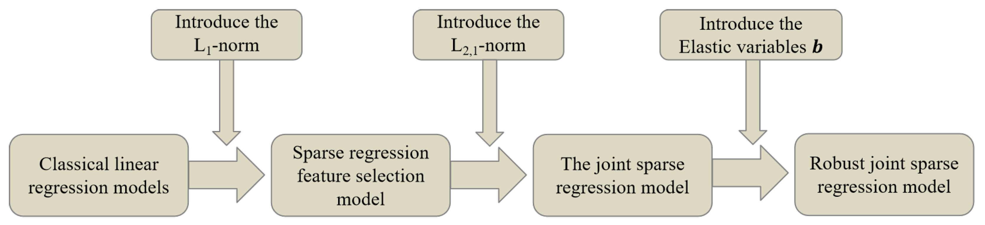
This paper proposes a robust feature selection model to overcome the traditional linear regression method’s sensitivity to noisy data and poor robustness. This paper has the following contributions: (1) The L2,1 norm is used as the regularization constraint for the projection matrix, resulting in row sparsity of the projection matrix, which eliminates irrelevant and redundant features and improves the model’s robustness to outliers. (2) To further reduce the impact of outliers, we introduce elastic variables into the loss function to supplement the fitting in the loss function and further avoid potential overfitting issues. (3) We propose a convergent and efficient robust joint sparse regression algorithm to solve the optimization problem based on the L2,1 norm objective function. (4) Through multiple experiments on three public datasets, we demonstrate the effectiveness and robustness of the model proposed in this paper. The development route of the feature selection method proposed in this paper is shown in Figure 1.

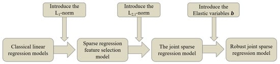
Figure 1. Development route of the feature selection methods mentioned in this paper.

2. Related Works

2.1. Related Literature

Traditional linear regression models, which learn feature coefficients through least squares, can intuitively reflect the importance of each feature in prediction and have good interpretability. However, least squares are sensitive to outliers, affecting the model’s generalization ability [25]. Ding first proposed the rotation-invariant L1 norm (R1-norm) when solving the problem of sensitivity to outliers in the sum of squared errors in the traditional principal component analysis objective function. This norm measures the distance in the space dimension using the L2 norm and sums over different data points using the L1 norm [26]. Building on this idea, Nie replaced the squared loss function in traditional linear regression models with the L2,1 norm and proposed a robust feature selection model [27]. Lai et al. proposed a generalized robust regression method using the L2,1 norm to construct loss functions and regularization terms, while also taking into account the local geometry structure of the data [28]. However, this method has a high time complexity and does not take into account the problem of data imbalance. In addition, their proposed feature extraction methods also use the L2,1 norm to improve the robustness of the model, such as rotation invariant dimensionality reduction [29] and robust local discriminant analysis [30].

Sparse regression is an approach that considers the global structure and sparsity of data in the regression algorithm. The goal is to find a sparse projection matrix that optimizes the objective function. Numerous studies have been conducted in this area by many researchers [31,32,33]. Hou et al. combined manifold learning with sparse regression, providing an innovative perspective for traditional unsupervised learning methods [34]. They also proposed a sparse matrix regression feature selection method, which uses sparse constraints on regression coefficients to select features [19]. This method has certain difficulties in the selection of sparse regularization term parameters. Chen and his colleagues utilized an in-class density map based on manifold learning as a regularizer. They created a matrix regression model using the L2,1 norm as a loss function, which they called the robust graph regularization sparse regression method [35]. However, if the image data has noise, it may be necessary to reconstruct the graph weight matrix. Additionally, adjusting parameters may also take some time. In summary, sparse regression is a widely discussed topic in the feature selection field. A summary of the relevant literature is shown in Table 1.

Table 1. A summary of relevant literature.

Type of Problem	Reference	Purpose	Method	Comment
Feature extraction	[26]	To solve the problem of principal component analysis being sensitive to outliers when minimizing the sum of squared errors.	The R1-norm is proposed and used to reconstruct the PCA objective function.	R1-PCA effectively solves the problem that loss function based on the L2 norm measure is sensitive to outliers, but the method mainly carries out robust dimensionality reduction, that is, feature extraction.
	[29]	To solve the problem that the traditional subspace learning method based on the L2 norm metric is sensitive to noise.	The L2,1 norm is used to construct the objective function.	The rotation-invariant dimension reduction algorithm has strong robustness and rotation invariance, but it has high computational complexity and is sensitive to the size of the data set.
	[30]	To solve the problem that traditional linear discriminant analysis is sensitive to noise, does not consider the local geometric structure of data, and the projection number is limited by the number of classes.	The L2,1 norm is used to construct the between-class scatter matrix and to apply joint sparsity to the projection matrix. The capped norm is used to further reduce the influence of outliers in the construction of the within-class scatter matrix.	This method is mainly used for feature extraction.
Feature selection	[27]	To solve the problem that the traditional feature selection method based on linear regression is sensitive to noise in data.	The L2,1 norm is used to construct the loss function and regularization so that the feature selection has joint sparsity.	This method is mainly used for selecting meaningful features from data in bioinformatics tasks, and there is still a potential risk of overfitting.
	[28]	To solve the problem that the number of projections in traditional ridge regression and its extension is limited by the number of categories and the robustness is poor.	The L2,1 norm constraint is applied to the loss function and regularization term to achieve joint sparsity. At the same time, the local geometric structure of the data is taken into account, and the robustness of the model is enhanced by introducing elastic factors to the loss function.	This method can perform robust image feature selection, but the computational cost is high and the case of unbalanced data is not considered.
	[34]	To solve the problem that the traditional learning-based feature selection method does not consider both manifold learning and sparse regression.	The graph weight matrix is introduced to reveal the manifold structure between data points, and the joint sparsity of feature selection is achieved by introducing the L2,1 norm regularization.	This unsupervised feature selection framework combines the advantages of manifold learning and sparse regression, but there are some open problems in the selection of parameters.
	[19]	To solve the problem of dimension disaster caused by converting two-dimensional images into one-dimensional vectors in traditional image feature selection methods.	It takes a matrix regression model to accept matrices as input and connects each matrix with its label. According to the intrinsic properties of regression coefficients, some sparsity constraints are designed for feature selection.	The regularization parameter selection of this method is complicated, but this method provides a new perspective for the study of feature selection
	[35]	To solve the problem that the feature selection method of matrix regression ignores the local geometric structure of the data.	The intra-class compactness graph based on the manifold learning is used as the regularization item, and the L2,1-norm as loss functions to establish the matrix regression model.	This method can learn both left and right regression matrices while utilizing label information to preserve its inherent geometry. However, the method has significant limitations. For instance, noise can render the graph weight matrix invalid, and the method is prone to time-consuming parameter adjustment issues.

The above sparse regression method enriches the research content in this field. By combining sparsity and regression, the selection of features is taken into account in the process of regression. The L2,1 norm is used to reduce the sensitivity of the loss function to noise and to obtain the joint sparsity of the projection matrix. However, if there is significant noise interference in the data, regression-based feature selection methods still have the potential risk of overfitting.

2.2. Linear Regression Based on Least Squares Method

Given an instance $\mathit{x}=(x_1;x_2;\dots ;x_d)\in R^{d\times 1}$ with d attributes, $x_i$ denotes the value of the i-th attribute of the instance x. A linear model tries to learn a linear combination of the attributes to achieve the prediction of the target, which can be written in vector form as

$$\mathit{f}\left(\mathit{x}\right)={\mathit{w}}^T\mathit{x}+\mathit{b}.$$

(1)

The most basic linear model can be obtained by determining w and b, where $\mathit{w}=(w_1;w_2;\dots ;w_d)\in R^{d\times 1}$ and b is a real number.

Linear regression mainly builds a loss function by measuring the error between the target value and the predicted value, so as to learn a linear model that can predict the real-valued output label as accurately as possible. Given a data set $\mathit{D}=\left\{({\mathit{x}}_1,{\mathit{y}}_1),({\mathit{x}}_2,{\mathit{y}}_2),\dots ,({\mathit{x}}_n,{\mathit{y}}_n)\right\}$, where ${\mathit{x}}_{\mathit{i}}=(x_{\mathit{i}1},x_{\mathit{i}2},\dots ,x_{\mathit{i}\mathit{d}})$, ${\mathit{y}}_{\mathit{i}}\in R$, the method of solving the model based on minimizing the mean square error is called the least squares method, and the process of solving the weight w and the bias b is called the least squares parameter estimation of linear regression, which is shown in (2):

$$({\mathit{w}}^{*},{\mathit{b}}^{*})=\underset{(\mathit{w},\mathit{b})}{min}\sum _{\mathit{i}=1}^{\mathit{n}}{(\mathit{f}\left({\mathit{x}}_i\right)-{\mathit{y}}_{\mathit{i}})}^2=\underset{(\mathit{w},\mathit{b})}{min}{∥{\mathit{w}}^T{\mathit{x}}_{\mathit{i}}+\mathit{b}-{\mathit{y}}_{\mathit{i}}∥}_2^2.$$

(2)

The goal of the least squares regression model is to minimize the error, but learning the parameters by only pursuing the unbiased estimation of the training data can easily cause overfitting, which eventually leads to a weak generalization ability of the model.

2.3. Ridge Regression, Lasso Regression, and L2,1 Norm

Traditional linear regression is prone to overfitting and has potential multicollinearity issues. Multicollinearity can lead to an increase in the variance of regression coefficients and poor model stability, making it difficult to find the true relationship between independent and dependent variables [36,37]. To address this, Arthur proposed the ridge regression model in 1970 [38], as shown in (3). Ridge regression adds a penalty term $\lambda {∥\mathit{w}∥}_2^2=\lambda {\sum }_{\mathit{i}=1}^{\mathit{d}}{\mathit{w}}_{\mathit{i}}^2$ to the least squares regression model, also known as L2 regularization.

$$\underset{(\mathit{w},\mathit{b})}{min}\sum _{\mathit{i}=1}^{\mathit{n}}{∥{\mathit{w}}^T{\mathit{x}}_{\mathit{i}}+\mathit{b}-{\mathit{y}}_{\mathit{i}}∥}_2^2+\lambda {∥\mathit{w}∥}_2^2.$$

(3)

To eliminate multicollinearity, one approach is to remove some features. Ridge regression usually only weakens multicollinearity and cannot completely eliminate it, making it unable to perform feature selection. In addition, ridge regression is sensitive to outliers and has weak robustness. Therefore, Tibshirani Robert proposed the Lasso regression model in 1996, replacing the penalty term in ridge regression with the L1 norm $\lambda {∥\mathit{w}∥}_1=\lambda {\sum }_{\mathit{i}=1}^{\mathit{d}}\left|{\mathit{w}}_{\mathit{i}}\right|$, with the optimization objective function shown in (4):

$$\underset{(\mathit{w},\mathit{b})}{min}\sum _{\mathit{i}=1}^{\mathit{n}}{∥{\mathit{w}}^T{\mathit{x}}_{\mathit{i}}+\mathit{b}-{\mathit{y}}_{\mathit{i}}∥}_2^2+\lambda {∥\mathit{w}∥}_1.$$

(4)

The L1 norm achieves feature selection by sparsifying feature coefficients, reducing the regression coefficients of some unimportant features to zero and achieving the goal of deleting some features. However, since the L1 norm is not continuously differentiable, the calculation process of Lasso regression is relatively complex. In 2006, Chris Ding first proposed the rotationally invariant L1 norm, namely the L2,1 norm, defined as shown in (5).

$${∥\mathit{W}∥}_{2,1}=\sum _{\mathit{i}=1}^{\mathit{n}}\sqrt{{\sum }_{\mathit{j}=1}^{\mathit{m}}{\mathit{w}}_{\mathit{ij}}^2}=\sum _{\mathit{i}=1}^{\mathit{n}}{∥{\mathit{w}}^{\mathit{i}}∥}_2.$$

(5)

In the matrix $\mathit{W}=\left({\mathit{w}}_{\mathit{ij}}\right)\in R^{n\times m}$, ${\mathit{w}}_{\mathit{ij}}$ is the element in the i-th row and j-th column of W, and ${\mathit{w}}^{\mathit{i}}$ is the vector composed of the elements in the i-th row of W. This norm can perform multi-task learning and tensor decomposition [39,40], and can be used as either a loss function or a regularization term [41]. When it is a loss function, because the L2 norm takes the square root of the sum of squares of the vector elements, it can reduce the model’s sensitivity to outliers and increase its robustness. When it is a regularization term, it can obtain a joint sparse projection, which can improve the performance of feature selection.

Let $\mathit{L}\left(\mathit{W}\right)={∥\mathit{W}∥}_{2,1}$. Taking the derivative of $\mathit{L}\left(\mathit{W}\right)$ with respect to W, we obtain

$$\frac{\partial \mathit{L}\left(\mathit{W}\right)}{\partial \mathit{W}}=2\mathit{DW},$$

(6)

where D is a diagonal matrix; the i-th diagonal element is

$${\mathit{D}}_{\mathit{ii}}=\frac{1}{2{∥{\mathit{w}}^{\mathit{i}}∥}_2}.$$

(7)

Hence, Equation (5) can be written as

$${∥\mathit{W}∥}_{2,1}=\mathit{Tr}\left({\mathit{W}}^T\mathit{DW}\right).$$

(8)

3. Robust Joint Sparse Regression Model

3.1. Establishment of Robust Joint Sparse Regression Model

To address the problems of traditional linear regression models, such as sensitivity to outliers, poor robustness, and weak generalization ability, this paper proposes to construct a model using robust joint sparse regression method, whose optimization objective is shown in (9):

$$\underset{(\mathit{W},\mathit{b})}{min}{∥{\mathit{X}}^T\mathit{W}+\mathbf{1}{\mathit{b}}^T-\mathit{Y}∥}_{2,1}^2+\lambda {∥\mathit{W}∥}_{2,1}.$$

(9)

This paper adopts the L2,1 norm to construct the loss objective function, where $\mathit{X}\in R^{\mathit{d}\times \mathit{n}}$ is the data matrix, $\mathit{W}\in R^{\mathit{d}\times \mathit{c}}$ is the projection matrix, an elastic variable $\mathit{b}\in R^{\mathit{c}\times 1}$ is added to the front term to alleviate the overfitting problem, the bold $\mathbf{1}\in R^{\mathit{n}\times 1}$ is a column vector of all 1s, and $\mathit{Y}\in R^{\mathit{n}\times \mathit{c}}$ is the constructed label matrix, whose elements are 0 or 1. When the i-th sample belongs to the j-th class, ${\mathit{Y}}_{\mathit{ij}}=1$; otherwise, ${\mathit{Y}}_{\mathit{ij}}=0$. The objective function consists of two terms: the front term is the residual calculation, and the back term is the L2,1 penalty term of the projection matrix W. However, the residual of this objective function is in quadratic form; therefore, it is more sensitive to outliers. In order to further improve the robustness of the model, this paper decides to adopt a non-quadratic form of loss function, whose optimization objective is shown in (10):

$$\underset{(\mathit{W},\mathit{b})}{min}{∥{\mathit{X}}^T\mathit{W}+\mathbf{1}{\mathit{b}}^T-\mathit{Y}∥}_{2,1}+\lambda {∥\mathit{W}∥}_{2,1}.$$

(10)

The elastic variable b, as a supplementary term to the loss function, aims to avoid matrix ${\mathit{X}}^T\mathit{W}$ fitting matrix Y too strictly, thereby avoiding potential overfitting problems to ensure strong generalization ability of feature selection, especially when the image is blocked by blocks or noise interference.

Compared with the traditional feature selection method based on L1 regularization, the L2,1 norm constraint can ensure the joint sparsity of W. The L2,1 norm first applies an L2 norm constraint to each row in W, forming a column vector with d elements, where each element corresponds to a feature. By applying an L1 norm constraint to this column vector, a sparse column vector is obtained, thereby achieving the joint sparsity of the projection matrix W. It is worth noting that the L2 norm is the square root of the sum of squares of each row element of the projection matrix W. This makes the elements tend to zero, so that there will be no situation where one element occupies a particularly large proportion. At this time, the features corresponding to non-zero rows of the projection matrix are selected, while the features corresponding to zero rows are discarded. $\lambda$ is a parameter that balances the front and back terms. The larger the value of $\lambda$, the higher the row sparsity of W.

3.2. The Solution of the Robust Joint Sparse Regression Model

Since there are two optimization variables, b and W, in the optimization objective (10), we first fix the projection matrix W and then solve for the elastic variable b. According to the objective function of the robust joint sparse regression model, combined with the definition of the L2,1 norm, we can obtain two diagonal matrices $\widehat{\mathit{D}}$ and $\tilde{\mathit{D}}$ from the first and second terms of Equation (10), whose diagonal elements are, respectively,

$${\widehat{\mathit{D}}}_{\mathit{ii}}=\frac{1}{2{∥{({\mathit{X}}^T\mathit{W}+\mathbf{1}{\mathit{b}}^T-\mathit{Y})}^{\mathit{i}}∥}_2},$$

(11)

$${\tilde{\mathit{D}}}_{\mathit{ii}}=\frac{1}{2{∥{\mathit{w}}^{\mathit{i}}∥}_2},$$

(12)

where ${({\mathit{X}}^T\mathit{W}+\mathbf{1}{\mathit{b}}^T-\mathit{Y})}^{\mathit{i}}$ denotes the i-th row of matrix $({\mathit{X}}^T\mathit{W}+\mathbf{1}{\mathit{b}}^T-\mathit{Y})$ and ${\mathit{w}}^{\mathit{i}}$ denotes the i-th row of matrix $\mathit{W}$; therefore, the optimization objective (10) can be written as

$$\begin{array}{cc}\hfill & \underset{(\mathit{W},\mathit{b})}{min}\mathit{Tr}\left({({\mathit{X}}^T\mathit{W}+\mathbf{1}{\mathit{b}}^T-\mathit{Y})}^T\widehat{\mathit{D}}({\mathit{X}}^T\mathit{W}+\mathbf{1}{\mathit{b}}^T-\mathit{Y})\right)+\mathit{Tr}\left({\mathit{W}}^T\tilde{\mathit{D}}\mathit{W}\right)\hfill \\ \hfill & =\underset{(\mathit{W},\mathit{b})}{min}\mathit{Tr}({\mathit{W}}^T\mathit{X}\widehat{\mathit{D}}{\mathit{X}}^T\mathit{W}+2{\mathit{W}}^T\mathit{X}\widehat{\mathit{D}}\mathbf{1}{\mathit{b}}^T-2{\mathit{W}}^T\mathit{X}\widehat{\mathit{D}}\mathit{Y}+\mathit{b}{\mathbf{1}}^T\widehat{\mathit{D}}\mathbf{1}{\mathit{b}}^T-2\mathit{b}{\mathbf{1}}^T\widehat{\mathit{D}}\mathit{Y}+{\mathit{Y}}^T\widehat{\mathit{D}}\mathit{Y})+\lambda \mathit{Tr}\left({\mathit{W}}^T\tilde{\mathit{D}}\mathit{W}\right).\hfill \end{array}$$

(13)

Next, we solve for b. Let the function $\mathit{L}(\mathit{W},\mathit{b})$ be of the following form:

$$\mathit{L}(\mathit{W},\mathit{b})=\mathit{Tr}({\mathit{W}}^T\mathit{X}\widehat{\mathit{D}}{\mathit{X}}^T\mathit{W}+2{\mathit{W}}^T\mathit{X}\widehat{\mathit{D}}\mathbf{1}{\mathit{b}}^T-2{\mathit{W}}^T\mathit{X}\widehat{\mathit{D}}\mathit{Y}+\mathit{b}{\mathbf{1}}^T\widehat{\mathit{D}}\mathbf{1}{\mathit{b}}^T-2\mathit{b}{\mathbf{1}}^T\widehat{\mathit{D}}\mathit{Y}+{\mathit{Y}}^T\widehat{\mathit{D}}\mathit{Y})+\lambda \mathit{Tr}\left({\mathit{W}}^T\tilde{\mathit{D}}\mathit{W}\right).$$

(14)

Taking the partial derivative of L(W,b) with respect to b, we obtain

$$\frac{\partial \mathit{L}(\mathit{W},\mathit{b})}{\partial \mathit{b}}=2{\mathit{W}}^T\mathit{X}\widehat{\mathit{D}}\mathbf{1}-2{\mathit{Y}}^T\widehat{\mathit{D}}\mathbf{1}+2\mathit{b}{\mathbf{1}}^T\widehat{\mathit{D}}\mathbf{1}.$$

(15)

Setting Equation (15) to zero, we can solve for b as

$$\mathit{b}=\frac{1}{{\mathbf{1}}^T\widehat{\mathit{D}}\mathbf{1}}({\mathit{Y}}^T-{\mathit{W}}^T\mathit{X})\widehat{\mathit{D}}\mathbf{1}.$$

(16)

Next, we substitute (16) into the optimization objective (10); we obtain

$$\begin{array}{cc}\hfill & \underset{\mathit{W}}{min}{∥{\mathit{X}}^T\mathit{W}+\mathbf{1}{\left(\frac{1}{{\mathbf{1}}^T\widehat{\mathit{D}}\mathbf{1}}({\mathit{Y}}^T-{\mathit{W}}^T\mathit{X})\widehat{\mathit{D}}\mathbf{1}\right)}^T-\mathit{Y}∥}_{2,1}+\lambda {∥\mathit{W}∥}_{2,1}\hfill \\ \hfill & =\underset{\mathit{W}}{min}{∥({\mathit{X}}^T-\frac{1}{{\mathbf{1}}^T\widehat{\mathit{D}}\mathbf{1}}\mathbf{1}{\mathbf{1}}^T{\widehat{\mathit{D}}}^T{\mathit{X}}^T)\mathit{W}+(\frac{1}{{\mathbf{1}}^T\widehat{\mathit{D}}\mathbf{1}}\mathbf{1}{\mathbf{1}}^T{\widehat{\mathit{D}}}^T\mathit{Y}-\mathit{Y})∥}_{2,1}+\lambda {∥\mathit{W}∥}_{2,1}\hfill \\ \hfill & =\underset{\mathit{W}}{min}\frac{1}{\lambda }{∥({\mathit{X}}^T-\frac{1}{{\mathbf{1}}^T\widehat{\mathit{D}}\mathbf{1}}\mathbf{1}{\mathbf{1}}^T{\widehat{\mathit{D}}}^T{\mathit{X}}^T)\mathit{W}+(\frac{1}{{\mathbf{1}}^T\widehat{\mathit{D}}\mathbf{1}}\mathbf{1}{\mathbf{1}}^T{\widehat{\mathit{D}}}^T\mathit{Y}-\mathit{Y})∥}_{2,1}+{∥\mathit{W}∥}_{2,1}.\hfill \end{array}$$

(17)

At this point, we need to simplify the optimization objective and then solve for W using the method provided in reference [27]. First, we let $({\mathit{X}}^T-\frac{1}{{\mathbf{1}}^T\widehat{\mathit{D}}\mathbf{1}}\mathbf{1}{\mathbf{1}}^T{\widehat{\mathit{D}}}^T{\mathit{X}}^T)\mathit{W}+(\frac{1}{{\mathbf{1}}^T\widehat{\mathit{D}}\mathbf{1}}\mathbf{1}{\mathbf{1}}^T{\widehat{\mathit{D}}}^T\mathit{Y}-\mathit{Y})=\mathit{Q}$, resulting in the following optimization objective:

$$\begin{array}{c}\hfill \underset{\mathit{W}}{min}{∥\mathit{Q}∥}_{2,1}+{∥\mathit{W}∥}_{2,1}s.t.(\mathit{I}-\frac{1}{{\mathbf{1}}^T\widehat{\mathbf{D}}\mathbf{1}}\mathbf{1}{\mathbf{1}}^T{\widehat{\mathbf{D}}}^T){\mathit{X}}^T\mathit{W}+\lambda \mathit{Q}=\mathit{Y}-\frac{1}{{\mathbf{1}}^T\widehat{\mathbf{D}}\mathbf{1}}\mathbf{1}{\mathbf{1}}^T{\widehat{\mathbf{D}}}^T\mathit{Y}.\end{array}$$

(18)

At this point, we use the following formula to calculate Q:

$$\mathit{Q}=\frac{1}{\lambda }(\mathit{I}-\frac{1}{{\mathbf{1}}^T\widehat{\mathbf{D}}\mathbf{1}}\mathbf{1}{\mathbf{1}}^T{\widehat{\mathbf{D}}}^T)(\mathit{Y}-{\mathit{X}}^T\mathit{W}).$$

(19)

We write (18) in the following form:

$$\underset{\mathit{W}}{min}{∥\left[\begin{array}{c}\mathit{W}\\ \mathit{Q}\end{array}\right]∥}_{2,1}s.t.\left[\begin{array}{cc}(\mathit{I}-\frac{1}{{\mathbf{1}}^T\widehat{\mathbf{D}}\mathbf{1}}\mathbf{1}{\mathbf{1}}^T{\widehat{\mathbf{D}}}^T){\mathit{X}}^T,& \lambda \mathit{I}\end{array}\right]\left[\begin{array}{c}\mathit{W}\\ \mathit{Q}\end{array}\right]=\mathit{Y}-\frac{1}{{\mathbf{1}}^T\widehat{\mathbf{D}}\mathbf{1}}\mathbf{1}{\mathbf{1}}^T{\widehat{\mathbf{D}}}^T\mathit{Y},$$

(20)

where I is the identity matrix. We let the matrices P, M, N be equal to the following formulas:

$$\mathit{P}=\left[\begin{array}{c}\mathit{W}\\ \mathit{Q}\end{array}\right],$$

(21)

$$\mathit{M}=\left[\begin{array}{cc}(\mathit{I}-\frac{1}{{\mathbf{1}}^T\widehat{\mathbf{D}}\mathbf{1}}\mathbf{1}{\mathbf{1}}^T{\widehat{\mathbf{D}}}^T){\mathit{X}}^T,& \lambda \mathit{I}\end{array}\right],$$

(22)

$$\mathit{N}=\mathit{Y}-\frac{1}{{\mathbf{1}}^T\widehat{\mathbf{D}}\mathbf{1}}\mathbf{1}{\mathbf{1}}^T{\widehat{\mathbf{D}}}^T\mathit{Y}.$$

(23)

Then, (20) can be written as the following form, which leads to the final optimization objective:

$$\underset{\mathit{P}}{min}{∥\mathit{P}∥}_{2,1}s.t.\mathit{MP}=\mathit{N}.$$

(24)

Since the L2,1 norm is convex, we can use the Lagrange multiplier method to solve the optimization objective (24), as shown below:

$$\mathit{L}\left(\mathit{P}\right)={∥\mathit{P}∥}_{2,1}-\mathit{Tr}\left({\Lambda }^T(\mathit{MP}-\mathit{N})\right).$$

(25)

Taking the derivative of L(P) with respect to P and then setting it to zero, we have

$$\frac{\partial \mathit{L}\left(\mathit{P}\right)}{\partial \mathit{P}}=2\mathit{DP}-{\mathit{M}}^T\mathsf{\Lambda }=0.$$

(26)

By the property of the L2,1 norm, D is a diagonal matrix, whose i-th diagonal element is

$${\mathit{D}}_{\mathit{ii}}=\frac{1}{2{∥{\mathit{p}}^{\mathit{i}}∥}_2},$$

(27)

where ${\mathit{p}}^{\mathit{i}}$ denotes the i-th row of matrix P. Rearranging Equation (26), we have

$$\begin{array}{cc}\hfill & 2\mathit{P}={\mathit{D}}^{-1}{\mathit{M}}^T\mathsf{\Lambda },\hfill \\ \hfill & \Rightarrow 2\mathit{MP}=\mathit{M}{\mathit{D}}^{-1}{\mathit{M}}^T\mathsf{\Lambda }.\hfill \end{array}$$

(28)

Substituting the constraint from Equation (24) into Equation (28), we obtain

$$\begin{array}{cc}\hfill & 2\mathit{N}=\mathit{M}{\mathit{D}}^{-1}{\mathit{M}}^T\mathsf{\Lambda },\hfill \\ \hfill & \Rightarrow \mathsf{\Lambda }=2{\left(\mathit{M}{\mathit{D}}^{-1}{\mathit{M}}^T\right)}^{-1}\mathit{N}.\hfill \end{array}$$

(29)

Then, substituting Equation (29) into Equation (28), we obtain

$$\mathit{P}={\mathit{D}}^{-1}{\mathit{M}}^T{\left(\mathit{M}{\mathit{D}}^{-1}{\mathit{M}}^T\right)}^{-1}\mathit{N}.$$

(30)

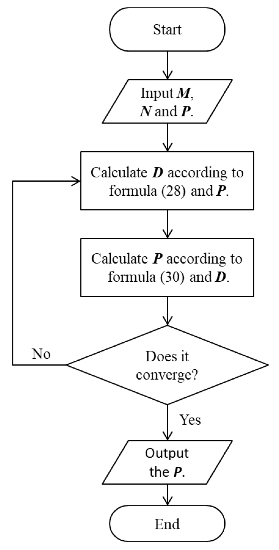
From Equation (27), we know that D depends on the value of P, and, from Equation (30), we know that the value of P is related to the value of D. According to the definition of the matrix P (20), we can obtain the projection of matrix W through P. Therefore, we can use an iterative process to solve this problem, and the detailed algorithm steps are shown in Algorithm 1 and Figure 2.

Algorithm 1: Iterative process of solving matrix P

Input: Data M, N, and P

Output: P matrix

1: Use the latest P to calculate D according to Equation (27);

2: Use the latest D to update P according to Equation (30);

3: Repeat steps 1 and 2 until convergence;

4: Output the current P.

Figure 2. Flow chart of Algorithm 1.

Considering that there are two iterative processes in the whole solution process of the robust joint sparse regression model, we design the robust joint sparse regression algorithm, as shown in Algorithm 2 and Figure 3.

Algorithm 2: Robust Joint Sparse Regression Algorithm

Input: Training data $\mathit{X}\in R^{\mathit{d}\times \mathit{n}}$, labels $\mathit{Y}\in R^{\mathit{n}\times \mathit{c}}$, parameter $\lambda$

Output: Projection matrix $\mathit{W}\in R^{\mathit{d}\times \mathit{c}}$ and elastic variable $\mathit{b}\in R^{1\times \mathit{c}}$

1: Randomly initialize W and b;

2: Calculate the diagonal matrix $\widehat{\mathit{D}}$ according to Equation (11);

3: Use the values of $\widehat{\mathit{D}}$, X, Y, and W to update Q according to Equation (19);

4: Use the values of $\widehat{\mathit{D}}$, X, and $\lambda$ to update M according to Equation (22);

5: Use the values of $\widehat{\mathit{D}}$ and Y to update N according to Equation (23);

6: Use the values of W and Q to calculate P according to Equation (21);

7: Use the values of P, M, and N to update P according to Algorithm 1;

8: Update W with the latest P;

9: Update b with the latest W;

10: Repeat steps 2 to 9 until convergence.

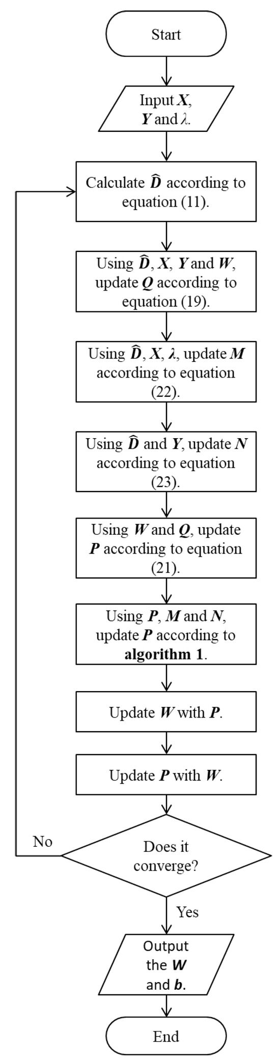
Figure 3. Flow chart of Algorithm 2.

4. Results

In order to assess the effectiveness of our proposed model, we conducted several experiments using three different datasets. Our comparison included 10 different algorithms: Sparse Principal Component Analysis (SPCA) [42], Kernel Principal Component Analysis (KPCA) [43], Locality-Preserving Projections (LPP) [44], Ridge Regression (RR), Laplacian Score (LS) [45], L1 regularization methods (including the Least absolute shrinkage and selection operator (LASSO)), Multi-Cluster Feature Selection (MCFS) [46], and Elastic Net (ElasticNet), as well as L2,1 regularization methods such as Joint Embedding Learning and Sparse Regression (JELSR) [34] and Unsupervised Discriminative Feature Selection (UDFS) [41].

To evaluate the performance of our feature selection model, we measure the classification accuracy of the k-nearest neighbor (KNN) classifier [47]. We use the chosen features as input for the classifier and set the k value to 1 in all our experiments. As computational resources are limited, we apply principal component analysis (PCA) to preprocess the original data and reduce its dimensionality before each experiment. We update the parameters of our feature selection model on the training set, fine-tune the hyperparameters on the validation set, and compare it with other algorithms on the test set. We conduct five separate tests and report the average results as the final evaluation of our model.

4.1. Experiments on the JAFFE Dataset

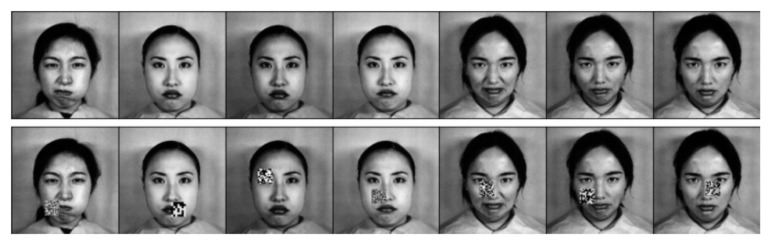
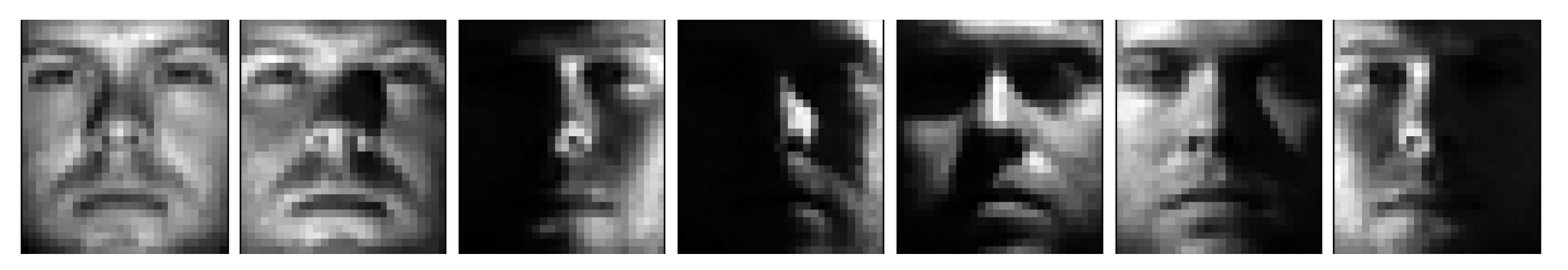
The JAFFE dataset, which was developed by Michael Lyons, Miyuki Kamachi, and Jiro Gyoba [48], consists of 213 photographs featuring 10 Japanese female models displaying seven facial expressions each. These expressions include one neutral expression and six basic expressions. Each image was rated by 60 volunteers based on six emotional adjectives. The resolution of each image is 256 × 256 pixels. Figure 4 provides some examples of the images included in the dataset.

Figure 4. Examples of different facial expression images from the JAFFE dataset.

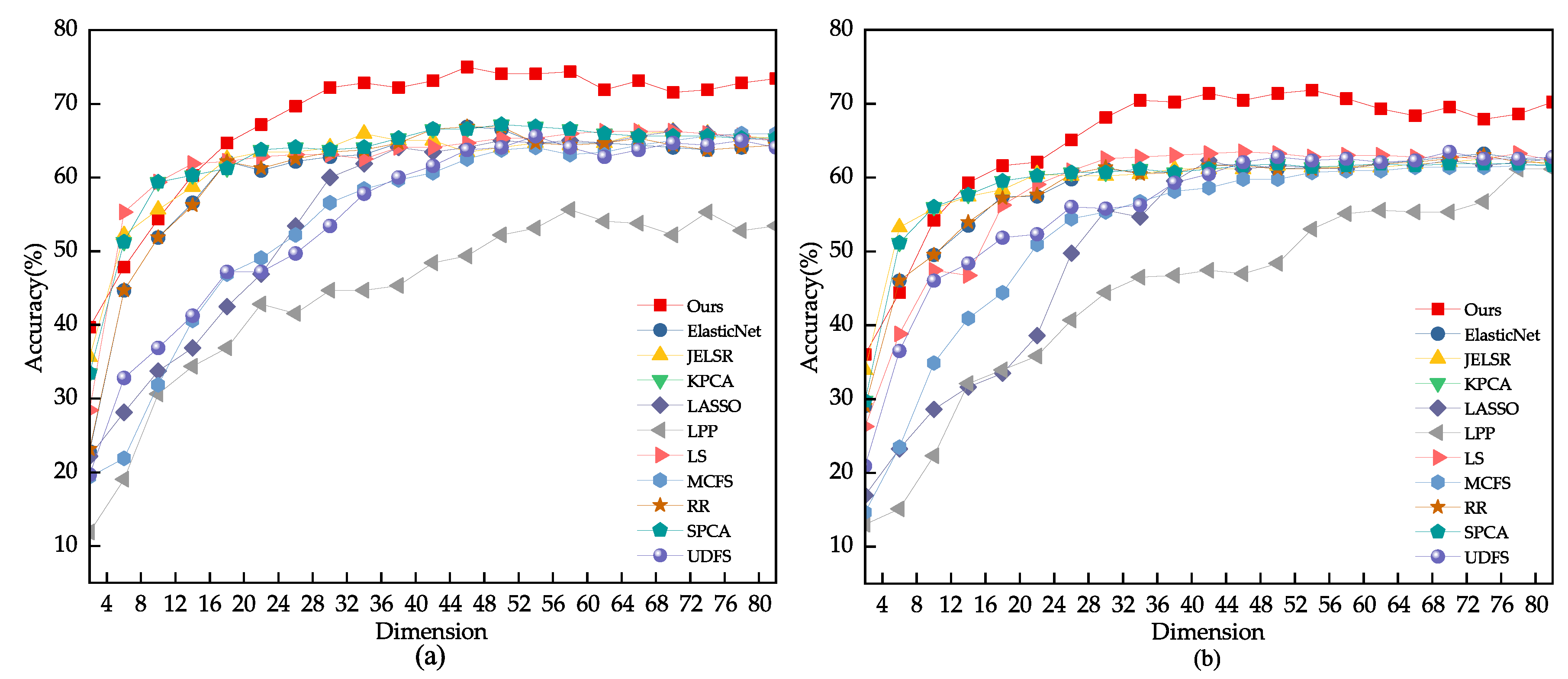
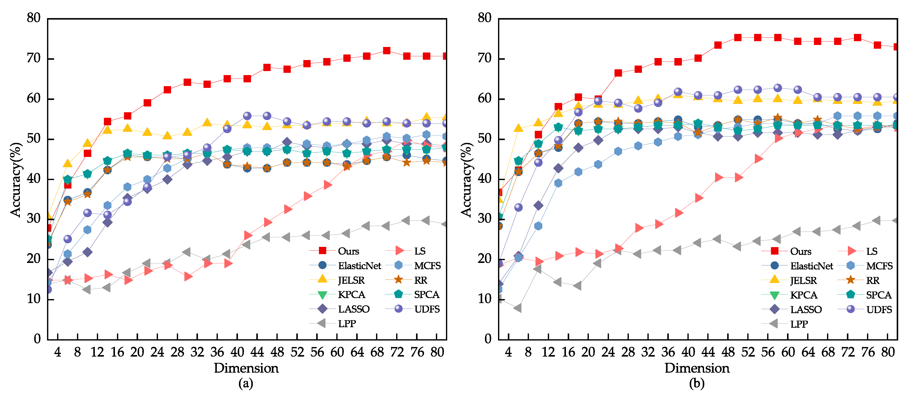
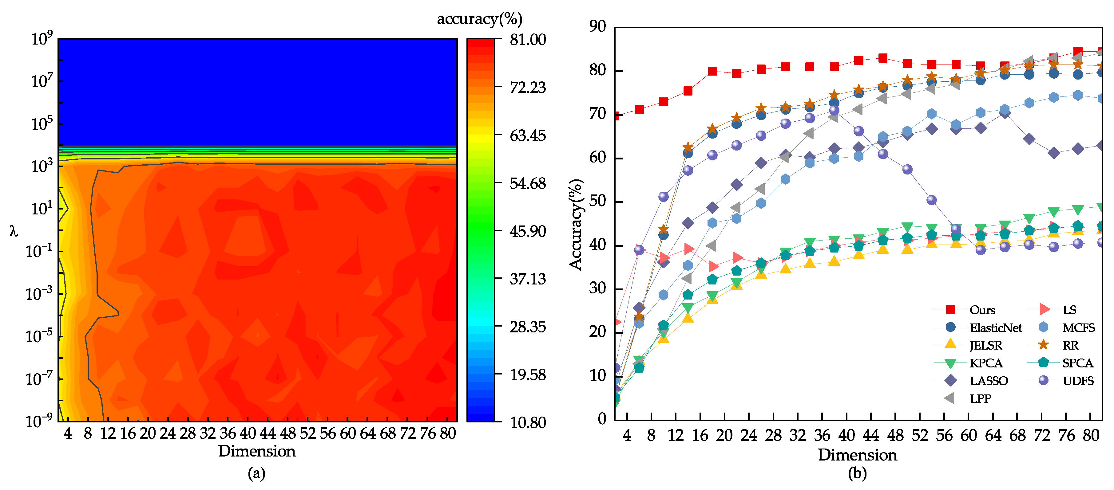
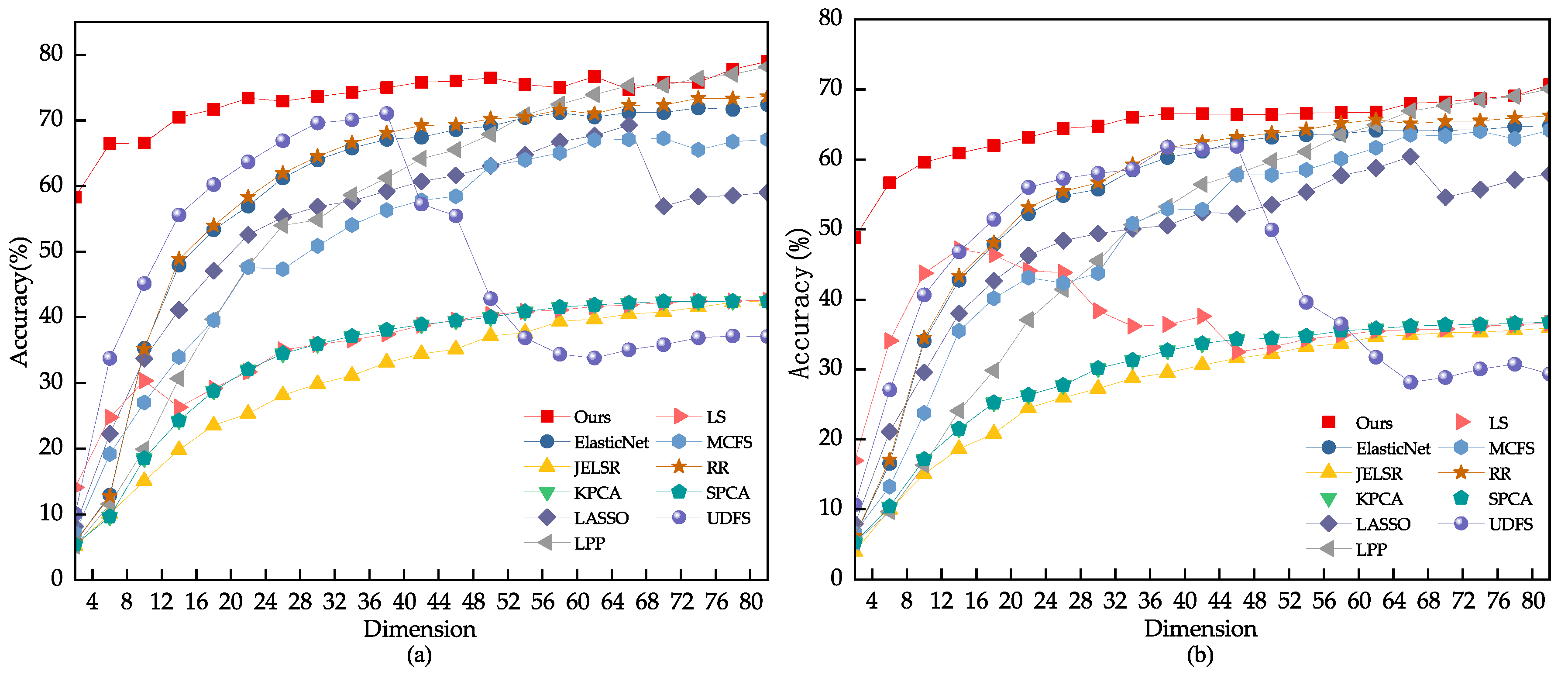
We conducted a grid search on the dataset to find the best range for the model parameter $\lambda$. For other comparison algorithms, we referred to the settings in their original papers, such as using $[{10}^{-3},{10}^3]$ for UDFS. We split the images from each class into 40%, 50%, and 60% for training. Based on Figure 5, the optimal range we found for the $\lambda$ parameter through grid search is $[{10}^{-8},{10}^{-3}]$. Figure 5 and Figure 6 present the comparison results of various feature selection methods under different dataset splits. Table 2 provides the average accuracy, standard deviation, and feature count of different models on the JAFFE dataset. From the experimental data, it is evident that the feature subset selected by our model performs better than other algorithms on the JAFFE dataset.

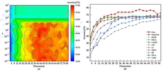
Figure 5. (a) The classification outcome corresponding to the variation of $\lambda$ on the JAFFE dataset. (b) Using 80% of the samples randomly drawn from the JAFFE dataset as the training set.

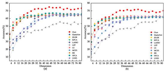
Figure 6. (a) Using 60% of the samples randomly drawn from the JAFFE dataset as the training set. (b) Using 40% of the samples randomly drawn from the JAFFE dataset as the training set.

Table 2. The corresponding accuracy, standard deviation, and feature number of different algorithms on the JAFFE dataset.

Training Sample (%)	Ours	LASSO	LS	SPCA	JELSR	UDFS	LPP	ElasticNet	KPCA	RR	MCFS
40%	71.86 ± 3.89 54	62.56 ± 6.34 82	63.49 ± 3.35 46	61.86 ± 6.55 50	62.56 ± 6.34 74	62.79 ± 7.07 50	61.16 ± 4.62 78	63.26 ± 1.56 74	61.86 ± 6.55 50	63.02 ± 1.91 74	61.40 ± 5.03 66
60%	74.06 ± 3.92 50	66.25 ± 2.84 70	66.25 ± 3.60 62	67.19 ± 3.66 50	66.25 ± 5.25 70	65.63 ± 4.56 54	55.63 ± 7.46 58	66.88 ± 5.11 46	67.19 ± 3.66 50	66.56 ± 5.01 42	65.94 ± 6.85 78
80%	77.67 ± 3.89 58	69.30 ± 5.55 70	67.91 ± 7.05 62	68.37 ± 7.09 50	69.30 ± 7.78 74	68.37 ± 5.84 66	63.72 ± 5.84 82	68.37 ± 4.23 50	68.37 ± 7.09 50	68.37 ± 4.23 50	68.37 ± 2.65 82

Note: The first number in the cell represents accuracy, the second number represents standard deviation, and the third number represents the number of features.

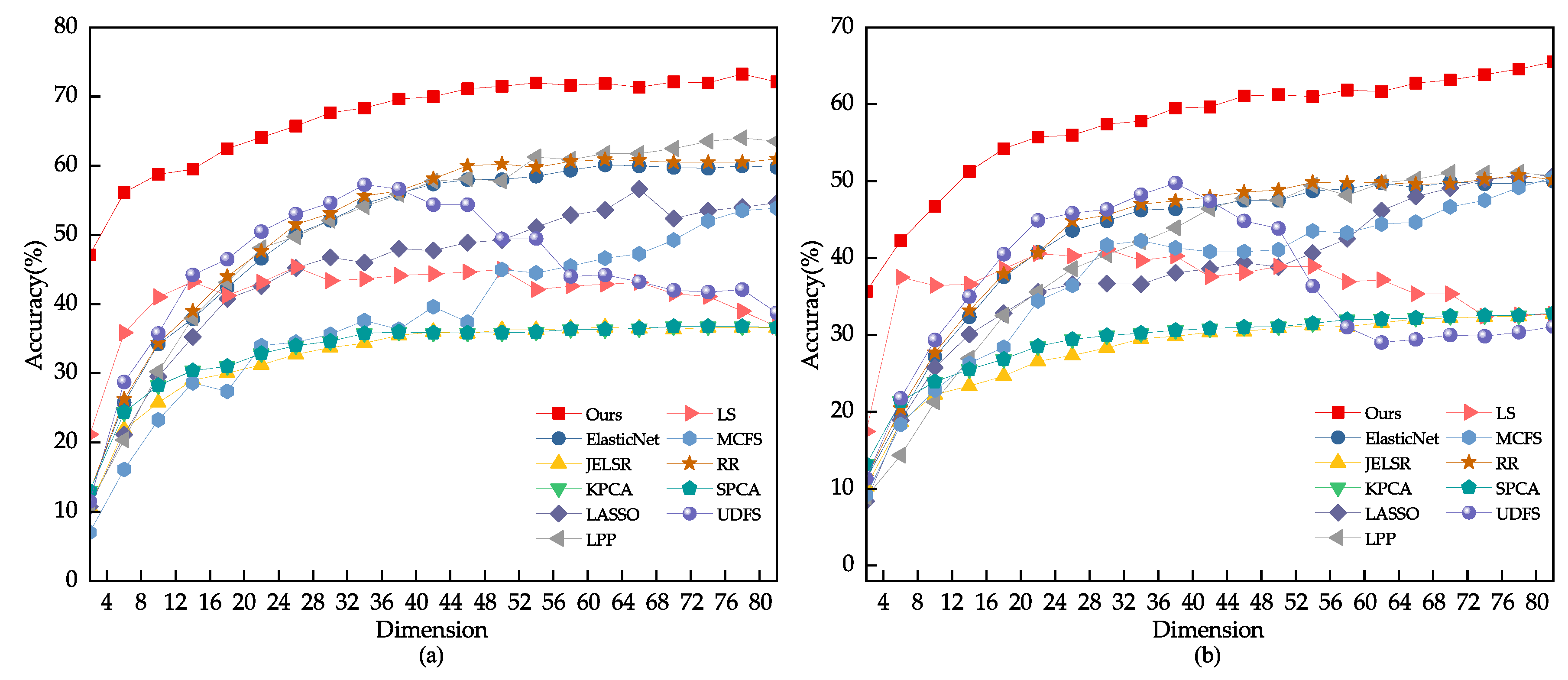
Due to the inherent challenge posed by environmental variations in the face images randomly extracted from the CMU PIE and YALEB datasets for feature selection tasks, this study chose to conduct an expansion experiment on the JAFFE dataset. The test set for this experiment consisted of 20% of the dataset, with 80% being used as the training and validation set. Block noise of sizes 15 × 15, 25 × 25, and 35 × 35 pixels were randomly applied to the face images in the test set. The results of the experiment are illustrated in Figure 7 and Figure 8, with detailed data presented in Table 3. The comparison results indicate that other feature selection methods were significantly affected by the noise, resulting in decreased discriminative ability of the selected feature subset. Locality-Preserving Projection (LPP) and Laplacian Score (LS) were particularly sensitive to noise, as their performance showed a significant decrease. In contrast, the proposed model presented in this study exhibited stability and was less sensitive to noise.

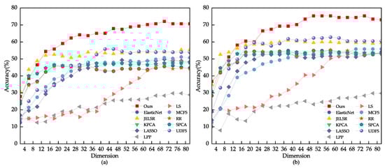
Figure 7. (a) Feature selection performance of different algorithms when adding block noise of size 15 × 15 pixels to JAFFE test images. (b) Feature selection performance of different algorithms when adding block noise of size 25 × 25 pixels to JAFFE test images.

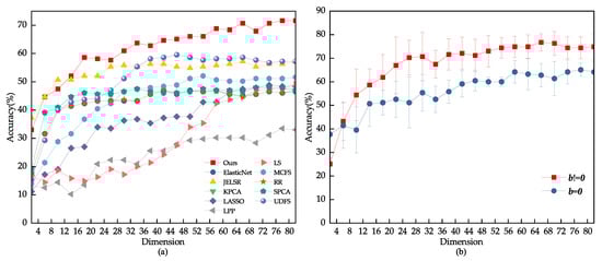
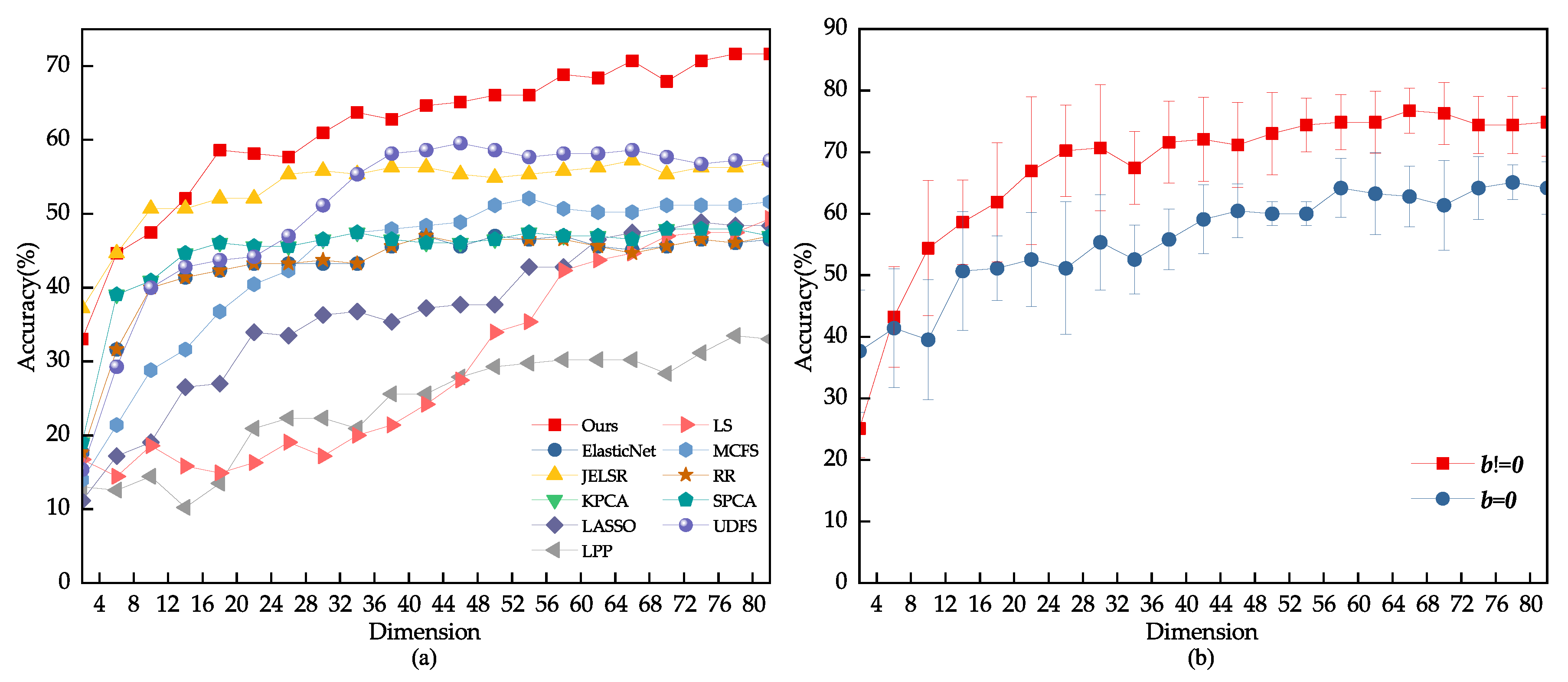
Figure 8. (a) Feature selection performance of different algorithms when adding block noise of size 35 × 35 pixels to JAFFE test images. (b) Ablation experiment of elastic variables when adding block noise of size 35 × 35 pixels to JAFFE test images.

Table 3. Comparison of feature selection performance of different algorithms when adding block noise of different sizes.

Block Size	Ours	LASSO	LS	SPCA	JELSR	UDFS	LPP	ElasticNet	KPCA	RR	MCFS
$15\times 15$	72.09 ± 3.68 70	49.30 ± 1.95 50	49.77 ± 4.82 74	47.91 ± 4.82 82	55.35 ± 8.29 78	55.81 ± 9.59 42	29.77 ± 16.39 74	46.05 ± 5.04 74	47.91 ± 4.82 82	46.51 ± 2.85 34	51.16 ± 1.64 78
$25\times 25$	75.35 ± 5.35 50	53.02 ± 12.57 38	53.49 ± 10.00 78	53.95 ± 9.21 42	60.93 ± 9.21 38	62.79 ± 10.90 58	29.77 ± 18.12 78	54.88 ± 8.32 38	53.95 ± 9.21 42	55.35 ± 7.05 58	55.81 ± 9.73 70
$35\times 35$	71.63 ± 1.95 78	43.84 ± 7.89 74	50.00 ± 6.45 82	47.90 ± 8.16 70	57.21 ± 6.90 66	58.61 ± 7.24 50	33.49 ± 14.20 78	46.98 ± 4.16 42	47.91 ± 8.16 70	46.98 ± 4.47 82	51.63 ± 6.66 82

Note: The first number in the cell represents accuracy, the second number represents standard deviation, and the third number represents the number of features.

To verify the role of elastic variables in the fitting process of the loss function, this paper conducted an ablation experiment of elastic variables on the JAFFE dataset. The dataset was split into a 60% training set and a 40% test set, with block noise of 35 × 35 pixels added to the test set. Five independent experiments were conducted, and the average result was used to evaluate the elastic variables. Figure 8 shows the experimental results. The results suggest that, when an image contains random block noise, the elastic variable b, as a supplementary term in the loss function, helps to prevent overfitting. Consequently, the model exhibits greater robustness to noise.

4.2. Experiments on the CMU PIE Dataset

The CMU PIE dataset [49] was established in 2000 and contains 40,000 facial images of 68 people captured in different poses, lighting, and expressions. In our study, we randomly chose 400 face images of 20 people from the dataset and resized them to 32 × 32 pixels. Some of the chosen face images are shown in Figure 9.

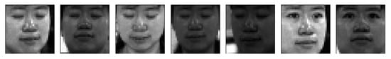
Figure 9. Examples of face images with different poses and illuminations from the CMU PIE dataset.

The dataset was split into two sets for training and testing. The training sets consisted of 40%, 60%, and 80% of the images, while the remainder were used for testing. To determine the most suitable $\lambda$ parameter range, a grid search was conducted, and the optimal value was found to be $[{10}^{-9},{10}^2]$, as shown in Figure 10. The outcomes of various feature selection techniques on the PIE dataset are displayed in Figure 10 and Figure 11, with Table 4 presenting the average recognition rate, standard deviation, and number of features for different methods in the face recognition test. The results indicate that the UDFS model experiences a significant decrease when the number of features is between 30 and 80 due to the selection of some interfering features. In contrast, the robust joint sparse regression model proposed in this study can select more discriminative features, even with pose and illumination variations in face images, resulting in an overall upward trend.

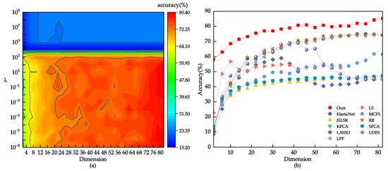
Figure 10. (a) The classification outcome corresponding to the variation of $\lambda$ on the CMU PIE dataset. (b) Using 80% of the samples randomly drawn from the CMU PIE dataset as the training set.

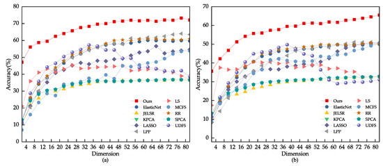
Figure 11. (a) Using 60% of the samples randomly drawn from the CMU PIE dataset as the training set. (b) Using 40% of the samples randomly drawn from the CMU PIE dataset as the training set.

Table 4. The corresponding accuracy, standard deviation, and feature number of different algorithms on the CMU PIE dataset.

Training Sample (%)	Ours	LASSO	LS	SPCA	JELSR	UDFS	LPP	ElasticNet	KPCA	RR	MCFS
40%	65.50 ± 4.44 82	50.75 ± 9.54 82	41.17 ± 4.40 30	32.83 ± 3.60 82	32.75 ± 4.02 82	49.75 ± 2.22 38	51.08 ± 4.69 70	50.00 ± 4.44 82	32.83 ± 3.60 82	50.75 ± 3.83 78	50.50 ± 8.16 82
60%	73.25 ± 4.41 78	56.63 ± 11.38 66	65.38 ± 2.28 26	36.75 ± 2.14 70	36.63 ± 2.92 62	57.25 ± 4.16 34	64.00 ± 2.85 78	60.13 ± 3.84 62	36.75 ± 2.14 70	61.00 ± 3.96 82	53.88 ± 9.43 82
80%	85.25 ± 2.40 82	59.00 ± 11.16 34	54.75 ± 4.28 34	47.00 ± 4.81 82	46.50 ± 4.45 78	69.00 ± 10.58 42	74.75 ± 4.87 82	75.00 ± 3.19 70	47.00 ± 4.81 82	74.50 ± 4.20 78	61.75 ± 6.71 78

Note: The first number in the cell represents accuracy, the second number represents standard deviation, and the third number represents the number of features.

4.3. Experiments on the YaleB Dataset

The YaleB database had 2432 face images from 38 different subjects [50]. Each subject had around 64 near-frontal pictures taken under different lighting conditions. The images were cropped and resized to 32 × 28 pixels. Some of the chosen face images are displayed in Figure 12.

Figure 12. Examples of face images in the YaleB dataset under different lighting, expression, and glasses conditions.

We conducted a grid search on the YaleB dataset and found that the optimal parameter range is $[{10}^{-6},{10}^3]$. As shown in Figure 13 and Figure 14, we compared the performance of different algorithms for feature selection on the YaleB dataset. Table 5 shows the results of the face recognition experiment, including the average recognition rate, standard deviation, and number of features for different methods. Our proposed method outperforms Locality-Preserving Projection (LPP), Ridge Regression (RR), and ElasticNet methods in terms of feature subset selection. However, it is worth noting that the UDFS method shows a significant decline when around 40 features are selected. This is because the UDFS method chooses some interfering features that affect the discriminability of the feature subset.

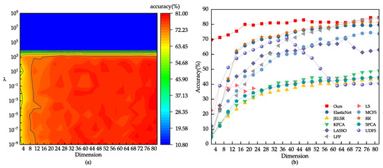
Figure 13. (a) The classification outcome corresponding to the variation of $\lambda$ on the YaleB dataset. (b) Using 80% of the samples randomly drawn from the YaleB dataset as the training set.

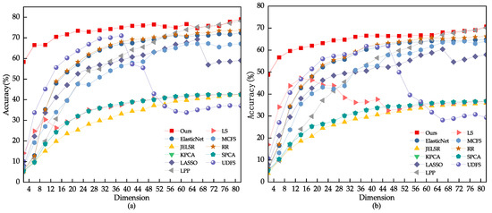
Figure 14. (a) Using 60% of the samples randomly drawn from the YaleB dataset as the training set. (b) Using 40% of the samples randomly drawn from the YaleB dataset as the training set.

Table 5. The corresponding accuracy, standard deviation, and feature number of different algorithms on the YaleB dataset.

Training Sample (%)	Ours	LASSO	LS	SPCA	JELSR	UDFS	LPP	ElasticNet	KPCA	RR	MCFS
40%	70.67 ± 4.81 82	60.42 ± 14.68 66	47.17 ± 11.30 14	36.75 ± 3.67 82	35.91 ± 4.27 82	61.42 ± 8.29 42	70.08 ± 5.45 82	64.83 ± 1.99 82	36.75 ± 3.67 82	66.25 ± 1.02 82	64.17 ± 6.99 82
60%	79.00 ± 5.60 82	67.67 ± 17.18 62	42.63 ± 6.49 82	42.50 ± 6.43 78	42.54 ± 6.70 82	71.04 ± 5.14 38	78.17 ± 3.64 82	72.42 ± 3.35 82	42.50 ± 6.43 78	73.67 ± 2.62 82	67.25 ± 7.31 70
80%	84.50 ± 3.38 78	70.50 ± 16.29 66	44.25 ± 6.59 74	44.50 ± 6.94 78	43.50 ± 7.09 82	71.00 ± 5.41 38	84.25 ± 3.26 82	79.75 ± 3.79 82	49.00 ± 5.48 82	81.50 ± 2.56 74	74.50 ± 1.68 78

Note: The first number in the cell represents accuracy, the second number represents standard deviation, and the third number represents the number of features.

4.4. Convergence Analysis

The robust joint sparse regression algorithm involves two iterative processes, and two conditions control the iteration stops. The first condition is a fixed number of iterations, which is generally set to 500 times, and the second condition is the convergence of the value of the objective function. From this, 80% of the samples are selected as training and validation sets, and examples of iterative convergence on three datasets are given. As shown in Figure 15, the algorithm proposed in this paper has a fast convergence speed.

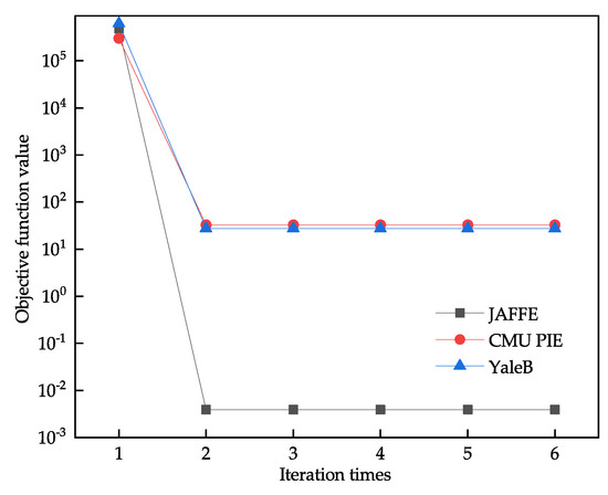
Figure 15. Examples of iterative convergence of the algorithm on three datasets.

5. Discussion

Traditional feature selection methods based on linear regression and regularization methods are simple to use and have strong interpretability, but are easily affected by outliers. When there is a high degree of correlation among features in the data, these traditional linear regression-based feature selection methods struggle to effectively distinguish the importance of correlated features. To address these challenges, this paper proposes a robust joint sparse regression feature selection method.

In this study, we conducted a thorough validation of our model by conducting a series of experiments. Firstly, we tested the model’s capability to select features for various facial expression recognition tasks using the JAFFE dataset. We then evaluated its robustness in handling outliers when block noise is introduced. Our model uses an L2,1 norm-based loss function that is insensitive to outliers, which enables it to select effective subsets of features even after block noise is added to facial images. We conducted ablation experiments with elastic variables and confirmed that, when the number of training samples is fewer than the number of test samples, elastic variables can effectively prevent overfitting. In contrast, other feature selection methods are significantly affected by noise.

We assessed our model’s capability to pick out features from two sets of facial images with different poses, lighting, and expressions. Our model uses L2,1 norm-based regularization to implement structured sparse regularization, which takes into account the connections between features and selects them through shared sparsity across all categories. This strategy effectively decreases data redundancy and noise while enhancing model generalization and computational efficiency. Lastly, we analyzed how well our proposed algorithm performs in terms of convergence.

To summarize, the paper proposes a model that efficiently picks out significant features for a given task and eliminates unnecessary ones. The model also shows strong robustness by remaining unaffected by any noise or outliers found in the dataset. In upcoming research, we may explore extending the L2,1 norm to the L2,p norm to conduct further studies and develop novel models.

6. Conclusions

In this paper, we propose a robust joint L2,1 norm minimization sparse regression feature selection method, which solves the problem of poor robustness existing in traditional linear regression feature selection methods. The loss function based on the L2,1 norm is less sensitive to outliers than the loss function based on the L2 norm metric, and the regularization based on the L2,1 norm can make the feature selection have joint sparsity compared with the L1 norm regularization. By providing a supplement for the fitting of the loss function, the elastic variable effectively prevents the problem of poor robustness of the model caused by overfitting in the face of noisy data, making the model more robust. We have designed two iterative processes and proposed an efficient and convergent robust joint sparse regression algorithm to implement the model. Our experiments on three typical datasets have shown that our model’s feature selection ability is superior to traditional Ridge Regression (RR), Sparse Principal Component Analysis (SPCA), Locally Preserving Projection (LPP), and Laplacian Score (LS), as well as methods based on L1 regularization such as Lasso, MCFS, and ElasticNet. Additionally, it outperforms methods based on L2,1 regularization such as UDFS and JELSR.

References

- Ding, C.; Peng, H. Minimum redundancy feature selection from microarray gene expression data. J. Bioinform. Comput. Biol. 2005, 2, 185–205. [Google Scholar] [CrossRef] [PubMed]
- Beatriz, R.; Verónica, B. A review of feature selection methods in medical applications. Comput. Biol. Med. 2019, 122, 103375. [Google Scholar]
- Last, M.; Kandel, A.; Maimon, O. Information-theoretic algorithm for feature selection. Pattern Recognit. Lett. 2001, 22, 799–811. [Google Scholar] [CrossRef]
- Koller, D.; Sahami, M. Toward Optimal Feature Selection. In Proceedings of the 13th International Conference on Machine Learning, Bari, Italy, 3–6 July 1996; Volume 9, pp. 284–292. [Google Scholar]
- Kira, K.; Rendell, L.A. A practical approach to feature selection. In Machine Learning Proceedings 1992; Sleeman, D., Edwards, P., Eds.; Morgan Kaufmann: San Mateo, CA, USA, 1992; pp. 249–256. [Google Scholar]
- Avrim, L.B.; Pat, W.L. Selection of relevant features and examples in machine learning. Artif. Intell. 1997, 97, 245–271. [Google Scholar]
- Khaire, U.M.; Dhanalakshmi, R. Stability of feature selection algorithm: A review. J. King Saud Univ.—Comput. Inf. Sci. 2022, 34, 1060–1073. [Google Scholar]
- Gongmin, L.; Chenping, H.; Feiping, N.; Tingjin, L.; Dongyun, Y. Robust feature selection via simultaneous sapped norm and sparse regularizer minimization. Neurocomputing 2018, 283, 228–240. [Google Scholar]
- Dash, M.; Choi, K.; Scheuermann, P.; Liu, H. Feature Selection for Clustering—A Filter Solution. In Proceedings of the 2002 IEEE International Conference on Data Mining, Maebashi City, Japan, 9–12 December 2002; pp. 115–122. [Google Scholar]
- Huang, Q.; Tao, D.; Li, X.; Jin, L.; Wei, G. Exploiting Local Coherent Patterns for Unsupervised Feature Ranking. IEEE Trans. Syst. Man Cybern. 2011, 41, 1471–1482. [Google Scholar] [CrossRef] [PubMed]
- Kohavi, R.; John, G.H. Wrappers for Feature Subset Selection. Artif. Intell. 1997, 97, 273–324. [Google Scholar] [CrossRef]
- Guyon, I.; Elisseeff, A. An Introduction to Variable and Feature Selection. J. Mach. Learn. Res. 2003, 3, 1157–1182. [Google Scholar]
- Hou, C.; Nie, F.; Yi, D.; Wu, Y. Feature Selection via Joint Embedding Learning and Sparse Regression. In Proceedings of the International Joint Conference on Artificial Intelligence, Barcelona, Spain, 16–22 July 2011; pp. 1324–1329. [Google Scholar]
- Zhao, Z.; Wang, L.; Liu, H. Efficient Spectral Feature Selection with Minimum Redundancy. In Proceedings of the AAAI Conference on Artificial Intelligence, Atlanta, GA, USA, 11–15 July 2010; pp. 673–678. [Google Scholar]
- Meng, L. Embedded feature selection accounting for unknown data heterogeneity. Expert Syst. Appl. 2019, 119, 350–361. [Google Scholar]
- Tibshirani, R. Regression Shrinkage and Selection via the Lasso. J. R. Stat. Soc. B 1996, 58, 267–288. [Google Scholar] [CrossRef]
- Donoho, D.L. For most large underdetermined systems of linear equations the minimal L1-norm solution is also the sparsest solution. Commun. Pure Appl. Math. 2006, 59, 797–829. [Google Scholar] [CrossRef]
- Hui, Z.; Trevor, H. Regularization and variable selection via the elastic net. J. R. Stat. Soc. B 2005, 67, 301–320. [Google Scholar]
- Hou, C.; Jiao, Y.; Nie, F.; Luo, T.; Zhou, Z.H. 2D Feature Selection by Sparse Matrix Regression. IEEE Trans. Image Process. 2017, 26, 4255–4268. [Google Scholar] [CrossRef] [PubMed]
- Mo, D.; Lai, Z. Robust Jointly Sparse Regression with Generalized Orthogonal Learning for Image Feature Selection. Pattern Recognit. 2019, 93, 164–178. [Google Scholar] [CrossRef]
- Lemhadri, I.; Tibshirani, R.; Hastie, T. LassoNet: A neural network with feature sparsity. J. Mach. Learn. Res. 2021, 22, 5633–5661. [Google Scholar]
- Li, K.; Wang, F.; Yang, L.; Liu, R. Deep Feature Screening: Feature Selection for Ultra High-Dimensional Data via Deep Neural Networks. Neurocomputing 2023, 10, 142–149. [Google Scholar] [CrossRef]
- Li, K. Variable Selection for Nonlinear Cox Regression Model via Deep Learning. arXiv 2022, arXiv:2211.09287. [Google Scholar] [CrossRef]
- Chen, C.; Weiss, S.T.; Liu, Y.Y. Graph Convolutional Network-based Feature Selection for High-dimensional and Low-sample Size Data. Bioinformatics 2023, 39, btad135. [Google Scholar] [CrossRef] [PubMed]
- Liu, J.; Cosman, P.C.; Rao, B.D. Robust Linear Regression via L0 Regularization. IEEE Trans. Signal Process. 2018, 66, 698–713. [Google Scholar]
- Ding, C.; Zhou, D.; He, X.; Zha, H. R1-PCA: Rotational invariant L1-norm principal component analysis for robust subspace factorization. In Proceedings of the 23rd International Conference on Machine Learning, Pittsburgh, PA, USA, 25–29 June 2006; pp. 281–288. [Google Scholar]
- Nie, F.; Huang, H.; Cai, X.; Ding, C. Efficient and Robust Feature Selection via Joint L2, 1-Norms Minimization. Adv. Neural Inf. Process. Syst. 2010, 23, 1813–1821. [Google Scholar]
- Lai, Z.; Mo, D.; Wen, J.; Shen, L.; Wong, W.K. Generalized Robust Regression for Jointly Sparse Subspace Learning. IEEE Trans. Circuits Syst. Video Technol. 2019, 29, 756–772. [Google Scholar] [CrossRef]
- Lai, Z.; Xu, Y.; Yang, J.; Shen, L.; Zhang, D. Rotational Invariant Dimensionality Reduction Algorithms. IEEE Trans. Cybern. 2017, 47, 3733–3746. [Google Scholar] [CrossRef] [PubMed]
- Lai, Z.; Liu, N.; Shen, L.; Kong, H. Robust Locally Discriminant Analysis via Capped Norm. IEEE Access 2019, 7, 4641–4652. [Google Scholar] [CrossRef]
- Ye, Y.-F.; Shao, Y.-H.; Deng, N.-Y.; Li, C.-N.; Hua, X.-Y. Robust Lp-norm least squares support vector regression with feature selection. Appl. Math. Comput. 2017, 305, 32–52. [Google Scholar] [CrossRef]
- Xu, J.; Shen, Y.; Liu, P.; Xiao, L. Hyperspectral Image Classification Combining Kernel Sparse Multinomial Logistic Regression and TV-L1 Error Rejection. Acta Electron. Sin. 2018, 46, 175–184. [Google Scholar]
- Andersen, C.; Minjie, W.; Genevera, A. Sparse regression for extreme values. Electron. J. Statist. 2021, 15, 5995–6035. [Google Scholar]
- Hou, C.; Nie, F.; Li, X.; Yi, D.; Wu, Y. Joint embedding learning and sparse regression: A framework for unsupervised feature selection. IEEE Trans. Cybern. 2014, 44, 793–804. [Google Scholar]
- Chen, X.; Lu, Y. Robust graph regularised sparse matrix regression for two-dimensional supervised feature selection. IET Image Process. 2020, 14, 1740–1749. [Google Scholar] [CrossRef]
- Lukman, A.F.; Kibria, B.M.G.; Nziku, C.K.; Amin, M.; Adewuyi, E.T.; Farghali, R. K-L Estimator: Dealing with Multicollinearity in the Logistic Regression Model. Mathematics 2023, 11, 340. [Google Scholar] [CrossRef]
- Golam, B.M.K.; Kristofer, M.; Ghazi, S. Performance of Some Logistic Ridge Regression Estimators. Comput. Econ. 2012, 40, 401–414. [Google Scholar]
- Hoerl, A.E.; Kennard, R.W. Ridge Regression: Biased Estimation for Nonorthogonal Problems. Technometrics 1970, 12, 55–67. [Google Scholar] [CrossRef]
- Obozinski, G.; Taskar, B.; Jordan, M.I. Multi-Task Feature Selection; Technical Report; Department of Statistics, University of California: Berkeley, CA, USA, 2006. [Google Scholar]
- Huang, H.; Ding, C. Robust tensor factorization using R1 norm. In Proceedings of the 2008 IEEE Conference on Computer Vision and Pattern Recognition, Anchorage, AK, USA, 23–28 June 2008; pp. 1–8. [Google Scholar]
- Yang, Y.; Shen, H.T.; Ma, Z.; Huang, Z.; Zhou, X. L2,1-Norm Regularized Discriminative Feature Selection for Unsupervised Learning. In Proceedings of the International Joint Conference on Artificial Intelligence, Barcelona, Spain, 16–22 July 2011; pp. 1589–1594. [Google Scholar]
- Zou, H.; Hastie, T.J.; Tibshirani, R. Sparse Principal Component Analysis. J. Comput. Graph. Stat. 2006, 15, 265–286. [Google Scholar] [CrossRef]
- Scholkopf, B.; Smola, A.; Müller, K. Kernel Principal Component Analysis. In Proceedings of the International Conference on Artificial Neural Networks, Lausanne, Switzerland, 8–10 October 1997; pp. 583–588. [Google Scholar]
- He, X.; Niyogi, P. Locality Preserving Projections. In Proceedings of the Advances in Neural Information Processing Systems 16 (NIPS 2003), Vancouver, BC, Canada, 8–13 December 2003; pp. 153–160. [Google Scholar]
- He, X.; Cai, D.; Niyogi, P. Laplacian Score for Feature Selection. In Proceedings of the Advances in Neural Information Processing Systems 18 (NIPS 2005), Vancouver, BC, Canada, 5–8 December 2005; pp. 507–514. [Google Scholar]
- Cai, D.; Zhang, C.; He, X. Unsupervised feature selection for multi-cluster data. In Proceedings of the 16th ACM SIGKDD international conference on Knowledge discovery and data mining, Washington, DC, USA, 25–28 July 2010; pp. 333–342. [Google Scholar]
- Cover, T.M.; Hart, P.E. Nearest neighbor pattern classification. IEEE Trans. Inf. Theory 1967, 13, 21–27. [Google Scholar] [CrossRef]
- Lyons, M.; Kamachi, M.; Gyoba, J. The Japanese Female Facial Expression (JAFFE) Dataset [Data set]. Zenodo. 1998. Available online: http://www.kasrl.org/jaffe.html (accessed on 15 July 2023).
- Sim, T.; Baker, S.; Bsat, M. The CMU Pose, Illumination, and Expression Database. IEEE Trans. Pattern Anal. Mach. Intell. 2003, 25, 1615–1618. [Google Scholar]
- Georghiades, A.S.; Belhumeur, P.N.; Kriegman, D.J. From few to many: Illumination cone models for face recognition under variable lighting and pose. IEEE Trans. Pattern Anal. Mach. Intell. 2001, 23, 643–660. [Google Scholar] [CrossRef]
Disclaimer/Publisher’s Note: The statements, opinions and data contained in all publications are solely those of the individual author(s) and contributor(s) and not of MDPI and/or the editor(s). MDPI and/or the editor(s) disclaim responsibility for any injury to people or property resulting from any ideas, methods, instructions or products referred to in the content. |
© 2023 by the authors. Licensee MDPI, Basel, Switzerland. This article is an open access article distributed under the terms and conditions of the Creative Commons Attribution (CC BY) license (https://creativecommons.org/licenses/by/4.0/).