Deep Learning Model Performance and Optimal Model Study for Hourly Fine Power Consumption Prediction

Abstract

Electricity consumption has been increasing steadily owing to technological developments since the Industrial Revolution. Technologies that can predict power usage and management for improved efficiency are thus emerging. Detailed energy management requires precise power consumption forecasting. Deep learning technologies have been widely used recently to achieve high performance. Many deep learning technologies are focused on accuracy, but they do not involve detailed time-based usage prediction research. In addition, detailed power prediction models should consider computing power, such as that of end Internet of Things devices and end home AMIs. In this work, we conducted experiments to predict hourly demands for the temporal neural network (TCN) and transformer models, as well as artificial neural network, long short-term memory (LSTM), and gated recurrent unit models. The study covered detailed time intervals from 1 to 24 h with 1 h increments. The experimental results were analyzed, and the optimal models for different time intervals and datasets were derived. The LSTM model showed superior performance for datasets with characteristics similar to those of schools, while the TCN model performed better for average or industrial power consumption datasets.

1. Introduction

Global energy consumption, including electricity usage, has been increasing consistently since the Industrial Revolution. This increase is attributed to global population growth, leading to increased demand in households, businesses, and industries. In addition, the number of electronic devices that depend on electricity has increased because of the increase in infrastructure and transportation facilities due to expansion of urban areas and development of technologies, such as large-scale data centers. Increased use of air conditioning and heating systems due to extreme climate changes, such as heat waves in some regions, has also contributed to increasing power consumption [1,2,3]. Such increase in power consumption causes many problems; sudden spikes in power demand can strain the energy infrastructure, resulting in blackouts or shortages. Electricity generation relies heavily on fossil fuels, such as coal, natural gas, and oil. This increase in power generation implies increasing greenhouse gas emissions that cause air pollution and environmental problems. Effective energy management is therefore essential to address these issues. Accurate power consumption forecasting is becoming more important for energy management; however, existing statistical methods have difficulties in predicting power consumption accurately owing to the irregular and complex patterns inherent in power data that are affected by various spatial and temporal factors [4]. Recently, artificial intelligence technologies have been used to predict irregular patterns in various areas, such as power consumption and power generation. In particular, deep learning models based on neural networks play an important role because they make it easy to understand trends or characteristics of data, so research on applying deep learning technologies to the electric power field has been progressing steadily [5,6,7,8,9]. Accurately predicting the demand and supply of electrical energy or reducing its usage can reduce energy wastage. Artificial intelligence can be used to identify and predict current usage to prevent unnecessary power use or production increase by adjusting the supply based on usage prediction. Detailed power consumption predictions are hence required for efficient power management [10,11]. In many previous studies, research on deep learning models for power usage prediction was conducted. However, many studies have not made detailed predictions of power consumption by time, such as predicting power consumption after 1 h or additionally predicting power consumption after 5 h or 10 h [12,13,14,15]. Fine-grained power usage forecasts offer detailed insights into power consumption patterns throughout the day, enabling better understanding of how the demand fluctuates at different times. By predicting the hourly power consumption, it is possible to manage power generation efficiently by identifying the peak power demand periods and responding accordingly. These advantages provide insights into many areas, including load planning, demand forecasting, renewable energy utilization, energy trading, and infrastructure planning. In this study, we conducted experiments to predict power consumption based on time using a deep learning model. This model used not only the basic artificial neural network (ANN) model, but also the recurrent neural network (RNN)-type long short-term memory (LSTM), gated recurrent unit (GRU), and temporal neural network (TCN) models, which use the convolutional neural network (CNN) as well as the recently used transformer model. In addition, an optimal model was derived by comparing the power consumption prediction performances over time.

The aim of this work is threefold:

-

We derived a long-term and short-term power prediction deep learning model that can predict power consumption from 1 h to 24 h using power data.

-

We derived a benchmark using a dataset acquired from Chonnam National University in Korea and an actual dataset acquired from a factory in Gyeonggi-do, Korea.

-

We derived the optimal model when targeting maximum performance and average performance according to data patterns in schools and factories, which are non-residential data.

2. Related Works

2.1. Deep Learning Model

Many researchers have studied various algorithms for power demand forecasting. A deep learning model called an ANN is composed of layers comprising weights and biases, along with an activation function that is used after learning according to a loss function or learning rate based on the data [16,17]. Such deep learning models are composed of various types of neural networks, such as the CNN, RNN, and graph neural network, based on the data and domain characteristics [18,19,20].

2.1.1. ANN

The ANN is a computational model inspired by the structure and functions of the human brain’s biological neural network. It is an algorithm that learns, usually from labeled data, to recognize patterns in the data and to perform actions. The basic structure of the ANN involves neurons called perceptrons. A hidden layer may also be configured between the input and output layers. The data inputs to the input layer are calculated using weights and biases. At this time, the final output from the output layer is compared with the labeled or correct answers to calculate the losses. A common method of operation of the ANN is to find the weights and biases that can minimize losses via adjustments based on the loss values and learning rates. Although the ANN is a model that has been used for a long time, it has the advantage of being able to model nonlinear relationships with good scalability. R. Seunghyoung et al. conducted a study on demand prediction based on deep neural networks [21]. K. Amarasinghe et al. used a deep neural network to predict energy load [22]. The previous two studies used deep neural networks or CNN models to predict energy demand. However, these papers focused only on one prediction problem, such as 1 h or 60 h.

2.1.2. LSTM

Power consumption prediction mainly involves the use of RNNs [23,24]. An RNN is an ANN designed to process sequential data, where the order of the data is important. Unlike ANN models, the RNN has connections that can pass information to the next step, making it suitable for tasks related to sequences, time series, natural language processing, etc. The key feature of an RNN model is that it has a memory function that checks information at a previous point in time and affects the information at a current point in time. RNN-based models have the advantage of being able to learn long-term dependencies and predict future information by observing past data. Since power consumption is highly influenced by seasonality and time, it can be said that the RNN is an appropriate model. The RNN model can be represented as shown in Figure 1a. However, RNN models have difficulty in identifying very long-term dependencies; to solve this problem, variants of the RNN model, such as the LSTM and GRU models, are mainly used [25]. The typical LSTM model can be expressed as shown in Figure 1b.

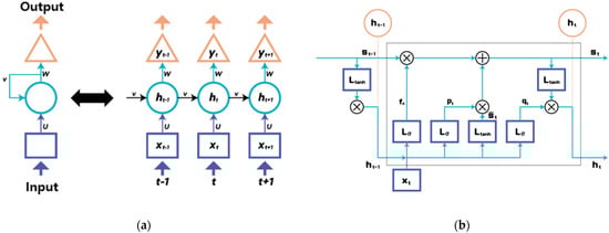
Figure 1. Architectures of the simple (a) RNN and (b) LSTM models.

The LSTM model consists of three structures, namely the forget, input, and out gates, and the formulas for each of these modules can be expressed as follows. LSTM models are widely used in various sequential data processing tasks owing to their ability to handle long-term dependencies and capture complex patterns over time [26,27]. Wang et al. presented a study using an LSTM model for power consumption prediction and anomaly detection. Kim et al. conducted a study to predict power consumption by connecting CNN-converged pattern extraction values to the LSTM network. This study was able to find out that feature extraction through CNN can be helpful for time series prediction.

$$f_t=\sigma (W_f·\left[h_{t-1}, x_t\right]+b_f)$$

(1)

$$i_t=\sigma \left(W_t·\left[h_{t-1}, x_t\right]+b_i\right), \widetilde{C_t}=\mathrm{t}\mathrm{a}\mathrm{n}\mathrm{h}(W_C·⌈h_{t-1}, x_t⌉+b_C)$$

(2)

$$C_t=f_t\ast C_{t-1}+i_t\ast {\tilde{C}}_t$$

(3)

$$o_t=\sigma \left(W_o\left[h_{t-1}, x_t\right]+b_o\right),h_t=o_t\ast \mathrm{t}\mathrm{a}\mathrm{n}\mathrm{h}\left(C_t\right)$$

(4)

2.1.3. GRU

The GRU is an RNN model designed to process sequential data, similar to the LSTM model [28]. Both the LSTM and GRU models show improvements over the traditional RNN for solving the gradient vanishing and exploding problems and capturing long-term dependencies in sequential data. The GRU is a simplified version of the LSTM model with fewer parameters and computations and has an update gate and a reset gate. Unlike the LSTM, which has a separate memory cell owing to a single memory gate, the GRU model does not explicitly use a separate cell for memory storage; instead, the hidden gate has the advantage of reducing the number of parameters by directly acting as a memory. Accordingly, the GRU has the advantage of faster learning because there are fewer parameters. Figure 2 shows the structure of the GRU. Mahjoub et al. studied application networks of GRU and LSTM for energy consumption predictions [29]. Li et al. presented a study linking the GRU network to an edge computing platform for short-term electricity demand forecasting [30]. In these papers, only ultra-short-term predictions or ultra-long-term aspects such as 1 day, 3 days, and 7 days were predicted.

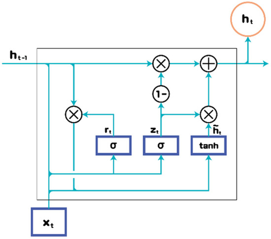
Figure 2. Typical architecture of the GRU.

2.1.4. TCN

One of the representative models of a CNN that can be used to predict time-series data is the TCN [31], which demonstrates longer effective memory and better performance than the LSTM. The existing convolutional layers are mainly used to extract low- or high-dimensional features from images and perform calculations based on them. The TCN is a structured model that is suitable for sequential data, identifying temporal patterns and dependencies of the input sequence using one-dimensional (1D) convolution, which is in the form of a 1D convolution layer. The TCN model uses 1D convolution to process the input sequence by sliding small filters to extract patterns, as well as using an extended convolution with gaps between the filters. The extended convolution effectively captures not only the short-term but also long-term data dependencies. In addition, the TCN has the advantage of being able to incorporate residual connections that solve the gradient vanishing problem and enable deep networks without performance degradations. Figure 3 shows the overall structure of the TCN, showing the graphical result of setting the convolution filter to 3 with dilation values of 1, 2, and 4 for each of the layers. The TCN can be implemented efficiently by having a wide receptive field based on the dilation value. Cai et al. studied a hybrid model linking the GRU and TCN models to predict short-term electricity demand [32].

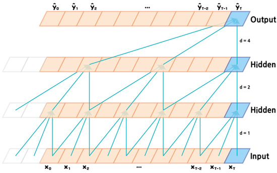
Figure 3. Architecture of the TCN.

2.1.5. Transformer

The transformer network is a model that has dramatically improved performance in the field of natural language processing (NLP) [33]. Figure 4a below shows the structure of the transformer. First, the encoder part in the transformer model is explained; input values applied to the encoder part first go through positional encoding. Existing RNN models or LSTM models involve sequential data inputs, but positional encoding plays an important role in a transformer network because the order information is not known if the order of the data is not input. Positional encoding converts the positional information and embedded data of the corresponding information in the sequence into a sine function and a cosine function before transferring them to the input of the next layer. This reflects the location information of the corresponding input data. For the input data, the encoder part consists of multihead attention, add and normalize, and feed-forward modules. Multihead attention is different from the attention method described above, wherein the attention score is calculated using the hidden states of the encoder and decoder; multihead attention obtains the attention score by calculating the vector input to the encoder and the entire vector input to the encoder. Figure 4b shows the scheme of the multihead attention. The decoder has a similar composition as the encoder but is different in that it contains a masked multihead attention module. In the case of the encoder, the entire input value can be seen, but in the case of a decoder, since the value to be input in the future is not known, it is masked so that it is not reflected. The more the layers of the encoder part of the transformer network model are stacked, the more the learnable parameters are stacked, which is advantageous for good performance. However, there is a downside in that the model is heavy. Saoud et al. conducted a study using wavelet transforms and transformers to predict occupant energy requirements [34]. However, this study focuses only on household power consumption prediction, and there is a lack of research on power consumption prediction in non-residential data.

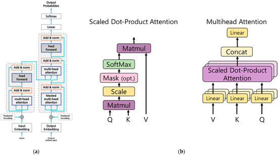
Figure 4. Architectures of the (a) transformer and (b) multihead attention modules.

3. Methodology

In this section, we define a time-series prediction problem for power consumption prediction. In addition, the dataset and performance indicators used for the experiments are summarized.

3.1. Dataset

Two datasets were used for the experiments in this study. The first dataset was actually collected from Chonnam National University (CNU) continuously at 1 h intervals for approximately 1 year and 3 months (1 January 2021 to 14 January 2022). The dataset contained power consumption data at 90 locations within CNU; there were 11,232 data for each location, and among these, the total power consumed at CNU building No. 7 was used for power consumption prediction. The second dataset was a high-voltage dataset continuously collected from factories at 1 h intervals for 2 years (1 August 2020 to 31 July 2022). Table 1 below shows the status of each dataset, which was subjected to min-max normalization for learning. The min-max regularization was performed as expressed in Equation (5). The dataset was constructed using the slide window method so that 168 data could be input during model learning.

$$x_{scaled}=\frac{x-x_{min}}{x_{max}-x_{min}}$$

(5)

Table 1. Dataset list.

Dataset	Environment	Length of Time Series	Attributions
CNU Dataset	University	11,232	Power Consumption
High-Voltage Dataset	Factory	17,001	Power Consumption

3.2. Performance Metrics

To assess the experimental performance in this work, the mean-squared error (MSE) and mean absolute error (MAE) performance indexes were used. The MSE is a common metric used to measure the mean-squared differences between the predicted and actual values in a dataset. Equation (6) represents the expression of the MSE performance index. The MAE is another commonly used metric to evaluate the performance of a predictive model and can be expressed as in Equation (7). Unlike the MSE, instead of squaring the differences between the predicted and actual values, the MAE uses the absolute value of the difference, which makes it more robust against outliers because it does not amplify the effects of the errors like the MSE. The choice of MSE and MAE as the performance indicators depends on the specific problem, nature of the data, and goals of the model. Therefore, it is important to select a model based on appropriate performance indicators according to the goal.

$$\mathrm{M}\mathrm{e}\mathrm{a}\mathrm{n} \mathrm{S}\mathrm{q}\mathrm{u}\mathrm{a}\mathrm{r}\mathrm{e} \mathrm{E}\mathrm{r}\mathrm{r}\mathrm{o}\mathrm{r}\left(\mathrm{M}\mathrm{S}\mathrm{E}\right)=\frac{1}{n}\sum _{i=1}^n{\left(\widehat{Y_i}-Y_i\right)}^2$$

(6)

$$\mathrm{M}\mathrm{e}\mathrm{a}\mathrm{n} \mathrm{A}\mathrm{b}\mathrm{s}\mathrm{o}\mathrm{l}\mathrm{u}\mathrm{t}\mathrm{e} \mathrm{E}\mathrm{r}\mathrm{r}\mathrm{o}\mathrm{r}\left(\mathrm{M}\mathrm{A}\mathrm{E}\right)=\frac{1}{n}\sum _{i=1}^n\left|\widehat{Y_i}-Y_i\right|$$

(7)

4. Experimental Results and Comparison

4.1. Deep Learning Model Setup

The deep learning models used in this study were the ANN, LSTM, GRU, TCN, and transformer models. The ANN model consists of two hidden layers, where the first layer has 32 nodes and second layer has 8 nodes. The LSTM model consists of two layers, where the first tier has 200 nodes and second tier has 150 nodes. The GRU model consists of two layers, and each layer has 103 nodes with the final layer consisting of linear unit activation functions. The TCN model is composed of one layer; the window size of the 1D convolution is 3, with the number of filters being 64 and kernel size being 3. The activation function of all models used the ReLU function. The transformer model has the advantage of good performance but has the disadvantage of being heavy owing to the large number of parameters. Table 2 is a table showing the network model configuration. In particular, the Transformer model used a transformer model composed of three layers and eight layers, as shown in Table 2, to compensate for the problem of transformers.

Table 2. Model construction of network.

Parameter	ANN	LSTM	GRU	Parameter	TCN	Parameter	Transformer-8 (TF-8)	Transformer-3 (TF-3)
Num_layer	2	2	2	Num_layer	1	Model dimension	256	32
Unit_layer1	32	200	103	1D_Conv_ window_Size	3
Return_seq	-	True	True	Filters	64	Num_head	8	4
Unit_layer2	8	150	103			Dropout(MultiHead Attention)	0.5	0
						Dropout(MLP)	0.5	0
						Number of Encoder	8	3

4.2. Training Methods

In this work, $\mathcal{i}$ was set to 168 and n was set from 0 to 23 to conduct the experiments. Based on time-series prediction, the problem can be expressed as Equation (8). The prediction problem was a problem of continuously predicting data from 1 h to 24 h. For example, in the problem of predicting 10 h, 168 time data were input, and the predicted value from 1 h to 10 h was later compared with the correct value. The implementation of the proposed method was achieved using the Keras library with TensorFlow backend. All models were trained and tested on four NVIDIA Quadro RTX A5000 24 GB GPUs.

$${\widehat{y}}_0,\dots ,{\widehat{y}}_n=f\left(x_0,\dots ,x_{167}\right), n=0, 1, 2,\dots , 23$$

(8)

4.3. Experimental Results and Analysis

The experiments proceeded with predictions according to values set from 1 to 24 h for the data entered for 168 h. The results with the best performances are indicated in bold red. The lower the MSE and MAE performance indexes, the better the results. Table 3 below shows the MSE performance of the CNU dataset. Table 4 below shows the MAE performance of the CNU dataset. Similarly, Table 5 and Table 6 below show the MSE and MAE performances of the high-voltage dataset.

Table 3. Deep learning model MSE performance of the CNU dataset.

Model	1 h	2 h	3 h	4 h	5 h	6 h	7 h	8 h	9 h	10 h	11 h	12 h
ANN	0.0023	0.0035	0.0049	0.005	0.0059	0.0067	0.007	0.0078	0.0201	0.0088	0.0086	0.0084
LSTM	0.002	0.0032	0.0043	0.0048	0.0067	0.007	0.0076	0.0083	0.0077	0.0095	0.0095	0.0109
GRU	0.0022	0.0038	0.0056	0.0072	0.0086	0.0077	0.0081	0.0092	0.0094	0.0101	0.0105	0.0109
TCN	0.002	0.0027	0.0036	0.0039	0.0059	0.0054	0.0067	0.0063	0.0081	0.0074	0.0071	0.0113
TF-8	0.0321	0.0337	0.0336	0.0333	0.0341	0.0326	0.0314	0.0317	0.0321	0.033	0.0331	0.0313
TF-3	0.0250	0.0246	0.0253	0.0298	0.0293	0.0297	0.0292	0.0302	0.0293	0.0294	0.0313	0.0311
Model	13 h	14 h	15 h	16 h	17 h	18 h	19 h	20 h	21 h	22 h	23 h	24 h
ANN	0.0096	0.0087	0.0091	0.0089	0.0094	0.0112	0.0092	0.0098	0.0093	0.0102	0.0103	0.0101
LSTM	0.0113	0.0114	0.0115	0.0115	0.0119	0.01	0.01	0.0107	0.0128	0.0133	0.0114	0.0097
GRU	0.0113	0.0113	0.0117	0.0117	0.0122	0.0118	0.0125	0.0124	0.0126	0.0127	0.0128	0.0128
TCN	0.0076	0.0079	0.0076	0.0115	0.0102	0.0107	0.0106	0.0127	0.0081	0.0111	0.009	0.0084
TF-8	0.0316	0.0313	0.0321	0.0314	0.1246	0.0324	0.0314	0.0322	0.0314	0.0318	0.0329	0.0341
TF-3	0.0316	0.0310	0.0316	0.0309	0.0316	0.0298	0.0316	0.0317	0.0298	0.0320	0.0316	0.0317

Table 4. Deep learning model MAE performance of the CNU dataset.

Model	1 h	2 h	3 h	4 h	5 h	6 h	7 h	8 h	9 h	10 h	11 h	12 h
ANN	0.0333	0.0417	0.0489	0.0481	0.0535	0.0567	0.0575	0.061	0.1019	0.0658	0.0646	0.0638
LSTM	0.0297	0.0369	0.042	0.0452	0.0533	0.0535	0.056	0.0585	0.0572	0.0647	0.0625	0.0687
GRU	0.0309	0.0395	0.0476	0.0542	0.0599	0.0589	0.0594	0.0651	0.0646	0.0669	0.0691	0.0702
TCN	0.0298	0.0343	0.0416	0.0423	0.0491	0.0509	0.0517	0.0537	0.062	0.0568	0.0568	0.0718
TF-8	0.1234	0.1257	0.1256	0.125	0.1264	0.1239	0.1231	0.1235	0.1234	0.1245	0.1247	0.1232
TF-3	0.1168	0.1155	0.1177	0.1290	0.1271	0.1285	0.1270	0.1303	0.1273	0.1279	0.1337	0.1329
Model	13 h	14 h	15 h	16 h	17 h	18 h	19 h	20 h	21 h	22 h	23 h	24 h
ANN	0.0691	0.0648	0.0668	0.066	0.0684	0.0753	0.0673	0.0701	0.0679	0.0716	0.072	0.0711
LSTM	0.0696	0.0701	0.071	0.0703	0.0709	0.0661	0.0681	0.0701	0.0757	0.0772	0.0715	0.067
GRU	0.0722	0.0711	0.073	0.0729	0.0747	0.0724	0.0764	0.0751	0.0762	0.0765	0.0768	0.0764
TCN	0.0593	0.061	0.0601	0.0734	0.0702	0.0718	0.0717	0.0765	0.062	0.0696	0.0664	0.0639
TF-8	0.1231	0.1232	0.1234	0.123	0.0331	0.1237	0.1231	0.1235	0.1233	0.1232	0.1243	0.1264
TF-3	0.1345	0.1327	0.1344	0.1324	0.1343	0.1291	0.1344	0.1346	0.1292	0.1355	0.1346	0.1349

Table 5. Deep learning model MSE performance of the high-voltage dataset.

Model	1 h	2 h	3 h	4 h	5 h	6 h	7 h	8 h	9 h	10 h	11 h	12 h
ANN	0.0011	0.0014	0.0015	0.0023	0.0020	0.0074	0.0025	0.0096	0.0074	0.0029	0.0029	0.0031
LSTM	0.0017	0.0037	0.0042	0.0048	0.0054	0.0053	0.0069	0.0063	0.0067	0.0065	0.0075	0.0075
GRU	0.0017	0.0034	0.0050	0.0048	0.0071	0.0051	0.0055	0.0058	0.0062	0.0073	0.0070	0.0071
TCN	0.0008	0.0011	0.0013	0.0015	0.0014	0.0015	0.0018	0.0020	0.0020	0.0020	0.0021	0.0020
TF-8	0.0818	0.0816	0.0827	0.0812	0.0817	0.0826	0.0814	0.081	0.0819	0.0819	0.0816	0.0824
TF-3	0.0294	0.0296	0.0295	0.0295	0.0296	0.0293	0.0293	0.0293	0.0295	0.0293	0.0295	0.0295
Model	13 h	14 h	15 h	16 h	17 h	18 h	19 h	20 h	21 h	22 h	23 h	24 h
ANN	0.0089	0.0029	0.0090	0.0027	0.0088	0.0035	0.0086	0.0034	0.0106	0.0038	0.0039	0.0042
LSTM	0.0074	0.0070	0.0069	0.0074	0.0077	0.0083	0.0071	0.0075	0.0081	0.0075	0.0077	0.0080
GRU	0.0070	0.0075	0.0075	0.0075	0.0079	0.0078	0.0079	0.0081	0.0080	0.0080	0.0082	0.0081
TCN	0.0022	0.0022	0.0020	0.0021	0.0024	0.0025	0.0025	0.0023	0.0022	0.0023	0.0025	0.0025
TF-8	0.0823	0.0819	0.0824	0.0824	0.0814	0.0817	0.0821	0.0826	0.0819	0.0808	0.0817	0.082
TF-3	0.0293	0.0294	0.0292	0.0295	0.0292	0.0293	0.0293	0.0294	0.0293	0.0293	0.0294	0.0293

Table 6. Deep learning model MAE performance of the high-voltage dataset.

Model	1 h	2 h	3 h	4 h	5 h	6 h	7 h	8 h	9 h	10 h	11 h	12 h
ANN	0.0494	0.079	0.0839	0.1211	0.0925	0.0841	0.0874	0.2001	0.1009	0.0897	0.0948	0.1745
LSTM	0.0258	0.0409	0.0442	0.0476	0.0499	0.0490	0.0570	0.0531	0.0542	0.0539	0.0587	0.0572
GRU	0.0229	0.0343	0.0449	0.0455	0.0580	0.0494	0.0500	0.0514	0.0525	0.0605	0.0566	0.0563
TCN	0.0149	0.0188	0.0203	0.0216	0.0216	0.0224	0.0248	0.0257	0.0257	0.0257	0.0270	0.0268
TF-8	0.1575	0.1575	0.1576	0.1576	0.1575	0.1575	0.1575	0.1576	0.1575	0.1575	0.1575	0.1575
TF-3	0.0969	0.0969	0.0969	0.0969	0.0969	0.0969	0.0970	0.0969	0.0969	0.0969	0.0969	0.0969
Model	13 h	14 h	15 h	16 h	17 h	18 h	19 h	20 h	21 h	22 h	23 h	24 h
ANN	0.0691	0.0648	0.0668	0.066	0.0684	0.0753	0.0673	0.0701	0.0679	0.0716	0.072	0.0711
LSTM	0.0696	0.0701	0.071	0.0703	0.0709	0.0661	0.0681	0.0701	0.0757	0.0772	0.0715	0.067
GRU	0.0722	0.0711	0.073	0.0729	0.0747	0.0724	0.0764	0.0751	0.0762	0.0765	0.0768	0.0764
TCN	0.0593	0.061	0.0601	0.0734	0.0702	0.0718	0.0717	0.0765	0.062	0.0696	0.0664	0.0639
TF-8	0.1231	0.1232	0.1234	0.123	0.0331	0.1237	0.1231	0.1235	0.1233	0.1232	0.1243	0.1264
TF-3	0.1345	0.1327	0.1344	0.1324	0.1343	0.1291	0.1344	0.1346	0.1292	0.1355	0.1346	0.1349

4.4. Summary of Experimental Results

Section 4.3 showed the experimental results of the deep learning models for the CNU and high-voltage datasets. In this section, the experimental results are summarized, and an optimal model for predicting power consumption based on time is presented. Table 7 below shows the experimental results of the CNU dataset; as shown, when the MSE performance indicators were summarized, the TCN model was the optimal model in 16 time zones. In the problem of predicting 1 h later, the LSTM was a joint optimal model. In addition, in the 5 h prediction problem, the ANN model was a co-optimal model; the LSTM model in three time zones and ANN model in seven time zones were the overall optimal models. When the MAE performance indicators were summarized, the TCN model was the optimal model in sixteen time zones, the ANN model was optimal in four time zones, the LSTM model was optimal in three time zones, and the TF-8 model was optimal in the 17 h prediction problem. In the MSE and MAE performances, the optimal models were different for prediction problems at 1 h, 5 h, 17 h, and 22 h; this suggests that there is a problem with outliers in the CNU dataset.

Table 7. Comparison of performances over time for the CNU dataset and derivation of the optimal model.

CNU Dataset, MSE
Time	1 h	2 h	3 h	4 h	5 h	6 h	7 h	8 h	9 h	10 h	11 h	12 h
Optimal Model	LSTM, TCN	TCN	TCN	TCN	TCN, ANN	TCN	TCN	TCN	LSTM	TCN	TCN	ANN
Time	13 h	14 h	15 h	16 h	17 h	18 h	19 h	20 h	21 h	22 h	23 h	24 h
Optimal Model	TCN	TCN	TCN	ANN	ANN	LSTM	ANN	ANN	TCN	ANN	TCN	TCN
CNU Dataset, MAE
Time	1 h	2 h	3 h	4 h	5 h	6 h	7 h	8 h	9 h	10 h	11 h	12 h
Optimal Model	LSTM	TCN	TCN	TCN	TCN	TCN	TCN	TCN	LSTM	TCN	TCN	ANN
Time	13 h	14 h	15 h	16 h	17 h	18 h	19 h	20 h	21 h	22 h	23 h	24 h
Optimal Model	TCN	TCN	TCN	ANN	TF-8	LSTM	ANN	ANN	TCN	TCN	TCN	TCN

Table 8 below shows the experimental results of the high-voltage dataset; when the MSE and MAE performance indicators were summarized, the TCN model was overwhelmingly the optimal model in terms of numbers over the entire time period. It was found that the TCN model based on the convolutional layer was able to better solve the data characteristics and problem complexity within the high-voltage dataset.

Table 8. Comparison of performances over time for the high-voltage dataset and derivation of the optimal model.

High-Voltage Dataset, MSE
Time	1 h	2 h	3 h	4 h	5 h	6 h	7 h	8 h	9 h	10 h	11 h	12 h
Optimal Model	TCN	TCN	TCN	TCN	TCN	TCN	TCN	TCN	TCN	TCN	TCN	TCN
Time	13 h	14 h	15 h	16 h	17 h	18 h	19 h	20 h	21 h	22 h	23 h	24 h
Optimal Model	TCN	TCN	TCN	TCN	TCN	TCN	TCN	TCN	TCN	TCN	TCN	TCN
High-Voltage Dataset, MAE
Time	1 h	2 h	3 h	4 h	5 h	6 h	7 h	8 h	9 h	10 h	11 h	12 h
Optimal Model	TCN	TCN	TCN	TCN	TCN	TCN	TCN	TCN	TCN	TCN	TCN	TCN
Time	13 h	14 h	15 h	16 h	17 h	18 h	19 h	20 h	21 h	22 h	23 h	24 h
Optimal Model	TCN	TCN	TCN	TCN	TCN	TCN	TCN	TCN	TCN	TCN	TCN	TCN

In this section, the results of the experiments are summarized, and the optimal model for predicting power consumption is presented for each dataset. Based on the dataset, the model with the best performance over the entire time period and the best model on aver-age were compared. The optimal model is indicated in bold text. Table 9 below is organized based on the experimental results of the CNU dataset. In the results of the MSE experiment, it is seen that the LSTM and TCN models were the best when the best performance was required, and the TCN model was the best on average. In the results of the MSE experiment, the LSTM and TCN models, which both show maximum performances, produced 10–15% better performances than the ANN and GRU models, and it is seen that the average performance was good from at least 10% for a maximum of four times. In the results of the MAE experiment, it is seen that the LSTM model produced the best performance and that the TCN model was good on average. The LSTM model, which shows the maximum performance in the MAE experiment results, has similar performance to the TCN model, but shows improved performance by 4–12% compared to the ANN and GRU models and by 11–388% compared to the transformer model. On average, the TCN model outperformed the other models by up to 4–221%.

Table 9. CNU dataset performance comparisons by model and optimal model arrangement.

Model	CNU Dataset, MSE				CNU Dataset, MAE
	Min.	Percentage	Avg.	Percentage	Min.	Percentage	Avg.	Percentage
ANN	0.0023	1.15	0.00853	1.102	0.0333	1.121	0.06363	1.085
LSTM	0.002	1	0.00904	1.167	0.0297	1	0.06149	1.049
GRU	0.0022	1.1	0.00996	1.286	0.0309	1.04	0.06583	1.123
TCN	0.002	1	0.00774	1	0.0298	1.003	0.05861	1
TF-8	0.0313	15.65	0.03622	4.678	0.0331	1.114	0.12024	2.051
TF-3	0.0246	12.3	0.02996	3.87	0.1155	3.888	0.12979	2.214

Table 10 below is organized based on the MSE results of the high-voltage dataset. For both the MSE and MAE experimental results, the TCN model is the optimal model. In the results of the MSE experiment, the TCN model with the highest performance showed twice the performance of the ANN, LSTM, or GRU models. On average, it was seen that the performance was about 2–3 times better. In the MAE experiment results, the TCN model shows good performance from a minimum of 49% to a maximum of 650%. On average, it is seen that the performance was good, ranging from a minimum of 21% to a maximum of 303%.

Table 10. High-voltage dataset performance comparisons by model and optimal model arrangement.

Model	High-Voltage Dataset, MSE				High-Voltage Dataset, MAE
	Min.	Percentage	Avg.	Percentage	Min.	Percentage	Avg.	Percentage
ANN	0.0011	1.442	0.0048	2.386	0.02229	1.495	0.05478	1.215
LSTM	0.0017	2.111	0.0066	3.263	0.02589	1.737	0.05999	1.331
GRU	0.0017	2.07	0.0067	3.315	0.02294	1.538	0.06152	1.365
TCN	0.0008	1	0.0020	1	0.01491	1	0.04507	1
TF-8	0.0808	97.939	0.0818	40.51	0.0331	2.22	0.13682	3.035
TF-3	0.0292	35.47	0.0294	14.565	0.09693	6.502	0.1152	2.555

Based on these experimental results, the characteristics of the dataset were analyzed. The CNU dataset has a special characteristic of being from a school; conversely, the high-voltage dataset has the specificity of being from a factory. Figure 5 below is a visualization of each dataset. From Figure 5a, the CNU dataset has periodic characteristics, whereas the high-voltage dataset (Figure 5b) has periodic peaks owing to situations such as facility operation in the factory. The X-axis of Figure 5 represents power consumption, and the horizontal axis represents the order of time. A total of 2000 data were visualized in a random part within the dataset.

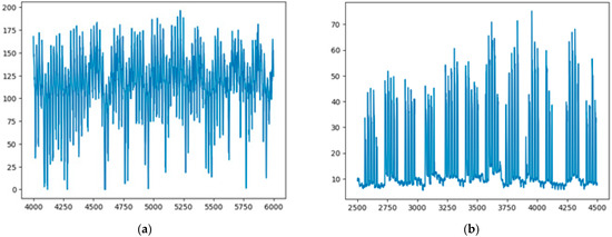
Figure 5. Visualization of the (a) CNU and (b) high-voltage datasets.

5. Conclusions

In this study, we experimented with the ANN, LSTM, and GRU as well as TCN and transformer models for two sets of data, namely the CNU and high-voltage datasets. The transformer model had the disadvantage of being heavy, so a lightweight three-layer model was applied. In addition, detailed power predictions were carried out in 1 h increments from 1 to 24 h. Thus, it was possible to derive an optimal model for each time period and an optimal model for the maximum and average performances. For the dataset showing periodic patterns, the LSTM model was the best at predicting information 1 h later, and for the dataset containing peak states, the TCN model was the best. It was found that the TCN model was the best on average, from 1 to 24 h. The datasets used in this study involve special environments, such as schools and factories, rather than general households. Non-residential datasets are an important area for energy management and energy efficiency improvement. In this paper, we can suggest the direction of the optimal model in the non-residential environment dataset. The problem that can derive the maximum performance in this paper is the prediction problem after 1 h. In the future, through hourly hyper parameter optimization, it will be possible to derive a more accurate performance not only after 1 h, but also from 2 h to 24 hours’ prediction problems compared to prediction problems after 1 h. In the future, we will research technologies that can improve energy management efficiency through research using non-residential data household electricity datasets and research using datasets including external factors that affect power consumption, such as temperature and humidity.

References

- Tvaronavičienė, M.; Baublys, J.; Raudeliūnienė, J.; Jatautaitė, D. Chapter 1—Global energy consumption peculiarities and energy sources: Role of renewables. In Energy Transformation towards Sustainability; Tvaronavičienė, M., Ślusarczyk, B., Eds.; Elsevier: Amsterdam, The Netherlands, 2020; pp. 1–49. ISBN 9780128176887. [Google Scholar]
- Kober, T.; Schiffer, H.-W.; Densing, M.; Panos, E. Global energy perspectives to 2060—WEC’s World Energy Scenarios 2019. Energy Strat. Rev. 2020, 31, 100523. [Google Scholar] [CrossRef]
- Bilgen, S. Structure and environmental impact of global energy consumption. Renew. Sustain. Energy Rev. 2014, 38, 890–902. [Google Scholar] [CrossRef]
- IIris, Ç.; Lam, J.S.L. A review of energy efficiency in ports: Operational strategies, technologies and energy management systems. Renew. Sustain. Energy Rev. 2019, 112, 170–182. [Google Scholar] [CrossRef]
- Desislavov, R.; Martínez-Plumed, F.; Hernández-Orallo, J. Compute and energy consumption trends in deep learning inference. arXiv 2021, arXiv:2109.05472. [Google Scholar]
- Zhou, K.; Yang, S. Understanding household energy consumption behavior: The contribution of energy big data analytics. Renew. Sustain. Energy Rev. 2016, 56, 810–819. [Google Scholar] [CrossRef]
- Somu, N.; MR, G.R.; Ramamritham, K. A deep learning framework for building energy consumption forecast. Renew. Sustain. Energy Rev. 2021, 137, 110591. [Google Scholar] [CrossRef]
- Khalil, M.; McGough, A.S.; Pourmirza, Z.; Pazhoohesh, M.; Walker, S. Machine Learning, Deep Learning and Statistical Analysis for forecasting building energy consumption—A systematic review. Eng. Appl. Artif. Intell. 2022, 115, 105287. [Google Scholar] [CrossRef]
- Chou, J.-S.; Tran, D.-S. Forecasting energy consumption time series using machine learning techniques based on usage patterns of residential householders. Energy 2018, 165, 709–726. [Google Scholar] [CrossRef]
- Liang, F.; Yu, A.; Hatcher, W.G.; Yu, W.; Lu, C. Deep learning-based power usage forecast modeling and evaluation. Procedia Comput. Sci. 2019, 154, 102–108. [Google Scholar] [CrossRef]
- García-Martín, E.; Rodrigues, C.F.; Riley, G.; Grahn, H. Estimation of energy consumption in machine learning. J. Parallel Distrib. Comput. 2019, 134, 75–88. [Google Scholar] [CrossRef]
- Jiang, W. Deep learning based short-term load forecasting incorporating calendar and weather information. Internet Technol. Lett. 2022, 5, e383. [Google Scholar] [CrossRef]
- Xu, A.; Tian, M.-W.; Firouzi, B.; Alattas, K.A.; Mohammadzadeh, A.; Ghaderpour, E. A New Deep Learning Restricted Boltzmann Machine for Energy Consumption Forecasting. Sustainability 2022, 14, 10081. [Google Scholar] [CrossRef]
- Hong, Y.; Wang, D.; Su, J.; Ren, M.; Xu, W.; Wei, Y.; Yang, Z. Short-Term Power Load Forecasting in Three Stages Based on CEEMDAN-TGA Model. Sustainability 2023, 15, 11123. [Google Scholar] [CrossRef]
- Chen, Z.; Wang, C.; Lv, L.; Fan, L.; Wen, S.; Xiang, Z. Research on Peak Load Prediction of Distribution Network Lines Based on Prophet-LSTM Model. Sustainability 2023, 15, 11667. [Google Scholar] [CrossRef]
- Makala, B.; Bakovic, T. Artificial Intelligence in the Power Sector; International Finance Corporation: Washington, DC, USA, 2020. [Google Scholar]
- Wu, Q.; Ren, H.; Shi, S.; Fang, C.; Wan, S.; Li, Q. Analysis and prediction of industrial energy consumption behavior based on big data and artificial intelligence. Energy Rep. 2023, 9, 395–402. [Google Scholar] [CrossRef]
- Alzoubi, A. Machine learning for intelligent energy consumption in smart homes. Int. J. Comput. Inf. Manuf. (IJCIM) 2022, 2, 62–75. [Google Scholar] [CrossRef]
- Kim, T.; Cho, S. Predicting residential energy consumption using CNN-LSTM neural networks. Energy 2019, 182, 72–81. [Google Scholar] [CrossRef]
- Khan, N.; Haq, I.U.; Khan, S.U.; Rho, S.; Lee, M.Y.; Baik, S.W. DB-Net: A novel dilated CNN based multi-step forecasting model for power consumption in integrated local energy systems. Int. J. Electr. Power Energy Syst. 2021, 133, 107023. [Google Scholar] [CrossRef]
- Ryu, S.; Noh, J.; Kim, H. Deep Neural Network Based Demand Side Short Term Load Forecasting. Energies 2017, 10, 3. [Google Scholar] [CrossRef]
- Amarasinghe, K.; Marino, D.L.; Manic, M. Deep neural networks for energy load forecasting. In Proceedings of the 2017 IEEE 26th International Symposium on Industrial Electronics (ISIE), Edinburgh, UK, 19–21 June 2017; pp. 1483–1488. [Google Scholar]
- Yazdan, M.M.S.; Khosravia, M.; Saki, S.; Mehedi, M.A.A. Forecasting Energy Consumption Time Series Using Recurrent Neural Network in Tensorflow. Preprints 2022, 2022090404. [Google Scholar]
- Sachin, M.M.; Baby, M.P.; Ponraj, A.S. Analysis of Energy Consumption Using RNN-LSTM and ARIMA Model. J. Phys. Conf. Ser. 2020, 1716, 012048. [Google Scholar] [CrossRef]
- Hochreiter, S.; Schmidhuber, J. Long Short-Term Memory. Neural Comput. 1997, 9, 1735–1780. [Google Scholar] [CrossRef] [PubMed]
- Wang, X.; Zhao, T.; Liu, H.; He, R. Power consumption predicting and anomaly detection based on long short-term memory neural network. In Proceedings of the 2019 IEEE 4th International Conference on Cloud Computing and Big Data Analysis (ICCCBDA), Chengdu, China, 12–15 April 2019; pp. 487–491. [Google Scholar]
- Torres, J.F.; Martínez-Álvarez, F.; Troncoso, A. A deep LSTM network for the Spanish electricity consumption forecasting. Neural Comput. Appl. 2022, 5, 10533–10545. [Google Scholar] [CrossRef] [PubMed]
- Chung, J.; Gulcehre, C.; Cho, K.; Bengio, Y. Empirical evaluation of gated recurrent neural networks on sequence modeling. arXiv 2014, arXiv:1412.3555. [Google Scholar]
- Mahjoub, S.; Chrifi-Alaoui, L.; Marhic, B.; Delahoche, L. Predicting Energy Consumption Using LSTM, Multi-Layer GRU and Drop-GRU Neural Networks. Sensors 2022, 22, 4062. [Google Scholar] [CrossRef] [PubMed]
- Li, X.; Zhuang, W.; Zhang, H. Short-Term Power Load Forecasting Based on Gate Recurrent Unit Network and Cloud Computing Platform. In Proceedings of the 4th International Conference on Computer Science and Application Engineering, Sanya, China, 20 October 2020; pp. 1–6. [Google Scholar]
- Bai, S.; Kolter, J.Z.; Koltun, V. An empirical evaluation of generic convolutional and recurrent networks for sequence modeling. arXiv 2018, arXiv:1803.01271. [Google Scholar]
- Cai, C.; Li, Y.; Su, Z.; Zhu, T.; He, Y. Short-Term Electrical Load Forecasting Based on VMD and GRU-TCN Hybrid Network. Appl. Sci. 2022, 12, 6647. [Google Scholar] [CrossRef]
- Vaswani, A.; Shazeer, N.; Parmar, N.; Uszkoreit, J.; Jones, L.; Gomez, A.N.; Kaiser, L.; Polosukhin, I. Attention is All You Need. In Proceedings of the 31st International Conference on Neural Information Processing Systems, NIPS’17, Long Beach, CA, USA, 4–9 December 2017; Curran Associates Inc.: Red Hook, NY, USA, 2017; pp. 6000–6010. [Google Scholar]
- Saoud, L.S.; Al-Marzouqi, H.; Hussein, R. Household Energy Consumption Prediction Using the Stationary Wavelet Transform and Transformers. IEEE Access 2022, 10, 5171–5183. [Google Scholar] [CrossRef]
Disclaimer/Publisher’s Note: The statements, opinions and data contained in all publications are solely those of the individual author(s) and contributor(s) and not of MDPI and/or the editor(s). MDPI and/or the editor(s) disclaim responsibility for any injury to people or property resulting from any ideas, methods, instructions or products referred to in the content. |
© 2023 by the authors. Licensee MDPI, Basel, Switzerland. This article is an open access article distributed under the terms and conditions of the Creative Commons Attribution (CC BY) license (https://creativecommons.org/licenses/by/4.0/).