Intelligent Risk Prediction System in IoT-Based Supply Chain Management in Logistics Sector

Abstract

The Internet of Things (IoT) has resulted in substantial advances in the logistics sector, particularly in logistics storage management, communication systems, service quality, and supply chain management. The goal of this study is to create an intelligent supply chain (SC) management system that provides decision support to SC managers in order to achieve effective Internet of Things (IOT)-based logistics. Current research on predicting risks in shipping operations in the logistics sector during natural disasters has produced a variety of unexpected findings utilizing machine learning (ML) algorithms and traditional feature-encoding approaches. This has prompted a variety of concerns regarding the research’s validity. These previous attempts, like many others before them, used deep neural models to gain features without requiring the user to maintain track of all of the sequence information. This paper offers a hybrid deep learning (DL) approach, convolutional neural network (CNN) + bidirectional gating recurrent unit (BiGRU), to lessen the impact of natural disasters on shipping operations by addressing the question, “Can goods be shipped from a source location to a destination?”. The suggested DL methodology is divided into four stages: data collection, de-noising or pre-processing, feature extraction, and prediction. When compared to the baseline work, the proposed CNN + BiGRU achieved an accuracy of up to 94%.

1. Introduction

The term “supply chain” (SC) refers to the network of interconnected human, mechanical, activity, resource, and technical nodes involved in the creation and distribution of a product. It includes everything from the initial supply of raw materials or partially completed goods to the producer to the final delivery of the service or commodities to the final consumer or client [1]. To ensure a continued supply of goods and resources, competent management of supply chain activities is required [1]. In this regard, decision-makers must organize a number of tasks related to the acquisition and transportation of material resources, product delivery, and the delivery of goods and materials at the proper location and at a suitable time. Natural disasters such as earthquakes and floods, as well as the COVID-19 pandemic, have significantly affected the usual flow of products and commodities, including necessities such as personal protective equipment (PPE), medical facial masks, ventilation supplies, and ventilatory assistance [2]. Such circumstances may impair the smooth passage of commodities between divisions. As a result, it is obvious that acquiring this expertise will aid in dealing with these challenges.

1.1. Research Motivation

If an enterprise wants to continue running efficiently and successfully, SC risks [3] and disruptions must be handled as soon as possible. Early detection of risks is undeniably advantageous, both in terms of being better prepared to deal with catastrophic events and of limiting the impact of interruptions on the SC as a whole. The faster decision-makers can recognize or predict a potential threat to the SC, the more effectively they will be able to limit the risk’s negative effects by implementing an adequate prevention strategy [4]. At the beginning of the risk detection and evaluation plan, it is critical to identify both external risks (such as the risk of demand versus supply, environmental risks, and corporate risks) and internal hazards (such as the risk of production, the risk of organizing and monitoring, and the risk of prevention and backup [5].

The work by [1] used ML classification techniques to predict possible risks in the distribution of vaccines. Unlike the cutting-edge ML model [1], which learned sequential association [4], it used ML classification methods to extract features in a more traditional manner. The worldwide data links cannot be considered. As a result, the ML model fails to effectively reduce the risks connected with the vaccine SC.

DL combines a complete collection of feature-embedding techniques to proactively train from data and reliably anticipate future events [6,7]. It has been used in a variety of applications over the years, including stock market predictions [6], evaluating academic accomplishments [7], developing predictive models [3], and classifying literature [8], among others [5]. As a result, data scientists work hard to develop real-world solutions that can assist network administrators in more accurately forecasting SC hazards in the logistics sector [3]. As a result, it is critical to explore and deploy cutting-edge composite DL models based on benchmark data for precise risk prediction in SC.

1.2. Problem Statement

To address the aforementioned constraints, we implemented the CNN + BiGRU architecture, which combines a convolutional neural network and a bidirectional gated recurrent unit. The CNN model has been shown to be effective at accurately categorising SC risks. Furthermore, the BiGRU model makes use of context-sensitive data by employing both forward and backward GRU.

This study focuses on the problem of predicting SC risk using DL methodologies. The goal of this research is to build a classifier that can assign a binary label Si ∈ {0, 1} to all SC data Di in a given input set D = {D1, D2, D3, …, Dn}. Label 1 indicates that the relevant shipping is possible, but label 0 indicates that the products cannot be transported.

In this study, we run experiments on a wide range of traditional ML methods as well as cutting-edge DL techniques such as long short-term memory (LSTM), bidirectional LSTM (BiLSTM), CNNs, and a recurrent neural network (RNN). Traditional ML classification algorithms rely on bag-of-words-inspired methods such as term frequency–inverse document frequency (TF-IDF) and count vectorizer, but deep neural network models adhere to the concept of a content-embedding-based feature representation scheme.

A primary goal of the proposed system is to effectively extract features using a convolutional neural network (CNN) model. By incorporating contextual data in both the forward and reverse dimensions, the BiGRU model efficiently predicts SC hazards.

1.3. Research Questions

To accurately forecast supply chain risks in the logistics industry, we focus on the following research questions (see Table 1).

Table 1. Research questions.

Research Questions	Motivation
RQ1: When given a benchmark data set, how accurately does the CNN + BiGRU composite DL model predict supply chain risks in the logistics sector?	Deep neural network models, specifically CNN + BiGRU, are being investigated and put into use in order to forecast supply chain risks in the logistics sector.
RQ2: How can we contrast the proposed CNN + BiGRU model with classical ML methods?	To examine the efficacy of traditional feature representation methods, such as Bag of Words (BOW), using ML classifiers.
RQ3: How can we evaluate the efficacy of the proposed method in predicting supply chain risks in the logistics sector in relation to benchmark research and other DL methods?	To evaluate and contrast the outcomes of the proposed CNN + BiGRU DL model with those of competing approaches, evaluation metrics such as precision, recall, F1-score, and accuracy will be used.

1.4. Research Contributions

This paper makes three significant contributions:

(i)

In particular, we present a multi-model hybrid DL technique based on CNN and BIGRU for forecasting delivery timing and status. (For example SC hazards.)

(ii)

Choosing one of several more complex DL techniques that shows the most potential in terms of performance while being taught.

(iii)

Displaying the models’ performance on advanced DL networks.

The following is the sequence in which the remaining elements of the research are presented: Section 2 goes over some previously published works on intelligent supply chain prediction. Section 3 depicts the suggested DL methods for shipment export forecasting, as well as each stage of the procedure. Section 4 presents the results of the experiments as well as the commentary on the observed results, and Section 5 presents the conclusions.

2. Related Work

2.1. Machine Learning Techniques for Intelligent Supply Chain Risk Prediction Systems

Artificial neural networks, Bayesian learning, big data, and support vector machines (SVM) are common ML methods in the field [9]. ANN was used to investigate the factors that influence how harmful SC is. A model was created using back propagation, a neural network training approach (BPNN). BPNN is useful because it can handle problems that are exceedingly non-linear or intricate. A risk assessment indicator approach was established with the help of this model, providing organizations with a solid decision-making tool when it comes to SC risk management. They argued, for example, that their proposed approach can serve as an example for growing finance businesses. Liu and Huang [10] have proposed an ensemble SVM to assess vulnerability in the SC financial system. The model was used to analyse the financial data of China’s publicly traded companies (SCs). The firm figures contained numerous outliers. A noise reduction approach based on fuzzy grouping and principal component analysis was used to remove unwanted sounds and provide the cleanest datasets possible.

2.2. Deep Learning Techniques for Intelligent Supply Chain Risk Prediction Systems

Bassiouni et al. [3] proposed a DL solution to lessen the risk of a shipment going missing by determining in advance “if a shipment can be exported from one source to another”, despite the COVID-19 pandemic’s restrictions. The proposed DL techniques are divided into four key phases: data gathering, noise reduction or preparatory processing, feature extraction, and categorization. Based on the computational results, one of the proposed temporal convolutional network (TCN) models is virtually perfect at estimating the risk of transportation to a certain place within the constraints imposed by COVID-19. However, in this article, the number of dispatches used for training, testing, and validation was limited. It is possible to try to extend or increase the total number of shipments. Xu et al. [11] investigated the development of a deep learning method for forecasting variable demand for dockless bicycle rentals. A DL technique has been developed utilizing an LSTM artificial neural network (LSTM-NN) to forecast bike-sharing service and attractiveness journey outputs over varied time periods. The data were gathered in a central area of Nanjing. The success of the LSTM-NN was evaluated using a variety of mathematical models and ML approaches. In terms of prediction precision, the results showed that the LSTM-NN outperformed the conventional approaches. A DL model based on the LSTM design was proposed by [12] to anticipate the expansion rates of distribution networks during the global COVID-19 outbreak. It was predicted that there would be excessive demand for services and goods based on data from Google’s trend service and administrative decisions regarding the shutdown. Multiple methodologies were employed for forecasts based on machine learning and deep learning. Their findings showed that the DL strategy based on the LSTM had the highest forecasting accuracy when compared to classical ML and time-series prediction methods. Using MATLAB, a SC risk evaluation model based on a BP neural network was created and assessed [13]. The outcomes of the simulation show that the suggested BP neural network model performs remarkably well in SC risk evaluation, with a maximum relative error of 0.03076923%. The estimated maximum relative error is substantially greater when employing the method of analytical hierarchy (AHP), coming in at 57.41%. In comparison to the AHP model, the BP-neural-network-based SC risk evaluation model exhibits a higher level of matching efficiency.

2.3. Miscellaneous Techniques for Intelligent Supply Chain Risk Prediction Systems

In a research study carried out by [1] they developed an astute VSC management system that offers decision-making assistance for the management of the vaccine SC in the context of the COVID-19 pandemic. The integration of blockchain, the internet of things (IoT), and machine learning within the system provides a comprehensive solution to the three challenges encountered in the VSC. The utilization of blockchain technology’s transparency feature fosters trust and confidence among involved parties. The utilization of the Internet of Things (IoT) for the purpose of continuous tracking of vaccine status is instrumental in ensuring the quality of vaccines. The utilization of ML techniques enables the prediction of vaccine demand and the conduct of sentiment assessments on vaccine feedback, thereby facilitating the enhancement of vaccines by enterprises. The results are promising; but, by combining this with more advanced approaches such as transfer learning, additional improvement is possible. A questionnaire has been developed specifically for measuring the risks in the context of intelligent production, and a conceptual framework has been created to identify risks associated with the digital SC [14]. Using multilevel clustering analysis, an improved risk evaluation model was built, which incorporates 22 risk indicators drawn from a collection of 814 valid specimens. For the smart manufacturing supply network, the weighted information entropy technique was also employed to determine the weights of the aforementioned dangers. Simulation was used to validate the correctness of these risk variables and weights, demonstrating their usefulness. Palmer et al. [15] present a reference ontology that operates as a framework for risk evaluation in product-service networks in the context of global production chains. Their work aims to speed up the development of information systems by creating a common foundation that enhances interoperability and makes it easier for information to flow freely between disparate systems and organizations. The proposed reference ontology aims to accelerate the development of information systems by providing a consistent framework for risk assessment in this domain. The work performed by [16] aims to improve the order picking process without requiring more investments in software, workers, tools, or inventory. To overcome this, data from the Warehouse Management System (WMS) is extracted and prepared. Big data analysis and product grouping are carried out utilizing Tableau software and the obtained data. The purpose of this analysis is to solve the product allocation problem (PAP). The success of the proposed modifications can be evaluated by calculating and comparing the picking time between the present reference case and the newly analysed one. Table 2 presents a review of selected studies.

Table 2. Comparison of studies for intelligent supply chain risk prediction systems.

Study	Objectives	Techniques/Methods	Results	Limitations
Liu and Huang [10]	-	Machine learning (ensemble SVM)	Acc: 83.26%	This study simply applied ensemble SVM, whereas the investigation could apply some additional methods to increase accuracy.
Cai et al. [9]	-	Machine learning (SVM)	The linear approach outperforms the other models with regard to precision, recall, and accuracy.	Models are implemented with a limited dataset.
Xu et al. [11]	-	Deep learning (LSTM-NN)	The model produces satisfactory outcomes.	There is still room for enhancements to the framework by incorporating feature selection with DL models
Lorenc et al. [16]	-	Deep learning (LSTM)	LSTM improves precision, reduces runtimes, and optimizes memory utilization.	The proposed model lacks handling contextual information
Bassiouni et al. [3]	-	Deep learning (TCN)	Based on computational results, the suggested model (i.e., TCN) is ideal at calculating the risk of transportation to a certain location within the COVID-19 limitations.	There are a limited number of dispatches available for training, testing, and validation. It is necessary to raise or extend the overall quantity of shipments.
Pan et al. [13]	Supply chain risk evaluation	Deep learning (BP) neural network	Maximum relative error (0.03076923%)	The integration of feature selection and hybrid DL approaches can increase model performance.
Hu et al. [1]	Vaccine supply chain (SC) in the context of the COVID-19 pandemic	Blockchain, Internet of Things (IoT) Machine learning	The results are promising (Acc: 87.23%, Pre: 85.51%, Rec: 86.85%, F1-score: 87.34%)	By combining it with more advanced approaches such as transfer learning, additional improvement is possible.
Liu, et al. [14]	To identify risks associated with the digital supply chain	Multilevel clustering analysis Improved risk evaluation model	The model produced positive results and had high predictive power.	Lack of automated and enhanced risk assessment methods based on hybrid deep learning.
Palmer et al. [15]	Supply chain risk evaluation	Reference ontology method	The proposed models have an accuracy range of 80–86% and an average recall of 75–83%.	A combination of different ML and DL methods is required for efficient risk prediction in supply chains.

Research Gap:

According to our review of the available literature, SC risk modelling employs a variety of cutting-edge methods and tools, including ML and DL approaches. Various statistical, machine learning, graphical representation, and data mining methods have been investigated for the purpose of predicting SC risk. Furthermore, it has been reported that SC risk prediction using deep learning is an emerging research topic that enables effective processing and analysis of SC hazards in the logistics business. The majority of these methods, however, are based on traditional DL methodologies. Investigating and applying composite DL approaches for SC risk prediction is thus critical, and this is what this work attempts to do.

3. Proposed Methodology

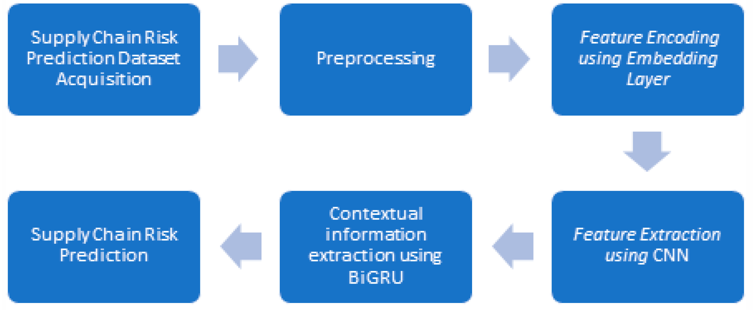
The suggested method can be broken down into several important modules (see Figure 1), which are as follows: (i) Supply chain risk prediction dataset acquisition; (ii) preprocessing; (iii) feature encoding using an embedding layer; (iv) feature extraction using a CNN Layer; and (v) model development. The following is a description of each module’s specifics in more detail.

Figure 1. Overview of the proposed system.

3.1. Supply Chain Risk Prediction Dataset Acquisition

Kaggle [17], a popular online library popular among the machine learning and data science communities, provided the raw data for this study. There are a plethora of publicly available data sets accessible from this repository. The selected data collection is titled “US Supply Chain Information for COVID-19” [17]. Transferable shipments from an origin to a recipient are included in this dataset. In the spreadsheet regarding the North American business classification scheme, the 547,661 packages in this dataset are divided into a variety of industries, including mining (apart from petroleum and natural gas), food production, textile factories, paper, wooden manufacturing of items, and a number of others [17]. Every shipment has twenty different features that describe various aspects of the dispatch (see Table 3).

Table 3. Description of dataset attributes [17].

Field	Description	Valid Values	Type	Length
SHIPMT_ID	Shipment identifier	0000001–4,547,661	CHAR	7
ORIG_STATE	FIPS state code of shipment origin	01–56	CHAR	2
ORIG_MA	Metro area of shipment origin	See .csv file	CHAR	5
ORIG_CFS_AREA	CFS area of shipment origin	Concatenation of ORIG_STATE and ORIG_MA	CHAR	8
DEST_STATE	FIPS state code of shipment destination	01–56	CHAR	2
DEST_MA	Metro area of shipment destination	See .csv file	CHAR	5
DEST_CFS_AREA	CFS area of shipment destination	Concatenation of DEST_STATE and DEST_MA	CHAR	8
NAICS	Industry classification of shipper	See .csv file	CHAR	6
QUARTER	Quarter of 2012 in which the shipment occurred	1, 2, 3, 4	CHAR	1
SCTG	2-digit SCTG commodity code of the shipment	See .csv file	CHAR	5
MODE	Mode of transportation of the shipment	See .csv file	CHAR	2
SHIPMT_VALUE	Value of the shipment in dollars	$0–999,999,999	NUM	8
SHIPMT_WGHT	Weight of the shipment in pounds	0–999,999,999	NUM	8
SHIPMT_DIST_GC	Great circle distance between shipment origin and destination (in miles)	0–99,999	NUM	8
SHIPMT_DIST_ROUTED	Routed distance between shipment origin and destination (in miles)	0–99,999	NUM	8
TEMP_CNTL_YN	Temperature controlled shipment—Yes or No	Y, N	CHAR	1
EXPORT_YN	Export shipment—Yes or No	Y, N	CHAR	1
EXPORT_CNTRY	Export final destination	C = Canada	CHAR	1
-	-	M = Mexico	-	-
-	-	O = Other	-	-
HAZMAT	Hazardous material (HAZMAT) code	P = class 3 HAZMAT (flammable liquids)	CHAR	1
-	-	H = other HAZMAT	-	-
-	-	N = not HAZMAT	-	-
WGT_FACTOR	Shipment tabulation weighting factor	0–999,999	NUM	8

3.2. Pre-Processing

The pre-processing process is reliant on a number of primary steps.

Eliminating incomplete entries: We started by removing any records that were incomplete, meaning deliveries that lacked important dates or statuses or that had incorrect information. The accessibility of alphanumeric identification for both suppliers and parts influenced this decision. The initial stage involved eliminating the columns that pertained to identical attributes and the columns containing distinctive identifiers. The columns that met the aforementioned requirements were eliminated. The columns that were removed from the dataset were “shipment id”, “concatenation of the original state and metro area”, and “concatenation of the destination state and metro area”. The initial outcome of the procedure was a total of seventeen columns, as indicated.

Conversion to numerical form: The subsequent phase involved the conversion of textual columns into numerical ones. Specifically, this process pertained to four distinct columns, namely “temperature-controlled shipment”, “export entry”, “export final destination”, and “hazardous material”. The application of the embedded sequence layer facilitated the conversion of said columns from textual to numerical format. Certain data items, such as quantities and unit pricing, did not require conversion because they were already numerical.

Normalization: Finally, the numerical data acquired was normalized by scaling each unique sample (or delivery) to a unit norm. The least squares norm, often known as the L2-norm [18], was used to perform this normalization.

Ultimately, the quantity of columns allocated to each shipment that could be advanced to the subsequent stage was equivalent to the residual seventeen columns [3].

3.3. Feature Encoding Using an Embedding Layer

The embedding layer employs Keras [18] to convert the incoming data to a real-valued vector. Take dataset D, where each entry is a data point in the stream, in the form d1, d₂, d₃, d₄, …, d_n. A numerical number, such as $D_i\in R$^m, where n is the dimension of a data stream, now represents each data stream. A two-dimensional input array is produced as a result of this layer. Next, the matrix is sent on to the convolutional neural network (CNN) layer.

3.4. Feature Extraction Using a CNN Layer

The CNN algorithm is employed to extract features from the input content. The CNN algorithm is able to recognize the features that are considered to be the most significant [19]. The CNN algorithm is composed of a couple of layers: a convolution layer and a pooling layer [20].

The convolution layer performs convolution operations and performs mathematical operations on two functions to produce a third function. To perform this operation, the dimensions of the input matrix (N), filter matrix (T), and output matrix (O) must be expressed as follows:

$$\mathrm{N}={\mathbb{R}}^{u\times v}$$

(1)

Equation (1) implies that the input matrix is symbolized as N and generated over an LSTM layer. In this context, R encompasses the set of all real numbers, and u and v denote the length and width of the input matrix ${\mathbb{R}}^{4\times 5}$, respectively.

$$\mathrm{T}={\mathbb{R}}^{g\times d}$$

(2)

In Equation (2), the filter matrix is denoted as T. R represents the set of all real numbers, g the length, and d the width of the filter matrix denoted as ${\mathbb{R}}^{2\times 2}$.

$$\mathrm{O}={\mathbb{R}}^{w\times x}$$

(3)

Additionally, in Equation (3), the output matrix is represented by O, $\mathbb{R}$ means the set of all real numbers, while w represents the length and x represents the width of the output matrix represented by ${\mathbb{R}}^{5\times 4}$.

The convolution operation is generated as shown in Equation (4):

$$a_{e,f}={\sum }_{p=1}^o{\sum }_{q=1}^o{s}_{p,q}\otimes t_{e+p-1,f+q-1}$$

(4)

In this equation, the variable $a_{e,f}$ represents an element of the output matrix ‘O $\mathsf{ϵ}{\mathbb{R}}^{w\times x}\mathrm{’}$. The variable $\mathrm{‘}{s}_{p,q}$’ is assigned to the filter matrix ‘T $\mathsf{ϵ}{\mathbb{R}}^{g\times d}$’, which belongs to the set of real numbers raised to the power ‘g’ or to the power ‘d’. The symbol ‘⊗’ indicates an element-wise mutual multiplication operation. The element ‘$t_{e+p-1,f+q-1}$’ corresponds to the element referring to the input matrix ‘N’ belonging to the set of real numbers raised to the power of u (N = ${\mathbb{R}}^{u\times v}$).

Feature Map: Once the bias and activation functions are added to the convolution map, feature maps are computed for the input data of interest, as described in Equation (5).

$$\mathrm{G}={\mathrm{g}}_{\mathrm{k},\mathrm{l}}=\mathrm{f} ({\mathrm{m}}_{\mathrm{k},\mathrm{l}}+\mathrm{b})$$

(5)

The dimension of the feature map for the given data input set is = ${\mathrm{S}}^{\mathrm{U}\times \mathrm{V}}$= ${\mathrm{S}}^{5\times 4}$, where b denotes the bias term and f denotes the activation function. Elements of the modified convolved feature map appear as follows:

$$\mathrm{G} \mathsf{ϵ} {\mathrm{S}}^{\mathrm{U}\times \mathrm{V}}.$$

(6)

After the convolution operation, each element of the output matrix is added to the bias term.

For example, to display the first element of the map with a specific desired data point, add a bias value of 0.64 + 1 = 1.64 to the first element of the output matrix.

Finally, after processing, a feature map is created, and the relu activation function is used to eliminate non-linearity. This function has the following mathematical expression: Output = max (0, Input), where Input is a feature map element. Take, for example, the first element of the feature map, which is 1.64 in the input data. When we apply the relu activation function to it, we get Output = max (0, 1.64), which we can simplify to Output = 1.64 because 1.64 is greater than 0. For the supplied supply chain data, the remaining elements of the rectified feature map are calculated in this manner.

3.5. Pooling Layer

The pooling layer is used to lower the dimensionality of the feature map by aggregating information. As a result, each sentence in a dataset is subjected to max pooling, in which the maximum value is chosen to extract the desired characteristic of the sentence. The pooling layer is mathematically defined in Equation (7).

$$\mathrm{P}i,j=\mathrm{MAX}\left(q_{y_{i+l-1,j+m-1}}\right), \mathrm{here} 1\le \mathrm{l}\le \mathrm{n}, 1 \le \mathrm{m} \le \mathrm{n}$$

(7)

The elements of the pooled feature map are designated as P ϵ ${\mathrm{R}}^{s\times t}$, with s (length) and t (breadth) representing their dimensions. The window of features, with a size of 2 × 2, is denoted by $q_{y_{i+l-1,j+m-1}}$. The “MAX” operation determines the maximum weight within the pooled feature map.

3.6. Contextual Information Extraction Using BiGRU

Once the features are recovered using the CNN model, a BiGRU model is implemented. The provided input data stream can be used to gain contextual knowledge. A BiGRU layer, which consists of two sub-layers, a forward layer and a backward layer, has been proven to be advantageous in classification difficulties due to its ability to store contextual knowledge over a longer period of time [21].

The BiGRU is a form of RNN that can learn the remote environment efficiently [22]. To create solid projections, the bidirectional GRU layer collects data from both the current and previous states. The problem of data context loss arises when a unidirectional GRU only evaluates the previous instruction without looking ahead to the next instruction. Forward GRU and backward GRU layers, both sequential GRUs, assist BiGRU in overcoming the problem of lost context data [23]. There are just two gates in the GRU structure: the reset gate (gate r) and the update gate (gate z). The shutdown valves’ purpose is to control the data rate at the output. The GRU version is shown in Equations (5)–(9) [24].

• Reset gate: The network’s short-term memory is managed by the reset gate. The reset gate specifies how the fresh input will be mixed with the previously calculated output. The formula (Equation (8)) used to calculate this number is as follows:

$$r=\sigma \left(x_t{U}^r+W^r{s}_{t-1}\right)$$

(8)

Because of the sigmoid function, the value of r will oscillate between 0 and 1. Weight matrices for the reset gate are presented here as $U^r \mathrm{a}\mathrm{n}\mathrm{d} W^r$.

• Update gate: Similarly, for long-term memory, we have an update gate, which regulates how much the output data are modified. The update gate’s equation is shown below (Equation (9));

$$z=\sigma \left(x_t{U}^u+W^u{s}_{t-1}\right)$$

(9)

The only distinction is in weight measures, namely $U^u \mathrm{a}\mathrm{n}\mathrm{d} W^u.$

• How it works: Let us now look at how these gates work. A GRU goes through a two-step process to identify the hidden state ht. The first stage is to generate what is known as the candidate hidden state, which is represented below.

$$ht=tanh\left(x_t{U}^h+W^h(s_{t-1}\circ r\right)$$

(10)

It receives the previous timestamp s_t−1’s input and hidden state, which are multiplied by the output of the reset gate r. These combined data are then passed into the tanh function, which yields the candidate’s hidden state.

When the value of r equals 1, it means that all information from the preceding hidden state s_t−1 is being considered. If the value of r is 0, it means that the information from the preceding hidden state is completely ignored.

Hidden state: Following the acquisition of the candidate state, it is used to generate the current hidden state s_t. This is where the update gate comes into play. Rather than using separate gates like in LSTM, we use a single update gate in GRU to regulate both the historical information (s_t−1) and the new information produced from the candidate state. It is computed as follows:

$$s_t=\left(1-z\right)\circ h+z\circ s_{t-1}$$

(11)

In the aforementioned equations, σ represents the sigmoid function, and “$\circ$” denotes the dot product. s_t refers to the input vector at time t, and s_t represents the hidden state, which also serves as the output vector containing relevant information from the previous timestamp. z denotes the update gate, responsible for controlling the flow of information into the next timestep. On the other hand, r represents the reset gate, responsible for discarding unnecessary information. Together, these gates determine the output of the hidden state.

Forward and backward GRU: The first ${GRU}^f$ network processes the input sequence clockwise from the left, while the next ${GRU}^b$ network does the opposite. As shown in Equation (12), the hidden states of both systems are then combined to form a bidirectional GRU.

$$\stackrel{⃡}{GRU}={GRU}^f\oplus {GRU}^b$$

(12)

At last, the $\stackrel{⃡}{GRU}$ (output vector) is sent onward to the output layer, where the incoming data will undergo further processing.

3.7. Prediction Layer

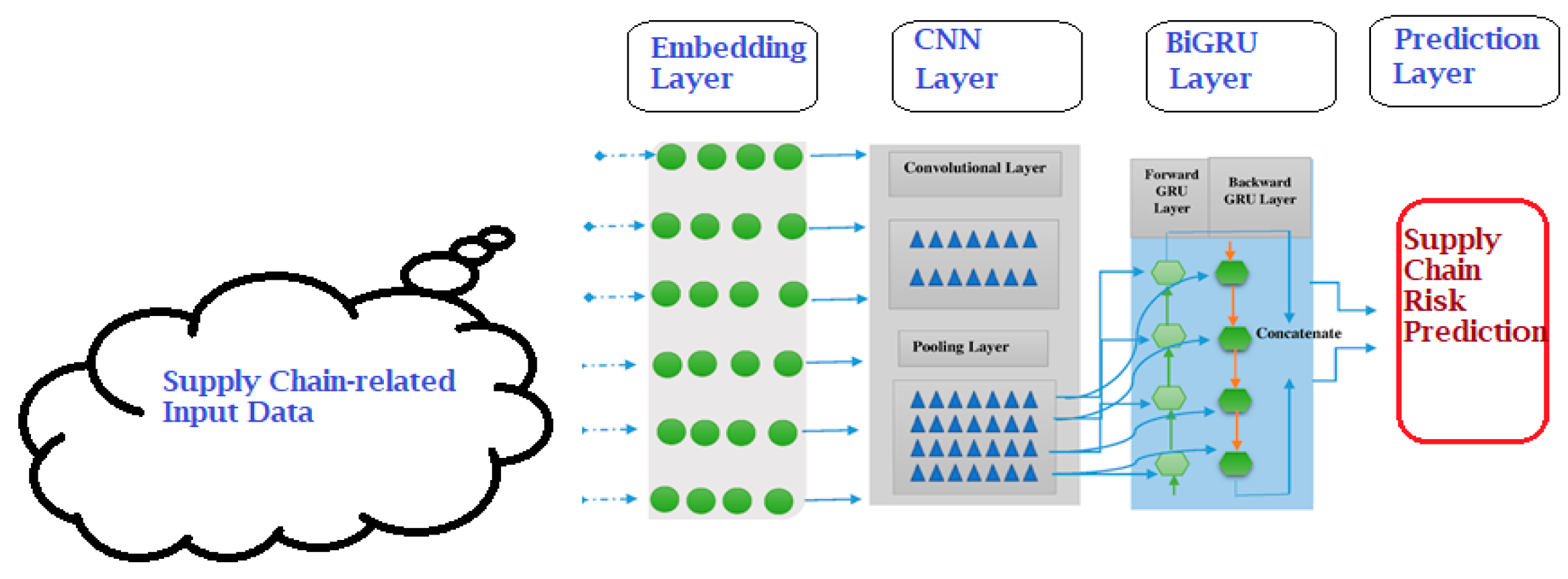
The proposed model employs a sigmoid activation function to categorize the BiGRU layer’s output into two categories: whether products may be shipped from a source location to a destination (yes or no). The proposed system accepts input data from the BiGRU and categorizes it into binary classes at the output layer using the sigmoid activation function (see Figure 2).

Figure 2. Detailed view of the proposed system.

3.8. Applied Example

The proposed composite model is made up of four separate layers. The first layer is the embedding layer, which assigns each element a low-dimensional vector. The CNN model is used in the feature extraction layer. The GRU layer, which explores the contextual portrayal of a data stream, makes up the third layer. The fourth layer in the neural network architecture, the output layer, is in charge of producing the results of shipment classification.

3.8.1. Embedding Layer

In this study, the information-integrating vectors were generated with the use of a Keras embedding layer. Within the embedding layer, the following steps were taken to create a two-dimensional embedding structure, also known as a feature matrix: $W\in {\mathcal{R}}^{t\times n}$. The quantity describing the size of the input data is represented by the symbol ‘t’, while the dimensionality of an element’s embedding is represented by the symbol ‘n’. Following the construction of an embedded matrix, it is moved to the next layer. Following that, the aforementioned matrix is sent to the CNN layer, which extracts the relevant features from the provided input data.

3.8.2. CNN Layer

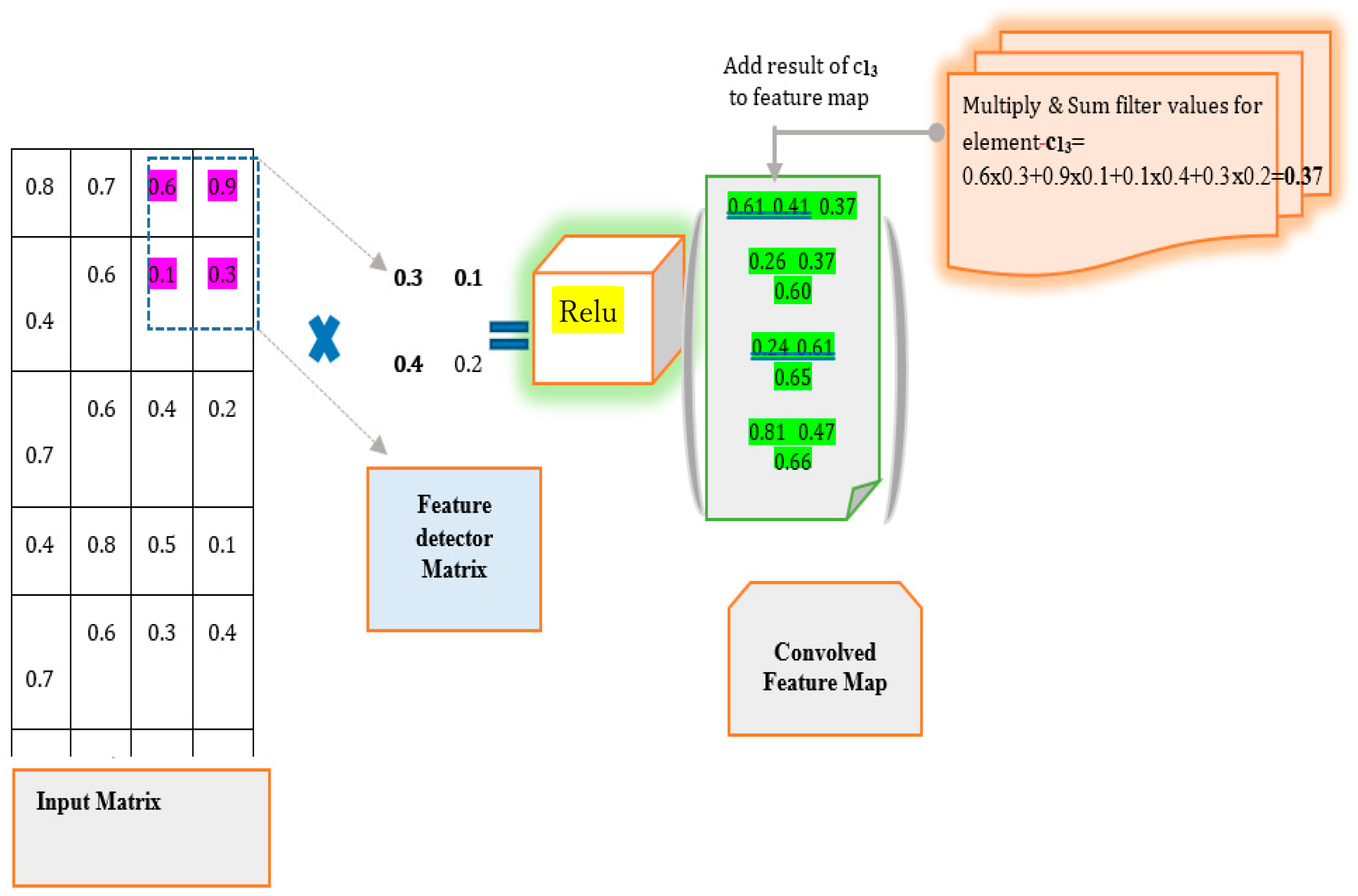
The CNN is made up of a single layer that is made up of two separate components, or modules. The following is a diagram of the CNN layer’s constituent elements: The core component of the CNN layer is the sliding of a feature recognition matrix over an input matrix to build a map of the feature matrix (see Figure 3). The feature recognition matrix has unique values that allow significant attributes in the input matrix to be identified [25].

Figure 3. Convolution operation.

The maxpooling procedure was used to improve the efficiency of the CNN layer by reducing the size of the convolved feature map [26]. The maxpooling operation is a pooling approach that produces a pooled feature map. The following steps are involved in the pooling layer’s execution. The procedure for obtaining a suitable window size is as follows: The suitable window size is first chosen. As a result, a stride of size 1 is chosen. Finally, the maximum values are chosen as the output. The resulting output is frequently referred to as a pooled feature map

3.8.3. BiGRU Layer

The current stage involves the computation of the forward ${GRU}^f$ and previous ${GRU}^b$ through the application of Equation (12). This results in the attainment of the representation $\stackrel{⃡}{GRU}$, which can be stated as outlined below:

$$\begin{array}{ccccc}\overleftrightarrow{GRU}& & GR{U}^f& & GR{U}^b\\ & & & & \\ 0.7& & 0.4& & 0.3\\ 0.3& =& 0.1& \oplus & 0.2\\ 0.6& & 0.5& & 0.1\\ 0.9& & 0.3& & 0.6\end{array}$$

3.8.4. Output Layer

This layer classifies shipments as (Yes/No) transportable from a source place to a destination. The total input during the first phase is calculated using the following formula (Equation (13)):

$${\mathrm{O}}_{in}=u1·w1+u2·w2+u3·w3\dots \dots uz·wz+b$$

(13)

We entered the following numbers in the formula above: as u$1 \mathrm{t}\mathrm{o} u4 (u1=0.7,u2=0.3,u3=0.6,u4=0.9),w1$$\mathrm{t}\mathrm{o} w4 (w1=0.1,w2=0.3,w3=0.4,w4=0.1) \mathrm{a}\mathrm{n}\mathrm{d} b=0.3.$

We have ${y\mathrm{O}}_{in}=0.7\times 0.1+0.3\times 0.3+0.6\times 0.4+0.9\times 0.1+\left(0.3\right)$=> ${\mathrm{O}}_{in}$=$0.79$.

After determining the total input, the second step uses the following function for sigmoid activation:

Making use of a sigmoid activation function.

The input is represented as y_in, whereas $y=f\left({\mathrm{O}}_{in}\right),$ indicates the output, and: $y=f\left({\mathrm{O}}_{in}\right),$ is the activation function.

$$\begin{gathered} => \mathrm{O}=\raisebox{1ex}{$1$}\!\left/ \!\raisebox{-1ex}{$1+e^{-{\mathrm{O}}_{in}}$}\right. \\ =\raisebox{1ex}{$1$}\!\left/ \!\raisebox{-1ex}{$1+e^{-0.79}$}\right. \\ \mathrm{O}=0.7 \\ f\left(x\right)=\left\{\begin{array}{c}1\left(pos\right),\hspace{1em}\mathrm{O}>0.5\\ 0\left(neg\right),\hspace{1em}otherwise\end{array}\right. \end{gathered}$$

Following the execution of the aforementioned computation, the value of y is equal to 0.7, which is more than 0.5. As a result, the shipment risk may be anticipated as follows: “Goods can be delivered from a source location to a destination = “yes””.

Table 4 provides a list of the mathematical symbols used in the various layers.

Table 4. Mathematical notation used in different layers.

Layer	Mathematical Symbol	Description
Embedding	$D$	Dataset
	$w$	Represent the words in a dataset
	$R$	Set of real numbers
	I	Input matrix
CNN	$\mathrm{M}$	Filter matrix
	$\mathrm{O}$	Output matrix
	$\mathrm{P}$	Pooled feature matrix
	I	Input matrix
	$\mathrm{R}$	Real number
	$b$	Bias term
	$f$	Activation function
	$\mathrm{H}$	Rectified feature map
BiGRU	$z$	Update gate
	$r$	Reset gate
	$x_t$	Input vector
	$s_t$	Cell state
	$W$	Input weight
	$U$	Output weight

The algorithmic steps of the suggested model are delineated in Algorithm 1.

Algorithm 1: Algorithm for predicting risks in supply chains using a CNN-GRU model

Step I: Import the dataset in the form of an xlsx file.              Step II: Split using scikit into train-test).                Step III: Develop the dictionary for associating integers with CICDDoS2019                Step V: procedure of BiGRU+CNN MODEL (NRtrain,Rtrain) #The deep learning model uses a layered method [E,B,C,M,S].              model = Sequential ()                #  Embedding Layer to map numbers to low-dimensional vectors model.add(Embedding(max_features,embed_dim,input_length = max_len))              #BiGRU Layer              model.add (Bidirectional (GRU (100))              #Convolutional Layer              model.add (Conv1D (filters=6, kernelsize=3, padding=’ same’,activation=’ relu’)              #Maxpooling Layer              model.add (MAxPooling1D (poolsize=2))                #Prediction of Supply chain Risks using Sigmoid Layer              model.add (Dense (2,activation=’ sigmoid’))                    #Fitting a model using train data              model.fit ()              #Compiler Function              model.compile () #Assess the performance of the model using the test dataset              Supply_chain_risk=model.evaluate ()     #The anticipated supply chain risk is being reported as either a positive                    or negative shipment outcome.                   return predicted supply_chain_risk                End Procedure

3.9. The Supply Chain Risk Prediction Model’s User Interface

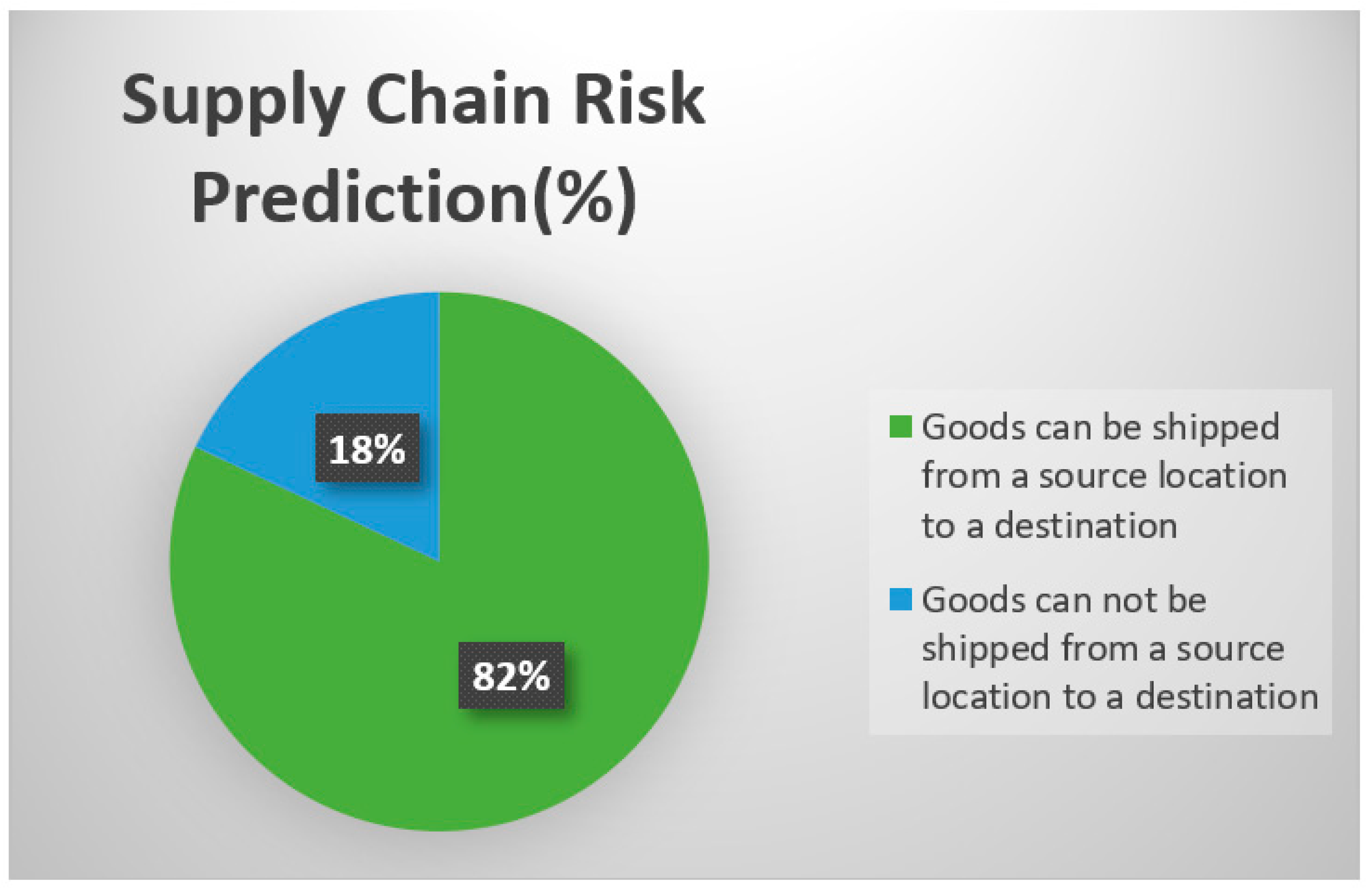
With a focus on usability, an online application was created to estimate SC risks based on benchmark data. The DL model was trained using the Keras toolkit and a Python-based Flask environment [23]. The model forecasts the likelihood of items being sent with a particular degree of certainty, resulting in either a positive or negative outcome for the goods shipment. Figure 4 depicts the SC risk for the supplied dataset when the goods_can_be_shipped variable is set to “yes”.

Figure 4. Supply chain risk prediction’s output.

4. Experimental Results

The following section shows the results of using the suggested deep learning (DL) technique on a benchmark dataset. The tests were carried out on a laptop equipped with a 12th Gen Intel^® Core™ i7-1250U processor running at Intel^® Iris^® Xe Graphics, 512 GB SSD, and a 16 GB LPDDR5. The Python programming language with Anaconda framework was used to create deep learning models and classifiers. The dataset contains 4,547,661 shipments in total. A subset of 2,048,577 shipments was chosen to evaluate the effectiveness of the suggested models in forecasting and predicting tasks. Based on the information provided with each shipment, the primary goal is to decide whether or not a shipment will be exported. This forecast is extremely useful in dangerous situations such as floods, earthquakes, and the recent COVID-19 pandemic. To execute the experiments, the selected shipments were separated into three groups: 50% for training, 25% for validation, and 25% for testing. This split resulted in 1,048,576 shipments in the training set and 500,001 shipments in each of the validation and test sets. The experiment included testing the performance of various DL models, including CNN, BiGRU, and others. The performance evaluation took into account several model training options, statistical performance metrics, and confusion metrices. Finally, various machine learning and DL classifiers were employed to validate the proposed DL model. This validation approach sought to evaluate the proposed model’s efficacy and generalizability by comparing its performance to that of other established classifiers. In summary, the section presented gives a description of the experimental setup, model creation, performance evaluation measures, and verification of the proposed DL model using several classifiers.

A variety of trials were carried out to answer the research questions provided in Section 1, and the results are presented in this section of the paper.

4.1. Addressing the Research Questions

4.1.1. Addressing the First Research Question

To address RQ.1: “When given a benchmark data set, how accurately does the CNN + BiGRU composite DL model predict supply chain risks in the logistics sector?”, the study used various CNN + BiGRU models with parameter settings to classify shipments based on supply chain risks. The classification was based on two distinct labels: whether items may be shipped from a source place to a destination (yes) or whether they cannot (no). The CNN + BiGRU models were built by modifying the parameters associated with each layer. To produce the best CNN + BiGRU simulation on the standard dataset, we used a parameter-tweaking approach inspired by the methods used in [3]. Table 5 displays a set of parameters that were optimized during model training.

Table 5. CNN + BIGRU configuration parameters.

CNN Model:	BIGRU Model:	Other Parameters:
Convolutional layer (filter size = 3 and padding = same) Pooling layer (pool size = 2)	GRU layer (units = 100)	Dense Layer (optimizer: adam, activation: sigmoid) Embedding Layer ( max _features: 2000, embed_dim: 128)

Table 6 shows the configuration of ten CNN + BiGRU models, each with a parameter combination of filter number, filter size, pool size, and BiGRU layer unit. The filter parameter values remain constant at 2 to 20, whereas the filter size, pool size, and BiGRU units do not change (see Table 7). This is due to the fact that changing these parameters has no noticeable effect on the model’s efficiency.

Table 6. CNN + BIGRU parameters for the model setup.

Model	Parameters
CNN + BIGRU1	filter count (2)
CNN + BIGRU2	filter count (4)
CNN + BIGRU3	filter count (6)
CNN + BIGRU4	filter count (8)
CNN + BIGRU5	filter count (10)
CNN + BIGRU6	filter count (12)
CNN + BIGRU7	filter count (14)
CNN + BIGRU8	filter count (16)
CNN + BIGRU9	filter count (18)
CNN + BIGRU10	filter count (20)

Table 7. Common parameters for each model.

Model	Common Parameters
CNN + BIGRU1 to CNN + BIGRU10	filter size (3), pool size (2), units (100)

Table 7 shows that filter size, pool size, and units are common for all models.

Performance Evaluation Metrices

Accuracy: The model’s accuracy is a measure of how well it predicts or classifies instances. It computes the proportion of correctly classified examples to the total number of occurrences in the dataset (see Equation (14)). The accuracy of the model offers an overall evaluation of its correctness.

$$\mathrm{A}\mathrm{c}\mathrm{c}\mathrm{u}\mathrm{r}\mathrm{c}\mathrm{a}\mathrm{y}=\frac{\mathrm{T}\mathrm{P}+\mathrm{T}\mathrm{N}}{\mathrm{T}\mathrm{P}+\mathrm{F}\mathrm{P}+\mathrm{T}\mathrm{N}+\mathrm{F}\mathrm{N}}$$

(14)

Precision: Precision, on the other hand, is a measure of how reliable or precise the model’s positive predictions are. It focuses on the instances that the model predicted as positive and calculates the ratio of correctly predicted positive instances to the total number of instances predicted as positive (see Equation (15)).

$$\mathrm{P}\mathrm{r}\mathrm{e}\mathrm{c}\mathrm{i}\mathrm{s}\mathrm{i}\mathrm{o}\mathrm{n}=\frac{\mathrm{T}\mathrm{P}}{\mathrm{T}\mathrm{P}+\mathrm{F}\mathrm{P}}$$

(15)

Recall: The ratio of true positive predictions to the total number of actual positive cases in the data is described as recall, also known as sensitivity or true positive rate. To put it another way, it quantifies the fraction of positive events properly detected by the model (see Equation (16)).

$$\mathrm{R}\mathrm{e}\mathrm{c}\mathrm{a}\mathrm{l}\mathrm{l}=\frac{\mathrm{T}\mathrm{P}}{\mathrm{T}\mathrm{P}+\mathrm{F}\mathrm{N}}$$

(16)

F1-score: The F1-score is defined as the harmonic mean of precision and recall and is calculated using the following formula (Equation (17)):

$$\text{F1-score}=2 \times \frac{\mathrm{P}\mathrm{r}\mathrm{e}\mathrm{c}\mathrm{i}\mathrm{s}\mathrm{i}\mathrm{o}\mathrm{n}\times \mathrm{r}\mathrm{e}\mathrm{c}\mathrm{a}\mathrm{l}\mathrm{l}}{\mathrm{P}\mathrm{r}\mathrm{e}\mathrm{c}\mathrm{i}\mathrm{s}\mathrm{i}\mathrm{o}\mathrm{n}+\mathrm{r}\mathrm{e}\mathrm{c}\mathrm{a}\mathrm{l}\mathrm{l}}$$

(17)

where TN stands for true negative, FN for false negative, FP for false positive, and TP for true positive.

Table 8 shows the results of several performance indicators, such as F1-score, precision, and recall. The CNN + BiGRU(3) model achieves a maximum accuracy of 94%, with the results showing a filter number of 6, a unit size of 100, and an F1-score, recall, and precision values of 94%. The CNN + BiGRU(1) model achieved 93% accuracy using a filter_size of 2 and a unit_size of 100. The CNN + BiGRU(2) model achieved 91% accuracy with a filter_size set to 2 and the unit_size set to 100. Several investigations have revealed that as the number of filters in the model increases the model’s performance gradually degrades.

Table 8. CNN + BIGRU model accuracy, recall, and F1-scores.

Model	Precision (%)	Recall (%)	F1-Score (%)
CNN + BIGRU1	93	93	93
CNN + BIGRU2	91	91	91
CNN + BIGRU3	94	94	94
CNN + BIGRU4	91	91	91
CNN + BIGRU5	92	92	92
CNN + BIGRU6	91	91	91
CNN + BIGRU7	93	93	93
CNN + BIGRU8	91	91	91
CNN + BIGRU9	91	91	91
CNN + BIGRU10	93	93	93

Table 9 shows the accuracy metric in connection with the loss score and BiGRU unit size. Accuracy and loss are two often-used measures in deep learning models to evaluate a model’s performance during training and testing. While accuracy is a simple measure of performance, the loss value provides more specific information about how effectively the model is learning. During the training phase, the loss value is often used to alter the model’s parameters. The model learns to generate increasingly accurate predictions by minimizing the loss score [27].

Table 9. Accuracy and loss values for all models (size of the unit = 100).

Model	Accuracy (%)	Loss Score (%)
CNN + BIGRU1	93	0.43
CNN + BIGRU2	91	0.27
CNN + BIGRU3	94	0.32
CNN + BIGRU4	91	0.37
CNN + BIGRU5	92	0.40
CNN + BIGRU6	91	0.41
CNN + BIGRU7	94	0.42
CNN + BIGRU8	91	0.43
CNN + BIGRU9	91	0.44
CNN + BIGRU10	93	0.45

4.1.2. Addressing the Second Research Question

Multiple experiments were conducted to compare the efficacy of the proposed methodology to established alternative ML methodologies. Table 10 shows the results of the experimental investigation of the proposed model and ML approaches.

Table 10. Comparison of the proposed model with ML techniques.

Model	Acc. (%)	Prec. (%)	Rec. (%)	F1-Score (%)
Support vector machine (ML)	86	88	86	86
Logistic regression (ML)	80	84	81	80
Random forest (ML)	82	83	82	82
Decision tree (ML)	87	87	87	87
ML [13]	83.21	83.21	83.21	83.21
CNN + BIGRU (DL)	94	94	94	94

ML: In this study, we used standard feature representation approaches to test the performance of various ML classifiers. According to the experimental results, the decision tree (DT) model performed the best, reaching an accuracy rate of 87%. The logistic regression (LR) model, on the other hand, had the lowest level of accuracy, with an accuracy rate of 80%.

Proposed model (CNN + BiGRU): Furthermore, we ran an experiment in which the proposed DL-based method, CNN + BiGRU, was utilized to classify logistics risk into one of two possible categories (shippable or not) based on data predictions. Table 10 demonstrates that the CNN + BiGRU model, which used the sophisticated embedding method, outperformed the other ML models.

In comparison to the proposed approach, the table below summarizes a number of the reasons why ML algorithms perform poorly.

Proposed model vs. SVM: In the current study, we employed a classifier trained with SVM, and it achieved a classification accuracy of 85.01%, implying that the SVM classifier we used was only 8% as successful as the suggested CNN + BiGRU model. The SVM classifier’s poor performance is due to its incompatibility with large datasets, as well as the time necessary to train on such data. Another issue with the procedure is overfitting [7].

Proposed model vs. LR: In the subsequent trial, the LR method was applied. According to Table 10, the LR algorithm only achieved a 79.85% success rate, 0.83 precision, 0.80 recall, and a 0.79 F1-score. The LR algorithm fared poorly compared to the suggested technique [7]. This is due to the LR algorithm’s inability to adequately record all of the complex interactions in the dataset.

Proposed model vs. RF: The objective of the investigation was to compare the effectiveness of the proposed framework to a random forest (RF) classifier constructed using machine learning. The RF classifier performed inefficiently, achieving an accuracy of 81.34%, resulting in an 11.66% decrease in efficiency compared to the suggested model. The RF technique’s fundamental limitation is its vulnerability to overfitting, which also requires a large amount of time for hyperparameter optimization [27], resulting in inferior efficiency.

Proposed model vs. MNB: Table 10 shows the results of using the multinomial naive Bayes algorithm. The results demonstrate that the MNB approach performed the worst among the other ML methods and the proposed method, with an accuracy of 78.36%. The MNB algorithm’s main disadvantage is a lack of data. Furthermore, it is unable to comprehend how various traits interact with one another. Furthermore, there is a chance that the procedure will lose accuracy [10].

Proposed model vs. DT: In the following experiment, the DT technique was used to compare its efficacy with the suggested CNN + BiGRU structure. The DT technique had an accuracy rating of 86.57%, showing a 6.43% drop in efficacy. The DT algorithm’s inferior efficiency might be linked to its intrinsic instability, in which even tiny changes in the input data can result in major changes to the decision tree’s framework. Furthermore, the training process for the model requires additional time. In comparison to alternative ML approaches, this algorithm is more sophisticated [7].

Proposed model vs. KNN: The authors conducted a comparative analysis in this study between their proposed technique and the prediction of SC risks in the logistics sector. One of the key limitations of the K-nearest neighbour (KNN) algorithm is its limited efficacy when applied to large datasets. Furthermore, the technique is vulnerable to the influence of outliers in the dataset. When used on imbalanced datasets, the K-nearest neighbours (KNN) algorithm exhibits inefficiency [10].

According to the results of the aforementioned studies, the CNN + BiGRU model outperformed ML classifiers in the classification of SC hazards. The benchmark dataset was used to investigate the performance of several baseline ML classifiers.

4.1.3. Addressing the Third Research Question

A comparison analysis was undertaken in response to RQ3, which pertains to the assessment of the usefulness of the proposed methodology in anticipating SC risks in the logistics industry relative to benchmark studies and other DL methodologies. Using a reference dataset, the efficacy of the proposed technique was compared to several types of deep learning. Table 11 shows the results of the experiment that was carried out.

Table 11. Performance evaluation of alternative deep learning approaches compared to the suggested approach.

Model	Acc. (%)	Pre. (%)	Rec. (%)	F1-Score (%)
RNN	87	87	87	87
BIGRU	91	91	91	91
CNN	90	90	90	90
GRU	90	90	90	90
CNN + BIGRU	94	94	94	94

RNN vs. proposed model (CNN + BiGRU): A DL approach, namely RNN, was used to compare its efficacy to the suggested CNN + BiGRU approach. Table 11 shows that the simple RNN outperformed our suggested technique in terms of precision, recall, and F1-score, with 87 percent precision, recall, and F1-score. This is due to the difficulties that the RNN has with gradient vanishing and bursting. Furthermore, it has been observed that the RNN has limitations in its ability to process and analyse long sequences [10]. As a result, it produced inferior results.

DL variants vs. proposed model (CNN + BiGRU): This section compares the suggested strategy (CNN + BiGRU) against several DL techniques employing advanced feature representation.

CNN vs. proposed model (CNN + BiGRU): The objective of this experiment was to compare the efficacy of the proposed CNN + BiGRU model to the CNN model using an experiment. The experimental results show that the CNN performed suboptimally, with accuracy, precision, recall, and an F1-score of 90%. In comparison, the CNN + BiGRU model performed better, with higher accuracy, precision, and recall, and an F1-score of 94%. The lower performance of the CNN in comparison to our proposed method can be attributed to the CNN’s failure to preserve the sequential organization of textual data, resulting in suboptimal classification results [24].

GRU vs. proposed model (CNN + BiGRU): The current study evaluated the efficacy of the proposed strategy (CNN + BiGRU) in contrast to the one-layer version of the GRU approach. In comparison to the suggested technique, the trial results show that the GRU had suboptimal efficiency, with an accuracy of 89 percent, a precision of 89 percent, a recall of 89 percent, and an F1-score of 89 percent. This is due to the GRU’s failure to extract its most important pieces from the data, as mentioned in reference [10].

BiGRU vs. proposed model (CNN + BiGRU): Finally, the BiGRU model was used to assess its effectiveness in conjunction with the suggested CNN + BiGRU model. The results indicate that the bidirectional gated recurrent unit (BiGRU) performed poorly, with an accuracy rate of 91%, a precision rate of 91%, a recall rate of 91%, and an F1-Score of 91%. These results are less precise than the proposed CNN technique combined with BiGRU. The fundamental limitation of the BiGRU model in terms of the proposed methodology is its insufficient efficacy in feature extraction, as indicated in reference [24].

The CNN + BiGRU model outperformed previous DL-based models, obtaining an excellent accuracy rate of 94 percent. The BiGRU model achieved 90% accuracy, whereas the GRU and CNN algorithms achieved 90% accuracy. The simple RNN model achieved an accuracy of 87 percent.

4.2. Comparison with Baselines

To evaluate the effectiveness of the proposed technique under consideration, it is compared to the baseline technique.

ML technique: In the logistics sector, [13] introduced a supervised ML approach to forecast SC risks. Nonetheless, the system employed a conventional feature representation approach, thereby warranting further exploration of deep neural networks that incorporate sophisticated embedding schemes to enhance efficacy.

DL technique: Bassiouni et al. [3] applied a TCN model to predict supply chain risks during COVID-19 restrictions. Their technique achieved promising results; however, lack of capturing context information resulted in performance degradation.

Deep-supply-chains (proposed model): This study employs a hybrid deep neural network architecture, specifically the combination of CNN and bidirectional gated recurrent unit (BIGRU), to forecast potential SC risks within the logistics industry. According to Table 12, the performance of the suggested structure surpasses that of comparable methods developed for predicting SC risk (see Table 12). Additionally, we compared the proposed system with three more studies, i.e., Hu et al. [1], Dong et al. [5], and Liu et al. [10]. The results presented in Table 12 show that our proposed technique surpasses the mentioned works.

Table 12. Comparison with baselines (A: accuracy, P: precision, R: recall, F: F1-Score).

Technique	A (%)	P (%)	R (%)	F (%)
Supply chain prediction with DL [3]	85.71	86.52	85.11	87.32
Supply chain prediction with ML [13]	83.21	84.62	84.09	84.56
Supply chain prediction with DL (proposed CNN + BIGRU)	94	94	94	94
Hu et al. [1]	86.88	87.71	88.31	87.97
Dong et al. [5]	81	80.52	80.0	81.0
Liu et al. [10]	84.22	87.17	86.71	88.21

4.3. Summary of the Results and Discussion

This paper presents a novel study that employs an efficient deep learning approach to assess the exportability of goods during floods, earthquakes, and the recent COVID-19 epidemic. Given the scarcity of case studies examining the application of deep learning techniques in supply chain management, the primary goal is to provide insights into the creation and implementation of deep learning methodology for analysing supply chain data.

4.3.1. Analysis of the Results

Based on the data reported in the preceding tables, the RNN, CNN, GRU, and BiGRU techniques performed satisfactorily. Among them, the BiGRU strategy outperformed the RNN and GRU approaches in terms of accuracy, but with a slight difference in decimals. This shows that combining CNN and BiGRU layers considerably improves overall performance. The classification step was the final stage of the study, in which classifiers were used to classify the test data. To evaluate the classifier’s performance and obtain the final accuracy result, various performance measurements were used. The performance evaluation is shown in the results tables, which show that the RT, RF, KNN, and SVM classifiers performed the best in the classification stage. When compared to ML classifiers that did not use DL techniques, the DL models improved prediction accuracy by 13.526%. These findings highlight the robustness and strength of DL models in this situation. They also confirm the effectiveness of DL models’ autonomous feature extraction capabilities in assisting ML classifiers in producing accurate forecasting results. When the accuracy of ML techniques is compared, it becomes apparent that they misclassified a large number of shipments, regardless of their export status. In contrast, the use of DL models such as CNN, RNN, LSTM, BiLSTM, and BiGRU increased classification performance for shipments that were not exported. These DL models outperformed the ML techniques in terms of accuracy. Notably, the proposed CNN + BiGRU model, which combines CNN and BiGRU, outperformed both classes of shipments, even when dealing with fewer shipments in one of the two classes. The CNN + BiGRU method combines two distinct DL architectures: the CNN and the bidirectional gated recurrent unit (BiGRU). Because it incorporates both CNN and bidirectional gated recurrent units (BiGRU), the proposed approach outperforms previous DL algorithms. The CNN model excels at preserving local dependencies while extracting features, whereas the bidirectional gated recurrent unit (BiGRU) model can preserve information over long periods of time in both the forward (future) and backward (past) directions. As a result, the study indicates that the CNN + BiGRU model displayed significant prediction skills in the field of SC risk by utilizing the advanced depiction of term embedding. This was accomplished by efficiently combining the strengths of the CNN and BiGRU models.

4.3.2. Summary of Theoretical and Practical Contributions

The proposed intelligent supply chain risk prediction system can contribute both theoretically and practically. Here are some possible contributions:

Contributions to Theory: (i) Knowledge advancement: The proposed intelligent supply chain risk prediction system advances theoretical understanding of supply chain risk management by offering novel methodologies, models, and algorithms. It may improve our understanding of how various elements and variables influence supply chain risk. (ii) Framework creation: The proposed system contributes to the creation of theoretical frameworks that incorporate numerous risk elements into a unified risk prediction model, which can assist scholars and practitioners in better understanding the complex dynamics of supply chain risk, such as demand variability, supplier reliability, geopolitical events, and natural disasters. (iii) Methodological advances: Intelligent prediction systems often analyse and predict supply chain risks using cutting-edge AI-based deep learning techniques. This methodological advancement contributes to a theoretical understanding of how these techniques can be effectively used in supply chain risk management.

Practical Contributions: (i) Improved risk management: The proposed intelligent supply chain risk prediction system adds real value by allowing organizations to proactively identify and analyse potential risks in their supply chain. This assists managers in developing effective risk mitigation strategies and contingency plans that reduce the impact of disruptions and improve supply chain resilience. (ii) Improved decision-making: By delivering accurate and timely risk projections, the suggested technologies aid in supply chain management decision-making. Managers may make informed decisions on sourcing, inventory management, transportation, and other operational issues by taking into account the anticipated risks and their potential impact. (iii) Cost reductions can be gained by anticipating and minimizing supply chain risks. Organizations can prevent downtime, inventory losses, and costly emergency measures by avoiding or minimizing disruptions. This improves cost efficiency and overall financial performance. (iv) Competitive advantage: Implementing the proposed intelligent supply chain risk prediction system can provide organizations with a competitive advantage by allowing them to manage risks proactively, ensure business continuity, and provide products/services to consumers in a reliable manner. It increases client happiness and promotes the organization’s market reputation.

Overall, the proposed intelligent supply chain risk prediction system advances knowledge, improves risk management practises, enables better decision-making, reduces costs, and offers a competitive advantage in the dynamic and unpredictable world of supply chain management.

4.3.3. Generalizability of Experimental Results

The following aspects were studied and extensively examined in order to assess the generalizability of the experimental outcomes of the proposed intelligent supply chain risk prediction system. Here is a thorough breakdown of the factors we considered:

Data collection: The quality and representativeness of the data used for training and testing determine the generalizability of the system’s results. By incorporating a wide range of benchmark data, one can increase the possibility of capturing various risk patterns and contextual elements, thereby improving generalizability because the information gathered covers a wide range of sectors, supply chain architectures, geographical locations, and time periods.

Model design and algorithm selection: It is critical for generalizability to select proper modelling approaches and algorithms. From the literature review and the experiments that we conducted, it is ensured that the proposed model architecture and algorithm are appropriate for capturing the complexity and dynamism of supply chain risk.

Performance assessment: The intelligent system’s performance is assessed using robust assessment metrics, to evaluate the system’s predictive skills across multiple subsets, dividing the data into training, validation, and testing sets and undergoing cross-validation. To fully assess the system’s performance, we considered parameters such as accuracy, precision, recall, and F1-score.

4.3.4. Research Implications and Insights

The proposed work on an intelligent supply chain risk prediction system may have far-reaching implications for both academics and the industry. Here are some potential implications and insights:

Improved risk management: Our research helps to improve supply chain risk management practices. Organizations can proactively detect and assess potential risks by establishing an intelligent system for forecasting supply chain risks. This helps them put effective risk mitigation procedures in place, lowering the frequency and severity of disruptions.

Improved supply chain resilience: The conclusions of this study might assist organizations in increasing their supply chain resilience. Organizations can improve their ability to absorb and recover from disruptions by effectively identifying risks. Diversifying supplier networks, developing backup plans, and implementing contingency plans are all part of ensuring business continuity.

Cost savings: Accurate risk prediction can result in cost savings in supply chain operations. Organizations may avoid costly disruptions, minimize downtime, reduce inventory losses, and optimize logistics and transportation by detecting and reducing potential risks in advance. This increases cost efficiency and financial success overall.

Strategic decision-making: This research gives insights for strategic supply chain management decision-making. By taking into account expected risks and their potential impact, the intelligent system can aid decision-makers in evaluating various methods such as supplier selection, inventory management, and distribution network design. As a result, decision-making becomes more informed and effective.

Competitive advantage: A competitive advantage can be gained by implementing an intelligent supply chain risk prediction system. Organizations that can handle risks effectively have better resilience, dependability, and responsiveness. This improves their market reputation and helps attract clients and partners who seek a secure and resilient supply chain.

Technological progress: This work helps to progress technology in the field of supply chain risk management. We are pushing the frontiers of what is feasible in terms of risk prediction and mitigation by inventing and implementing intelligent systems. This brings up new opportunities for innovation and research in the fields of supply chain management and artificial intelligence.

Expansion of knowledge: This research adds to the body of knowledge in the field of supply chain risk management. One can improve the grasp of the underlying causes and dynamics of supply chain hazards by performing thorough research. This knowledge can be shared with academics and practitioners in the industry, supporting future studies and practical applications.

Overall, the implications and insights of the proposed intelligent supply chain risk prediction system include better risk management, increased supply chain resilience, cost savings, strategic decision-making, competitive advantages, technological advancement, and knowledge expansion in the field of supply chain management.

4.4. Complexity Analysis

Time complexity: The CNN + BiGRU model for binary classification in intelligent supply chain risk prediction has a time complexity that is determined by the length of the input sequence, the number of hidden entities in the GRU layers, the number of layers in the BiGRU architecture, and the amount of the input data. The suggested CNN + BiGRU model’s time complexity can be estimated as O(T × (N × M^2 × P + C × K^2 × H × W)), where T is the length of the input sequence, N is the number of hidden units in each GRU layer, M is the number of layers in the BiGRU model, P is the total number of parameters in the model, C is the number of channels in the input data, and K^2 × H × W is the number of operations performed by the CNN layer. The proposed CNN + BiGRU model required 588 min and 45 s to train.

Computational complexity: The computational complexity of a CNN + BiGRU model for binary classification in intelligent supply chain risk prediction is affected by a variety of factors, including the length of the input sequence, the number of hidden units in the GRU layers, the number of layers in the BiGRU architecture, the number of parameters in the model, and the size of the input data. The CNN + BiGRU model’s total complexity can be approximated as O(T × N × M^2 × P + C × K^2 × H × W), where T is the length of the input sequence and N is the number of input elements. The total number of hidden units is 1s in each GRU layer. The number M denotes the number of layers in the BiGRU model. The total number of parameters in the model is represented by P. C denotes the number of input data channels. The number of operations executed by the CNN layer is represented as K^2 × H × W. During the forward pass, the CNN component conducts operations on the input data such as convolutions and pooling, resulting in a complexity of about O(C × K^2 × H × W). The following BiGRU component processes the processed features, resulting in a complexity of about O(T × N × M^2 × P).

5. Conclusions and Future Work

This research focuses on the problem of predicting SC risk in the logistics business using a DL technique, specifically the BiGRU and CNN models. The suggested approach includes (i) data collection, (ii) a study of the proposed model, (iii) a description of the proposed model’s architecture, and (iv) a plan for implementing that structure.

The proposed BiGRU + CNN architecture is built on the combination of a bidirectional gated recurrent unit (BiGRU) with a convolutional neural network. By utilizing both forward and backward GRU, the BiGRU model leverages contextual data in a bidirectional manner. The CNN model, on the other hand, appropriately captures salient features. The study compares the effectiveness of the BiGRU + CNN model to that of many other DL models across multiple corpora. The results show that the BiGRU + CNN model outperformed the baseline models, with an accuracy of 93 percent, a precision of 93 percent, a recall of 93 percent, and an F1-score of 93 percent. The results obtained have the potential to help business owners make educated judgements before exporting their products. These measurements are based on probabilistic calculations and serve as a platform for practitioners to make more accurate forecasts about whether a shipment will be exported while accounting for uncertainties provided by events such as earthquakes, floods, and the COVID-19 pandemic. The digital revolution, notably Industry 4.0 and 5.0, has enabled industries to aggregate all of their supply chain data onto a uniform platform. Previously, it was widely assumed that enterprises needed a large amount of data and a strong data management plan in place before implementing recommended deep learning (DL) approaches. However, if a corporation has proper data management capabilities and a platform for accessing historical data, using these DL approaches should be rather simple. It should be emphasized that DL models rely substantially on data and software, hence adequate parallel computer resources are required to build such models.

Limitations: The proposed model has some drawbacks that should be mentioned. (i) The current study is primarily concerned with the binary categorization of SC risk. (ii) The dataset used in this study is unbalanced. (iii) The method used in this study did not require the use of a pre-trained CNN model but rather depended on the content-embedding technique.

Future Directions: (i) Rather than relying exclusively on binary predictions, the logistics industry can benefit from a more nuanced approach to identifying SC risks. Furthermore, the efficacy of the proposed method can be improved by using a balanced data set. (ii) Word2Vec, Glove, Fasttext, and other already-trained content-embedding methods can be integrated. (iii) Additional approaches and combinations of DL techniques can be explored for more reliable outcomes. (iv) Further research can be conducted on sophisticated iterations of the attention mechanism and BiGRU. (v) In the future, the amount and quality of the database used to train a neural network will be increased to provide a more thorough representation of the data’s underlying patterns and relationships. It allows for the collection of a broader range of events and variations, resulting in a more robust and accurate model. With more diverse instances, the neural network can learn to generalize more effectively and generate more accurate predictions on previously unseen data. (vi) External validation: Use external datasets or real-world case studies to validate the system’s predicted performance that were not included in the initial training and testing. This aids in determining if the algorithm can generalize its predictions to new and previously unseen data. When a system consistently performs well across numerous independent datasets or real-world settings, its generalizability improves. (vii) Conduct sensitivity analysis to analyse the system’s performance under various situations and input variations. Prove the system’s robustness by introducing various sorts of perturbations, such as changes in data quality, missing numbers, or risk-factor alterations. Examine how the system reacts to these changes and whether its predictions remain accurate and dependable.

References

1. Hu, H.; Xu, J.; Liu, M.; Lim, M.K. Vaccine supply chain management: An intelligent system utilizing blockchain, IoT and machine learning. J. Bus. Res. 2023, 156, 113480. [Google Scholar] [CrossRef]
2. Karumanchi, M.D.; Sheeba, J.I.; Devaneyan, S.P. Blockchain Enabled Supply Chain using Machine Learning for Secure Cargo Tracking. Int. J. Intell. Syst. Appl. Eng. 2022, 10, 434–442. [Google Scholar]
3. Bassiouni, M.M.; Chakrabortty, R.K.; Hussain, O.K.; Rahman, H.F. Advanced deep learning approaches to predict supply chain risks under COVID-19 restrictions. Expert Syst. Appl. 2023, 211, 118604. [Google Scholar] [CrossRef]
4. Singh, S.; Kumar, R.; Panchal, R.; Tiwari, M.K. Impact of COVID-19 on logistics systems and disruptions in food supply chain. Int. J. Prod. Res. 2021, 59, 1993–2008. [Google Scholar] [CrossRef]
5. Dong, Z.; Liang, W.; Liang, Y.; Gao, W.; Lu, Y. Blockchained supply chain management based on IoT tracking and machine learning. EURASIP J. Wirel. Commun. Netw. 2022, 2022, 127. [Google Scholar] [CrossRef] [PubMed]
6. Vo, N.N.; He, X.; Liu, S.; Xu, G. Deep learning for decision making and the optimization of socially responsible investments and portfolio. Decis. Support Syst. 2019, 124, 113097. [Google Scholar] [CrossRef]
7. Asghar, M.Z.; Ullah, I.; Shamshirband, S.; Khundi, F.M.; Habib, A. Fuzzy-based sentiment analysis system for analyzing student feedback and satisfaction. Comput. Mater. Contin. 2020, 62, 631–655. [Google Scholar]
8. Asghar, M.Z.; Habib, A.; Habib, A.; Khan, A.; Ali, R.; Khattak, A. Exploring deep neural networks for rumor detection. J. Ambient Intell. Humaniz. Comput. 2021, 12, 4315–4333. [Google Scholar] [CrossRef]
9. Cai, X.; Qian, Y.; Bai, Q.; Liu, W. Exploration on the financing risks of enterprise supply chain using back propagation neural network. J. Comput. Appl. Math. 2020, 367, 112457. [Google Scholar] [CrossRef]
10. Liu, Y.; Huang, L. Supply chain finance credit risk assessment using support vector machine–based ensemble improved with noise elimination. Int. J. Distrib. Sens. Netw. 2020, 16, 1550147720903631. [Google Scholar] [CrossRef]
11. Xu, C.; Ji, J.; Liu, P. The station-free sharing bike demand forecasting with a deep learning approach and large-scale datasets. Transp. Res. Part C 2018, 95, 47–60. [Google Scholar] [CrossRef]
12. Nikolopoulos, K.; Punia, S.; Schäfers, A.; Tsinopoulos, C.; Vasilakis, C. Forecasting and planning during a pandemic: COVID-19 growth rates, supply chain disruptions, and governmental decisions. Eur. J. Oper. Res. 2021, 290, 99–115. [Google Scholar] [CrossRef]
13. Pan, W.; Miao, L. Dynamics and risk assessment of a remanufacturing closed-loop supply chain system using the internet of things and neural network approach. J. Supercomput. 2023, 79, 3878–3901. [Google Scholar] [CrossRef]
14. Liu, C.; Ji, H.; Wei, J. Smart SC risk assessment in intelligent manufacturing. J. Comput. Inf. Syst. 2022, 62, 609–621. [Google Scholar]
15. Palmer, C.; Urwin, E.N.; Niknejad, A.; Petrovic, D.; Popplewell, K.; Young, R.I. An ontology supported risk assessment approach for the intelligent configuration of supply networks. J. Intell. Manuf. 2018, 29, 1005–1030. [Google Scholar] [CrossRef]
16. Lorenc, A.; Burinskiene, A. Improve the orders picking in e-commerce by using WMS data and BigData analysis. FME Trans. 2021, 49, 233–243. [Google Scholar] [CrossRef]
17. Keller, S. US Supply Chain Information for COVID19. Available online: https://www.kaggle.com/skeller/us-supply-chain-information-for-covid19 (accessed on 2 March 2023).
18. Baryannis, G.; Dani, S.; Antoniou, G. Predicting supply chain risks using machine learning: The trade-off between performance and interpretability. Future Gener. Comput. Syst. 2019, 101, 993–1004. [Google Scholar] [CrossRef]
19. Asghar, M.Z.; Albogamy, F.R.; Al-Rakhami, M.S.; Asghar, J.; Rahmat, M.K.; Alam, M.M.; Lajis, A.; Nasir, H.M. Facial Mask Detection Using Depthwise Separable Convolutional Neural Network Model During COVID-19 Pandemic. Front. Public Health 2022, 10, 855254. [Google Scholar] [CrossRef]
20. Liu, J.; Yang, Y.; Lv, S.; Wang, J. Attention-based BiGRU-CNN for Chinese question classification. J. Ambient Intell. Humaniz. Comput. 2019, 1–12. [Google Scholar] [CrossRef]
21. Agarwal, R. NLP Learning Series: Part 3—Attention, CNN and What Not for Text Classification. 2019. Available online: https://towardsdatascience.com/nlp-learning-series-part-3-attention-cnn-and-what-not-for-text-classification-4313930ed566 (accessed on 9 April 2023).
22. All Things Embedding. Available online: https://keras.io/layers/embeddings/ (accessed on 21 February 2023).
23. She, X.; Zhang, D. Text Classification Based on Hybrid CNN-LSTM Hybrid Model. In Proceedings of the 2018 11th International Symposium on Computational Intelligence and Design (ISCID), Hangzhou, China, 8–9 December 2018; Volume 2, pp. 185–189. [Google Scholar]
24. Rachel, D. How Computers See: Intro to Convolutional Neural Networks. 2019. Available online: https://glassboxmedicine.com/2019/05/05/how-computers-see-intro-to-convolutional-neural-networks/ (accessed on 25 March 2023).
25. Rabie, O.; Alghazzawi, D.; Asghar, J.; Saddozai, F.K.; Asghar, M.Z. A Decision Support System for Diagnosing Diabetes Using Deep Neural Network. Front. Public Health 2022, 10, 861062. [Google Scholar] [CrossRef]
26. Alghazzawi, D.; Bamasag, O.; Ullah, H.; Asghar, M.Z. Efficient detection of DDoS attacks using a hybrid deep learning model with improved feature selection. Appl. Sci. 2021, 11, 11634. [Google Scholar] [CrossRef]
27. Alghazzawi, D.; Bamasag, O.; Albeshri, A.; Sana, I.; Ullah, H.; Asghar, M.Z. Efficient prediction of court judgments using an LSTM+ CNN neural network model with an optimal feature set. Mathematics 2022, 10, 683. [Google Scholar] [CrossRef]
Disclaimer/Publisher’s Note: The statements, opinions and data contained in all publications are solely those of the individual author(s) and contributor(s) and not of MDPI and/or the editor(s). MDPI and/or the editor(s) disclaim responsibility for any injury to people or property resulting from any ideas, methods, instructions or products referred to in the content.
Article Metrics
Citations
Article Access Statistics
Multiple requests from the same IP address are counted as one view.